A Linear Time Delay Model for Studying Load
Balancing Instabilities in Parallel Computations
C. Abdallah
ECE Dept
University of NewMexico
Alburquerque NM 87131-1356
Nivedita Alluri, J. Douglas Birdwell, John Chiasson
Victor Chupryna and Zhong Tang
ECE Dept
University of Tennessee
Knoxville TN 37996, USA,
T. Wang
Chemical Engineering Dept
University of Tennessee
Knoxville TN 37996, USA,
June 28, 2002
Abstract
A linear time-delay system is used to model load balancing in a cluster of computer nodes used for parallel computations. The linear model is analyzed for stability in terms of the delays in the transfer of information between nodes and the gains in the load balancing algorithm. This model is compared with an experimental implementation of the algorithm on a parallel computer network.
1
Introduction
In this work, a linear time-delay system is used to model load balancing in a cluster of computer nodes used for parallel computations. The linear model is analyzed for stability in terms of the delays in the transfer of information between nodes and the gains in the load balancing algorithm. This model is compared with an experimental implementation of the algorithm on a parallel computer network. Preliminary results by the authors appear in [1], however, a change has been made to the linear model in [1] which represents betterÞdelity and also experimental results are reported here.
Parallel computer architectures utilize a set of computational elements (CE) to achieve performance that is not attainable on a single processor, or CE, com-puter. A common architecture is the cluster of otherwise independent computers communicating through a shared network. To make use of parallel computing resources, problems must be broken down into smaller units that can be solved individually by each CE while exchanging information with CEs solving other problems.
The Federal Bureau of Investigation (FBI) National DNA Indexing System (NDIS) and Combined DNA Indexing System (CODIS) software are candidates for parallelization. New methods developed by Wang et al [3][4][5][17][18] lead naturally to a parallel decomposition of the DNA database search problem while providing orders of magnitude improvements in performance over the current release of the CODIS software. The projected growth of the NDIS database and in the demand for searches of the database necessitates migration to a parallel computing platform.
Effective utilization of a parallel computer architecture requires the compu-tational load to be distributed more or less evenly over the available CEs. The qualiÞer “more or less” is used because the communications required to distrib-ute the load consume both computational resources and network bandwidth. A point of diminishing returns exists.
Distribution of computational load across available resources is referred to as theload balancingproblem in the literature. Various taxonomies of load balanc-ing algorithms exist. Direct methods examine the global distribution of compu-tational load and assign portions of the workload to resources before processing begins. Iterative methods examine the progress of the computation and the expected utilization of resources, and adjust the workload assignments period-ically as computation progresses. Assignment may be either deterministic, as with the dimension exchange/diffusion [8] and gradient methods, stochastic, or optimization based. A comparison of several deterministic methods is provided by Willeback-LeMain and Reeves [19].
To adequately model load balancing problems, several features of the par-allel computation environment should be captured (1) The workload awaiting processing at each CE; (2) the relative performances of the CEs; (3) the com-putational requirements of each workload component; (4) the delays and band-width constraints of CEs and network components involved in the exchange of workloads, and (5) the delays imposed by CEs and the network on the exchange of measurements. A queuing theory [15] approach is well-suited to the model-ing requirements and has been used in the literature by Spies [16] and others. However, whereas Spies assumes a homogeneous network of CEs and models the queues in detail, the present work generalizes queue length to an expected waiting time, normalizing to account for differences among CEs, and aggregates the behavior of each queue using a continuous state model. The present work fo-cuses upon the effects of delays in the exchange of information among CEs, and the constraints these effects impose on the design of a load balancing strategy.
Section 2 presents our approach to modeling the computer network and load balancing algorithms to incorporate the presence of delay in communicating
between nodes and transferring tasks. Section 3 contains an analysis of the stability properties of the linear models, while Section 4 presents simulations of the model. Section 5 presents experimental data from an actual implementation of a load balancing algorithm andÞnally, Section 6 is a summary and conclusion of the present work and a discussion of future work.
2
A Dynamic Model of Load Balancing
In this section, linear dynamic time-delay model is developed to model load balancing among a network of computers. To introduce the basic approach to load balancing, consider a computing network consisting ofncomputers (nodes) all of which can communicate with each other. At start up, the computers are assigned an equal number of tasks. However, when a node executes a particular task it can in turn generate more tasks so that very quickly the loads on various nodes become unequal. To balance the loads, each computer in the network sends its queue size qj(t)to all other computers in the network. A node i re-ceives this information from nodej delayed by aÞnite amount of timeτij, that is, it receives qj(t−τij). Each node i then uses this information to compute its local estimate1 of the average number of tasks in the queues of then com-puters in the network. In this work, the simple estimator³Pnj=1qj(t−τij)
´
/n
(τii = 0) which is based on the most recent observations is used. Node i then compares its queue size qi(t)with its estimate of the network average as ³
qi(t)−³Pnj=1qj(t−τij) ´
/n´and, if this is greater than zero, the node sends some of its tasks to the other nodes while if it is less than zero, no tasks are sent (see Figure 1). Further, the tasks sent by nodeiare received by node j with a delayhij. The controller (load balancing algorithm) decides how often and fast to do load balancing (transfer tasks among the nodes) and how many tasks are to be sent to each node.
1It is an estimate because at any time, each node only has the delayed value of the number
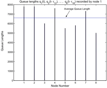
1 2 3 4 5 6 7 8 0 1000 2000 3000 4000 5000 6000 7000
8000 Queue lengths q1(t), q2(t-τ12), ... , q8(t-τ18) recorded by node 1
Node Number Q u eu e L en gt hs
Average Queue Length
Figure 1: Graphical description of load balancing. This bar graph shows the load for each computer vs. node of the network. The thin horizontal line is the average load as estimated by node1. Node1will transfer (part of) its load only if it is above its estimate of the average. Also, it will only transfer to nodes that it estimates are below the node average.
As just explained, each node controller (load balancing algorithm) has only delayed values of the queue lengths of the other nodes, and each transfer of data from one node to another is received only after a Þnite time delay. An important issue considered here is to study the effect of these delays on system performance. SpeciÞcally, the continuous time models developed here represent our effort to capture the effect of the delays in load balancing techniques and were developed so that system theoretic methods could be used to analyze them.
2.1
Dynamic Model
The basic mathematical model of a given computing node for load balancing is given by
dxi(t) dt =λi−µi+ui(t)− n X j=1 pij tpi tpj uj(t−hij) yi(t) =xi(t)− Pn j=1xj(t−τij) n (1) ui(t) =−Kiyi(t) pij >0, pjj = 0, n X i=1 pij = 1
where in this model we have
• nis the number of nodes.
• xi(t)is theexpected waiting time experienced by a task inserted into the queue of the ith node. With qi(t) the number of tasks in the ith node and tpi the average time needed to process a task on the i
th node, the expected (average) waiting time is then given byxi(t) =qi(t)tpi. Note that
xj/tpj =qjis the number of tasks in the node1queue. If these tasks were
transferred to nodei, then the waiting time transferred isqjtpi =xjtpi/tpj,
so that the fractiontpi/tpj converts waiting time on nodejto waiting time
on nodei.
• λi is the rate of generation of waiting time on theithnode caused by the addition of tasks (rate of increase inxi)
• µi is the rate of reduction in waiting time caused by the service of tasks at theithnode and is given byµ
i≡(1×tpi)/tpi = 1for alli.
• ui(t)is the rate of removal (transfer) of the tasks from node i at time t by the load balancing algorithm at nodei.
• pijuj(t)is the rate that nodejsends waiting time (tasks) to nodeiat time
twherepij>0,Pni=1pij = 1andpjj= 0. That is, the transfer from node
jof expected waiting time (tasks) Z t2
t1
uj(t)dtin the interval of time[t1, t2]
to the other nodes is carried out with theithnode being sent the fraction
pij tpi tpj
Z t2
t1
uj(t)dtwhere the fractiontpi/tpj converts the task from waiting
time on nodej to waiting time on node i. AsPni=1 µ pij Z t2 t1 uj(t)dt ¶ = Z t2 t1
uj(t)dt, this results in a removing all the waiting time Z t2
t1
uj(t)dt from nodej.
• The quantity−pijuj(t−hij)is the rate of increase (rate of transfer) of the expected waiting time (tasks) at timet from nodej by (to) nodeiwhere
hij (hii = 0)is the time delay for the task transfer from node jto nodei.
• The quantitiesτij (τii= 0)denote the time delay for communicating the expected waiting timexj from nodej to node i.
• The quantity xavgi = ³Pnj=1xj(t−τij) ´
/n is the estimate2 by the ith node of the average waiting time of the network and is referred to as the local average (local estimate of the average).
In this model, all rates are in units of therate of change of expected waiting time, ortime/time which is dimensionless). Thejthnode receives the fraction Z t2
t1
pjiui(t)dt of transferred waiting time Z t2
t1
ui(t)dt delayed by the timehij. As all nodes are taken to be identical, thepjifor each sending nodeiis speciÞed as constant and equal to
pji=p= 1/(n−1)forj6=i
pii= 0
where it is clear thatpij >0,Pni=1pij = 1.
A delay is experienced by transmitted tasks before they are received at the other node. The control law ui(t) = −Kiyi(t) states that if at the ith node,
ui(t) =−Kiyi(t)<0(yi(t)>0), then it sends data to the other nodes. How-ever, ifyi(t)<0, the controller (load balancing algorithm)ui(t) =−Kiyi(t)>0 so that the node isinstantaneouslytaking on waiting time (tasks) from the other nodes before those tasks are removed from the other nodes’ queues. As explained above, the actual network does not do this; if yi(t) < 0, then the local node does not initiate any transfer of tasks. That is, the actual network has a control law of the formui(t) =−Kisat(yi(t))where sat(y) =y ify>0and sat(y) = 0 ify < 0. However, in spite of this fact, the system model (1) is used because it can be completely analyzed with regards to stability and it does capture the oscillatory behavior of theyi(t).
3
Stability Analysis of the Linear Model
A key issue here is whether or not the system model (1) is stable. It is well known that the presence of delays has a great inßuence on the stability of the system [2][11][12]. In addition to stability, performance is also an issue, that is, the system may be stable, but oscillate. This is undesirable as the network is wasting resources passing tasks back and forth between nodes rather than executing the tasks. In this section, the linear model (1) is analyzed for stability as a function of the control gainsKi.
To simplify the presentation of the stability analysis of (1), a three node model is considered withK1 =K2 =K3 =K, p= 1/2, τij =τ , hij = 2τ for
i6=j for all i, j = 1,2,3(τii =hii = 0). Letting d1 =λ1−µ1, d2=λ2−µ2,
andd3=λ3−µ3, the Laplace transform of the system equations (1) with zero
initial conditions are then (X1(s) =L{x1(s)}, etc.)
s XX12((ss)) X3(s) = 1 −pe −2τ s −pe−2τ s −pe−2τ s 1 −pe−2τ s −pe−2τ s −pe−2τ s 1 UU12((ss)) U3(s) + DD12((ss)) D3(s) UU1(2(ss)) U3(s) =−K (n−1)/n −e −τ s/n −e−τ s/n −e−τ s/n (n−1)/n −e−τ s/n −e−τ s/n −e−τ s/n (n−1)/n XX1(2(ss)) X3(s) .
This is solved forX(s)and the output is then given by
YY1(2(ss)) Y3(s) = (n−1)/n −e −τ s/n −e−τ s/n −e−τ s/n (n−1)/n −e−τ s/n −e−τ s/n −e−τ s/n (n−1)/n XX1(2(ss)) X3(s) .
Performing the computations, the transfer function from the inputsD1(s), D2(s), D3(s)
to the outputy1(s),x1(s)−(x1(s) +e−τ sx2(s) +e−τ sx3(s))/3is (z,e−τ s) Y1(s) = −6s−K ¡ z2−2¢(z−1)(z+ 2) ¡ 3s+K(2 +z) (1 + 0.5z2)¢ ¡−3s+ 2K(1−z) (−1 +z2) ¢D1(s) + 3sz+Kz 2(z−1)(z+ 2) ¡ 3s+K(2 +z) (1 + 0.5z2) ¢ ¡−3s+ 2K(1−z) (z2−1) ¢(D2(s) +D3(s))
A more compact representation is given by
Y1(s) = b1(s, z) a1(s, z)a2(s, z)D1(s) + zb2(s, z) a1(s, z)a2(s, z)(D2(s) +D3(s)) (2) where b1(s, z) =−6s−K¡z2−2¢(z−1)(z+ 2) a1(s, z) = 3s+K(2 +z)¡1 + 0.5z2¢ a2(s, z) =−3s+ 2K(1−z) ¡ −1 +z2¢ b2(s, z) = 3s+Kz(z−1)(z+ 2)
The range of delay valuesτ for which (2) is stable is found by separately con-sidering the stability of the transfer functions 1/a1(s, z), b1(s, z)/a2(s, z) and
b2(s, z)/a2(s, z).
3.1
Stability of
1
/a
1(
s, z
)
The idea here (see [6][7][13][14]) is toÞrst note that the polynomiala1(s, e−sτ)
one considers the pair of polynomials a1(s, z),3s+K(2 +z) ¡ 1 +z2/2¢ ˜ a1(s, z),z3a1(−s,1/z) =−3z3s+K ¡ 2z3+z2+z+ 1/2¢.
If the system becomes unstable for someτ > 0, then there is a Þrst value of
τ > 0for which a1(s, e−jωτ) has zeros in s on the jω axis. For this value of
τ, there is a zero (s0, z0) ofa1(s0, z0) = 0of the form(s0, z0) = (jω0, e−jω0τ),
that is,Re(s0) = 0,|z0|= 1. As−jω0 and1/e−jω0τ are simply the conjugates
of s0 = jω0, z0 = e−jω0τ, (s0, z0) is also a zero of ˜a1(s0, z0) = 0 as seen by
computing the complex conjugate of a1(s0, z0). As a consequence, the Þrst
value ofτ that results in the system being unstable corresponds to there being acommon zero (s, z)of
a1(s, z) = 0,˜a1(s, z) = 0 (3) with Re(s0) = 0,|z0| = 1. ToÞnd the common zeros of (3), the variables is
eliminated froma1(s, z) = 0and˜a1(s, z) = 0resulting in
R(z),1 + 2z+ 2z2+ 8z3+ 2z4+ 2z5+z6= 0.
The roots ofR(z)are n
−2.43475,−0.410721,0.107602±j0.574348,0.315131±j1.68207o. (4) Fora1(s, e−jωτ)to have a zero on thejω axis for someτ >0, there must be a pair of the form(s0, z0) = (jω0, e−jω0τ)so that Re(s0) = 0,|z0|= 1. None of
the roots (4) for z has magnitude 1so there is no value of τ which results in
a1(s, e−jωτ)being zero on the jω axis. As the system is stable for τ = 0, i.e.,
a1(0,1)6= 0, it follows that asτ is increased, no zeros ofa1(s, e−jωτ)can cross
into the right-half plane and thereforea1(s, e−jωτ)is stable for all delaysτ ≥0.
3.2
Stability of
b
1(
s, z
)
/a
2(
s, z
)
The objective here is determine for what values of the delayτ ≥0the transfer function b1(s, z) a2(s, z) = −6s−2K ¡ −1 + 0.5z2¢(z2+z−2) −3s+ 2K(1−z) (z2−1)
is stable. Note that the polynomiala2(s, z)is unstable forτ = 0as
a2(s, e−τ s)¯¯τ=0=−3s+ 2K(1−z)¡z2−1¢¯¯z=1=−3s However, lim τ→0 b1(s, e−τ s) a2(s, e−τ s) = limz→1 −6s−2K¡−1 + 0.5z2¢(z−1)(z+ 2) −3s+ 2K(1− z) (z2−1) = 26=∞.
In fact, lim s→0 b1(s, e−sτ) a2(s, e−sτ)= lims→0 −6s+K¡−4 + 2e−sτ + 4e−2sτ −e−3sτ −e−4sτ¢ −3s+ 2K(−1 +e−sτ+e−2sτ−e−3sτ) = lim s→0 −6 +K¡−2τ e−sτ−8τ e−2sτ + 3τ e−3sτ+ 4τ e−4sτ¢ −3 + 2K(−τ e−sτ−2τ e−2sτ+ 3τ e−3sτ) =−2−Kτ 6=∞forK≥0, τ ≥0 (5) That is, there is a pole-zero cancellation so that transfer functionb1(s, e−sτ)/a2(s, e−sτ) does not have a pole ats= 0 for all τ ≥0. To determine the delay values for which the transfer function is stable, the rational function
c1(s, z) = a2(s, z) b1(s, z) = −3s+ 2K(1−z) ¡ z2−1¢ −6s−2K(−1 + 0.5z2) (z−1)(z+ 2)
is checked for itszeros(i.e.,c1(s, e−jsτ) = 0) in the right-half plane as a function of the delay τ. To do so, an auxiliary rational functionc˜2(s, z) is deÞned as follows
˜
c1(s, z) =c1(−s,1/z) = −
3s+ 2K(1− z)¡z2−1¢
−6s−2K(−1 + 0.5z2) (z−1)(z+ 2).
If the system becomes unstable for someτ >0, then there is aÞrst value ofτfor whichc1(s, e−jsτ)has zeros on thejω axis. On thejωaxis, these zeros must be of the forms0=jω0, z0=e−jω0τ (i.e., Re(s0) = 0,|z0|= 1) and, the complex
conjugate ofc1(s0, z0)is ˜c1(s0, z0)so that˜c1(s0, z0) = 0too. TheÞrst value of
τ that results inc1(s, e−jsτ)having a zero on thejω axis must correspond to a common zero of
c1(s0, z0) = 0,˜c1(s0, z0) = 0 (6)
which satisÞesRe(s0) = 0,|z0|= 1. Eliminatingsfrom (6) gives
R(z) =−2z(z+ 1) 2
(z−1)2¡z−ejπ/3¢(z−e−jπ/3)
−1−z+ 4z2+ 2z3−8z4+ 4z5+ 4z6−4z7 = 0.
The roots are then©0,−1,−1,1,1, ejπ/3, e−jπ/3ª and solving c
2(s, z) = 0 for
these particular values ofz gives
{(si, zi)}= n (2K/3,0),(0,−1),(0,−1),(0,1),(0,1), (j4K 3 sin(π/3), e jπ/3),( −j4K 3 sin(π/3), e −jπ/3) ¾
In order to correspond to a zero ofc1(s, e−jsτ), a common zero(s
0, z0) must
also satisfy
z0=e−s0τ. (7)
The pair (−2K/3,0) can never satisfy (7) and therefore s =−2K/3does not correspond to a zero ofc1(s, e−jsτ). Similarly,(s, z) = (0,−1)can never satisfy
(7) either. The two common zeros at (0,1) correspond to having a zero of
c1(s, e−jsτ)ats= 0on thejωaxis, but it has already been shown in (5) that the
transfer functionb1(s, e−τ s)/a2(s, e−τ s)does not have a pole ats= 0. Finally,
putting the common zeros(±j4K
3 sin(π/3), e±
jπ/3)into (7) requires solving
ejπ/3=e−jτ4K3 sin(π/3)ore−j5π/3=e−jτ4K3 sin(π/3)
giving
τ= 5π 4Ksin(π/3).
That is, for K < Kmax ,5π/(4τsin(π/3)), the system is stable and forK =
Kmaxthe system will have poles on thejωaxis at±j43Ksin(π/3)and is therefore
unstable.
3.3
Stability of
b
2(
s, z
)
/a
2(
s, z
)
Finally, the stability of the transfer function
b2(s, z)
a2(s, z)
= 3s+Kz(z−1)(z+ 2)
−3s+ 2K(1−z) (−1 +z2)
as a function of the delayτis determined. As the polynomiala2(s, z)is unstable
forτ= 0, one checks the transfer function itself atτ= 0, that is,
lim τ→0 b2(s, e−τ s) a2(s, e−τ s) = lim z→1 3s+K(−2z+z2+z3) −3s+ 2K(1− z) (z2−1) =−16=∞. Also, lim s→0 b2(s, e−sτ) a2(s, e−sτ) = lim s→0 3s+K(−2e−sτ +e−2sτ+e−3sτ) −3s+ 2K(−1 +e−sτ +e−2sτ−e−3sτ) = lim s→0 3 +K¡2τ e−sτ−2τ e−2sτ −3τ e−3sτ¢ −3 + 2K(−τ e−sτ−2τ e−2sτ+ 3τ e−3sτ) =−1 +Kτ 6=∞forK≥0, τ ≥0 (8) so that this transfer function doesnot have a pole at s= 0for allτ≥0.
To determine the delay values for which the transfer function is stable, the rational function c2(s, z) =a2(s, z) b2(s, z) = −3s+ 2K(1−z) ¡ −1 +z2¢ 3s+Kz(z−1)(z+ 2)
is checked for itszeros(i.e.,c1(s, e−jsτ) = 0) in the right-half plane as a function of the delayτ. As explained in the previous subsection, an auxiliary rational function˜c2(s, z)is deÞned as ˜ c2(s, z) =c2(−s,1/z) = z³3sz3−2K(−1 +z)2 (1 +z)´ −3sz3−2K(−1 +z) (0.5 +z)
and the rational functions
c1(s, z) = 0,˜c1(s, z) = 0
are solved for their common zeros. Eliminatingsgives
R(z) = −z(1 +z) 2
(z−1)¡1−z+z2¢
(−1.33224 +z) (0.433748 +z) (1.18764 +z) (0.728556−0.289146z+z2) = 0.
The roots are then ©0,−1,−1,1, ejπ/3, e−jπ/3ª. Solving c2(s, z) = 0 for these
particular values ofz gives
{(si, zi)}= n (2K/3,0),(0,−1),(0,−1),(0,1), (j4K 3 sin(π/3), e jπ/3),( −j4K 3 sin(π/3), e −jπ/3) ¾
Again, each of these common zeros must also satisfyz=e−sτ which leaves the common zeros(±j4K3 sin(π/3), e±jπ/3)as the only viable candidates. As in the
previous subsection, this results in
τ= 5π 4Ksin(π/3).
That is, for K < Kmax ,5π/(4τsin(π/3)), the system is stable and forK =
Kmaxthe system will have poles on thejωaxis at±j43Ksin(π/3)and is therefore
unstable.
In summary, the system (2) is stable for
0≤K < Kmax= 5π
4τsin(π/3)
4
Simulations
Experimental procedures to determine the delay values are given in [9] and summarized in [10]. These give representative values for a Fast Ethernet network with three nodes ofτij =τ = 200 µsec fori=6 j, τii = 0, andhij = 2τ = 400
µsecfori6=j, hii = 0. The initial conditions werex1(0) = 0.6,x2(0) = 0.4and
x3(0) = 0.2. The inputs were set asλ1= 3µ1, λ2= 0, λ3= 0, µ1=µ2=µ3= 1.
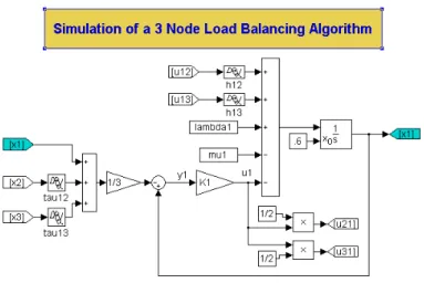
Thetpi’s were taken to be equal. Figure (2) is a block diagram of one node of
the system.
The simulation of the linear model was performed with three nodes (n= 3),
K1 =K2 =K3 =K, pij = 1/2,for alli, j,τij =τ , hij = 2τ fori6=j, τii = 0,
hii = 0fori= 1,2,3andτ = 200µsec. The maximum value for the gain using these parameter values is
Kmax= 5π
4τsin(π/3) =
5π
Figure 2: Simulation Block Diagram for Node 1
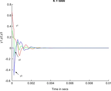
Figures 3 and 4 show the responsesy1(t), y2(t), y3(t)with the gainK= 1000
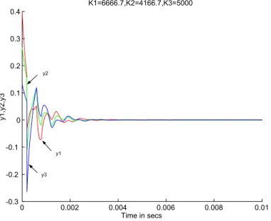
andK= 5000, respectively. Note the increase in oscillatory behavior as the gain is increased. To compare with the experimental results given in Figure 8, Figure 5 shows the output responses with the gains set asK1= 6667, K2= 4167, K3= 5000, respectively. In each of the plots, the effect of delay of 200µsec coming into play att= 200µsecis evident. Note that the responses in 4 with the higher gain die out slower and oscillate more compared to the responses in 3. This is due to the delays in that, if the delays are set to zero, then the response with
0 0.002 0.004 0.006 0.008 0.01 -0.6 -0.4 -0.2 0 0.2 0.4 0.6 0.8 Time in secs y1 ,y 2, y3 y1 y2 y3 K = 1000
Figure 3: Linear output responses withK= 1000.
0 0.002 0.004 0.006 0.008 0.01 -0.6 -0.4 -0.2 0 0.2 0.4 0.6 0.8 Time in secs y1 ,y 2, y3 y1 y2 y3 K = 5000
0 0.002 0.004 0.006 0.008 0.01 -0.3 -0.2 -0.1 0 0.1 0.2 0.3 0.4 Time in secs y1 ,y 2, y3 K1=6666.7,K2=4166.7,K3=5000 y1 y2 y3
Figure 5: Linear simulation withK1 = 6666.7;K2 = 4166.7;K3 = 5000
5
Experimental Results
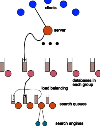
A parallel machine has been built to implement an experimental facility for evaluation of load balancing strategies. To date, this work has been performed for the FBI Laboratory to evaluate candidate designs of the parallel CODIS database. The design layout of the parallel database is shown in Figure 6.
Figure 6: Hardware structure of the parallel database.
A root node communicates with k groups of computer networks. Each of these groups is composed ofn nodes (hosts) holding identical copies of a por-tion of the database. (Any pair of groups correspond to different databases,
which are not necessarily disjoint. A speciÞc record, or DNA proÞle, is in gen-eral stored in two groups for redundancy to protect against failure of a node.) Within each node, there are either one or two processors. In the experimental facility, the dual processor machines use1.6GHz Athlon MP processors, and the single processor machines use1.33GHz Athlon processors. All run the Linux operating system. Our interest here is in the load balancing in any one group ofnnodes/hosts.
The database is implemented as a set of queues with associated search engine threads, typically assigned one per node of the parallel machine. Due to the structure of the search process, search requests can be formulated for any target DNA proÞle and associated with any node of the index tree. These search requests are created not only by the database clients; the search process also creates search requests as the index tree is descended by any search thread. This creates the opportunity for parallelism; search requests that await processing may be placed in any queue associated with a search engine, and the contents of these queues may be moved arbitrarily among the processing nodes of a group to achieve a balance of the load. This structure is shown in Figure 7.
Figure 7: A depiction of multiple search threads in the database index tree. Here the server corresponds to the “root” in Figure 6. To even out the search queues, load balancing is done between the nodes (hosts) of a group. If a node has a dual processor, then it can be considered to have two search engines for its queue.
An important point is that the actual delays experienced by the network traffic in the parallel machine are random. Work has been performed to char-acterize the bandwidth and delay on unloaded and loaded network switches, in order to identify the delay parameters of the analytic models and is reported in [9][10]. The valueτ = 200 µsec used for simulations represents an average
value for the delay and was found using the procedure described in [10]. The in-terest here is to compare the experimental data with that from the three models previously developed.
To explain the connection between the control gain K and the actual im-plementation, recall that the waiting time is related to the number of tasks as
xi(t) =qi(t)tpi wheretpi is the average time to carry out a task. The continuous
time control law is
u(t) =−Kyi(t)
where u(t) is the rate of decrease of waiting time xi(t)per unit time. Conse-quently, the gainKrepresents the rate of reduction of waiting time per second in the continuous time model. Also,yi(t) =
³
qi(t)−³Pnj=1qj(t−τij) ´
/n´tpi =
ri(t)tpi where ri(t) is simply the number of tasks above the estimated (local)
average number of tasks. With∆t the time interval between successive execu-tions of the load balancing algorithm, the control law says that a fraction of the queueKzri(t)(0< Kz<1) is removed in the time∆t so the rate of reduction ofwaiting time is−Kzri(t)tpi/∆t=−Kzyi(t)/∆t so that
u(t) =−Kzyi(t)
∆t =⇒K= Kz
∆t. (9)
This shows that the gainKis related to the actual implementation by how fast the load balancing can be carried out and how much (fraction) of the load is transferred. In the experimental work reported here, ∆t actually varies each time the load is balanced. As a consequence, the value of ∆t used in (9) is an average value for that run. The average timetpi to process a task is the
same on all nodes (identical processors) and is equal10µsec while the time it takes to transfer of load is about 50µsec. The initial conditions were taken as q1(0) = 60000, q2(0) = 40000, q3(0) = 20000 (corresponding to x1(0) =
q1(0)tpi = 0.6, x2(0) = 0.4, x3(0) = 0.2). All of the experimental responses
were carried out with constantpij = 1/2fori6=j.
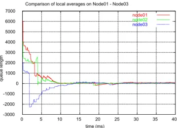
Figure 8 is a plot of the responses ri(t) = qi(t)−³Pnj=1qj(t−τij) ´
/n
for i = 1,2,3 (recall that yi(t) = ri(t)tpi). The (average) value of the gains
were (Kz = 0.5) K1 = 0.5/75µsec = 6667, K2 = 0.5/120µsec = 4167, K3 = 0.5/100µsec = 5000. ThisÞgure compares favorably with Figure 5 of the linear model except for the time scale being off, that is, the experimental responses are slower. The explanation for this it that the gains here vary during the run because ∆t (the time interval between successive executions of the load balancing algorithm) varies during the run. Further, this time∆tisnotmodeled in the continuous time simulations, only its average effect in the gainsKi.That is, the continuous time model does not stop processing jobs (at the average rate
-3000 -2000 -1000 0 1000 2000 3000 4000 5000 6000 7000 0 5 10 15 20 25 30 35 40 q u e u e le n g th time (ms) Comparison of local averages on Node01 - Node03
node01 node02 node03
Figure 8: Experimental response of the load balancing algorithm. The average value of the gains are (Kz = 0.5) K1 = 6667, K2 = 4167, K3 = 5000 with
constantpij.
Figure 9 shows the plots of the response for the (average) value of the gains given by (Kz= 0.2)K1= 0.2/125µsec = 1600, K2= 0.2/80µsec = 2500, K3= 0.2/70µsec = 2857. Note that these gains are about half that of the previous case with a consequence that the response die out slower. The initial condi-tions were q1(0) = 60000, q2(0) = 40000, q3(0) = 20000 (x1(0) = q1(0)tpi =
-3000 -2000 -1000 0 1000 2000 3000 4000 5000 6000 7000 0 5 10 15 20 25 30 35 40 q ue u e le ng th time (ms) Comparison of local averages on Node01 - Node03
node01 node02 node03
Figure 9: Experimental response of the load balancing algorithm. The average value of the gains are (Kz = 0.2) K1 = 16000, K2 = 2500, K3 = 2857 with
constantpij.
Figure 10 shows the plots of the response for the (average) value of the gains given by (Kz = 0.3) K1 = 0.3/125µsec = 2400, K2 = 0.3/110µsec = 7273, K3= 0.3/120µsec = 2500. -3000 -2000 -1000 0 1000 2000 3000 4000 5000 6000 7000 0 5 10 15 20 25 30 35 40 q ue u e le ng th time (ms) Comparison of local averages on Node01 - Node03
node01 node02 node03
Figure 10: Experimental response of the load balancing algorithm. The average value of the gains are (Kz = 0.3) K1 = 2400, K2 = 7273, K3 = 2500 with
6
Summary and Conclusions
In this work, a load balancing algorithm was modeled in three ways using a linear time-delay model. Under the assumption of symmetric nodes and controllers (all intercommunication delays are identical and the controller gains identical) a systematic procedure was presented to determine the stability of the linear system by an explicit relationship between the delay values and the control gain. In particular, the delays create a limit on the size of the controller gains in order to ensure stability. Experiments were performed that indicate a correlation of the continuous time models with the actual implementation.
A consideration for future work is the fact that the load balancing operation involves processor time which is not being used to process tasks. Consequently, there is a trade-offbetween using processor time/network bandwidth and the advantage of distributing the load evenly between the nodes to reduce overall processing time.
An issue is that the delays in actuality are not constant and depend on such factors as network availability, the execution of the software, etc. An approach to modeling using a discrete-event/hybrid state formulation that accounts for block transfers that occur after random intervals may also be advantageous in analyzing the network.
7
Acknowledgements
The work of J.D. Birdwell, V. Chupryna, Z. Tang, and T.W. Wang was sup-ported by U.S. Department of Justice, Federal Bureau of Investigation under contract J-FBI-98-083. Drs. Birdwell and Chiasson were also partially sup-ported by a Challenge Grant Award from the Center for Information Technol-ogy Research at the University of Tennessee. The work of C.T. Abdallah was supported in part by the National Science Foundation through the grant INT-9818312. The views and conclusions contained in this document are those of the authors and should not be interpreted as necessarily representing the official policies, either expressed or implied, of the U.S. Government.
References
[1] C. Abdallah, J. Birdwell, J. Chiasson, V. Churpryna, Z. Tang,
and T. Wang. Load balancing instabilities due to time delays in parallel computation. In “Proceedings of the 3rd IFAC Conference on Time Delay Systems” (December 2001). Sante Fe NM.
[2] R. Bellman and K. Cooke. “Differential-Difference Equations”. New York: Academic (1963).
[3] J. Birdwell, R. Horn, D. Icove, T. Wang, P. Yadav, and S. Niez-goda. A hierarchical database design and search method for codis. In
“Tenth International Symposium on Human IdentiÞcation” (September 1999). Orlando, FL.
[4] J. Birdwell, T. Wang, R. Horn, P. Yadav, and D. Icove. Method of indexed storage and retrieval of multidimensional information. In “Tenth SIAM Conference on Parallel Processing for ScientiÞc Computation” (Sep-tember 2000). U. S. Patent Application 09/671,304.
[5] J. Birdwell, T.-W. Wang, and M. Rader. The university of ten-nessee’s new search engine for codis. In “6th CODIS Users Conference” (February 2001). Arlington, VA.
[6] J. Chiasson. A method for computing the interval of delay values for which a differential-delay system.IEEE Transactions on Automatic Control 33(12), 1176—1178 (December 1988).
[7] J. Chiasson and C. Abdallah. A test for robust stability of time de-lay systems. In “Proceedings of the 3rd IFAC Conference on Time Dede-lay Systems” (December 2001). Sante Fe, NM.
[8] A. Corradi, L. Leonardi, and F. Zambonelli. Diffusive
load-balancing polices for dynamic applications. IEEE Concurrency 22(31), 979—993 (Jan-Feb 1999).
[9] P. Dasgupta. “Performance Evaluation of Fast Ethernet, ATM and Myrinet under PVM, MS Thesis”. University of Tennesse (2001).
[10] P. Dasgupta, J. D. Birdwell, and T. W. Wang. Timing and conges-tion studies under pvm. In “Tenth SIAM Conference on Parallel Processing for ScientiÞc Computation” (March 2001). Portsmouth, VA.
[11] O. Diekmann, S. A. van Gils, S. M. V. Lunel, and H. Walther.
“Delay Equations”. Springer-Verlag (1995).
[12] J. Hale and S. V. Lunel. “Introduction to Functional Differential Equa-tions”. Springer-Verlag (1993).
[13] D. Hertz, E. Jury, and E. Zeheb. Stability independent and dependent of delay for delay differential systems. J. Franklin Institute (September 1984).
[14] E. Kamen. Linear systems with commensurate time delays: Stability and stabilization independent of delay. IEEE Transactions on Automatic Control 27, 367—375 (April 1982).
[15] L. Kleinrock. “Queuing Systems Vol I : Theory”. John Wiley & Sons (1975). New York.
[16] F. Spies. Modeling of optimal load balancing strategy using queuing the-ory. Microprocessors and Microprogramming 41, 555—570 (1996).
[17] T. Wang, J. Birdwell, P. Yadav, D. Icove, S. Niezgoda, and S. Jones. Natural clustering of DNA/STR proÞles. In “Tenth Interna-tional Symposium on Human IdentiÞcation” (September 1999). Orlando, FL.
[18] T. Wang, J. D. Birdwell, P. Yadav, D. J. Icove, S. Niezgoda, and S. Jones. Natural clustering of DNA/STR proÞles. In “Tenth International Symposium on Human IdentiÞcation” (September 1999). Orlando, FL. [19] M. Willebeek-LeMair and A. Reeves. Strategies for dynamic load
balancing on highly parallel computers. IEEE Transactions on Parallel and Distributed Systems 4(9), 979—993 (1993).