Proceedings of the
4th International Workshop on
Multi-Paradigm Modeling
(MPM 2010)
Modelling- and Simulation-Based Design of Multi-tier Systems
Kamal Zellag and Hans Vangheluwe
14 pages
Guest Editors: Vasco Amaral, Hans Vangheluwe, C ´ecile Hardebolle, Lazlo Lengyel Managing Editors: Tiziana Margaria, Julia Padberg, Gabriele Taentzer
Modelling- and Simulation-Based Design of Multi-tier Systems
1Kamal Zellag and1 2Hans Vangheluwe
1McGill University, Montr´eal, Canada 2University of Antwerp, Belgium
Abstract:
This paper introduces a domain-specific language for modelling and simulation-based design of multi-tier systems. Multi-tier systems are complex and very few general models have been developed. Rather, models are always dedicated to a specific architecture. Our approach allows for rapid experimentation with different multi-tier alternatives. Not only parameters, but also structure can be drastically varied. Using graph transformation, multi-tier systems models are translated into
Queueing Petri Nets (QPNs) in a systematic way for analysis with the SimQPN simulator. We describe QPN, our multi-tier architecture visual language, as well as the transformation between them. A case study demonstrates the power of the approach for design-space exploration.
Keywords:Multi-Paradigm Modelling; Meta-Modelling; Multi-tier Systems; Queue-ing Petri Nets; Design-space Exploration.
1
Introduction
Multi-tier architectures have become the standard for advanced information systems. The information system provides services to its connected clients via business methods. The appli-cation server, considered as a middle-tier, is responsible for the method execution. All sensitive data is stored in a database system, called the backend-tier. Whenever a method has to retrieve or update such data, the application server makes the corresponding calls to the database system. In a typical multi-tier architecture [AASM07,WK05,CCE+03], a web-server is often placed between the client and the application server. In this case, clients are often web-browsers, and the web-server is responsible to accept HTTP requests, transform them to calls to the application server, and return the responses of the application server to the client in the form of dynamically generated web-pages. A web-server is also considered a middle-tier component.
Due to the complexity of multi-tier systems, in particular, the complex interactions between their components, it is hard to predict their performance. Hence, simulation-based performance analysis of models of multi-tier systems is highly desirable. Very few models have been de-veloped however. Existing models target a specific architecture of a multi-tier system such as models of the SPECjAppServer2004 benchmark [Kou06]. Alternately, models are quantitative, based on queueing networks [ZR06].
The choice of QPNs as a semantic domain allows for both quantitative and qualitative analysis of the modelled system. The behaviour of each type of component in a multi-tier system, such as database server, application server, or load balancer, is provided in the form of a QPN. In our framework, the domain-specific multi-tier models are automatically transformed into complete QPN models for performance analysis.
In this work, we develop visual modelling languages using our meta-modelling and model transformation environment AToM3 [LV02]. The first is a multi-tier architecture description language. The second is a QPN modelling language. We use graph transformation models to explicitly describe and subsequently execute the transformations between both. We export the QPN models in XML format for use in the SimQPN [KB06] discrete-event simulator.
The paper is organized as follows: In section 2, an overview of somePetri Netvariants leads toQueueing Petri Nets. Section 3 presents our two modelling languages and uses them to model a typical multi-tier system. Section 4 presents the rule-based transformation from the multi-tier model to the QPN model. Section 5 presents some of the simulations results. This leads to simulation-based design-space exploration. Finally, conclusions and future work are presented in Section 6.
2
Queueing Petri Nets
In this section we briefly describe the Queueing Petri Nets formalism. We start from simple Place/Transition Petri Nets then we gradually add extra features.
Place/Transition Petri Nets
Place/TransitionPetri Nets(P/T PNs) are a formalism for describing the behaviour of concur-rent asynchronous processes. They allow for an elegant description of synchronization.
A P/T PN is a bipartite directed graph composed of places and transitions [BK02]:
PN= (P,T,I−,I+,M
0),where:
1. P is a finite and non-empty set of places. 2. T is a finite and non-empty set of transitions. 3. P∩T =/0.
4. I−,I+:P×T→N0are the backward and forward incidence functions.
5. M0:P→N0is the initial marking.
The interconnections between places and transitions are specified by the incidence functions
I− and I+. If I−(p,t)>0, an arc connects a place p to transition t and place p is called an input place of the transition. IfI+(p,t)>0, an arc connects a transitiont to place pand place
p is called an output place of the transition. Each arc has a weight which is a natural number given by the incidence function. The initial distribution of tokens in the net (called marking) is given by the functionM0which specifies how many tokens are contained in each place. The
Coloured Petri Nets
Coloured Petri Nets (CPNs) [BK02] are an extension to P/T PNs whereby each token has a colour property. A set of colours is assigned to each place by a colour function. This set specifies the types of tokens that are accepted in this place. For each transitiont in a CPN, a guard function, providing a set of first-order formulas over the colours of tokens, defines firing modes for t.
Generalized Stochastic Petri Nets
Another extension to P/T PNs areGeneralized Stochastic Petri Nets(GSPNs). Transitions in GSPNs can be immediate or timed. The immediate transitions can be fired once they are enabled, while the timed transitions have to wait for a certain amount of time before firing. This time is generally defined as an exponentially distributed function. If many immediate transitions are enabled at the same time, the next transition to fire is selected based on firing weights assigned to the transitions. The firing of immediate transitions always has priority over that of timed transitions.
AGeneralized Stochastic Petri Netis defined as a 4-tupleGSPN= (PN,T1,T2,W),where:
1. PN= (P,T,I−,I+,M0) is the underlying P/T Petri Net.
2. T1⊆T is the set of timed transitions, T16= /0
3. T2⊂T is the set of immediate transitions, T1∩T2=/0,T =T1∪T2
4. W = (w1, ...,w|T|)is an array whose entry wi∈R+:
- is a rate of a negative exponential distribution specifying the firing delay, when transition tiis a timed transition
- is a firing weight, when transition tiis an immediate transition
Coloured Generalized Stochastic Petri Nets(CGSPNs) [DCB88] are defined by the combina-tion of CPNs and CGPNs.
Queueing Networks
A Queueing Network (QN) consists of a collection of service stations and customers. The service stations represent system resources while the customers represent users or transactions.
Figure 1: A Service Station A service station (see Figure1) is composed
of one or more servers and a waiting area. When a request arrives at a service station, it is immediately serviced if a free server is avail-able. Otherwise, the request has to wait in the waiting area. Different scheduling strate-gies [BGMT98] can be used to serve the re-quests waiting in the waiting area. Some typ-ical scheduling strategies are:
• FCFS (First-Come-First-Served): Requests are served in order of arrival.
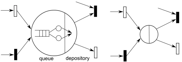
Figure 2: A Queued Place and its shorthand notation
• PS (Processor-Sharing): Requests are assumed to be served simultaneously with the server being equally shared among them.
Queueing Petri Nets
CombiningColoured Generalized Stochastic Petri Nets(CGSPNs) withQueueing Networks
(QNs) yields a modelling formalism called Queueing Petri Nets (QPNs) [Bau93]. Places in QPNs are of two types: ordinary and queued. A queued place (see Figure2) is composed of a queue (service station) and a depository. After being served by the service station, (coloured) tokens are placed onto the depository. Tokens, when fired onto a queued place by any of its input transitions, are inserted into the queue according to the scheduling strategy of the queue. Tokens in the queue are not available for output transitions while tokens in the depository are available to all output transitions of the queued place. White rectangles in Figure2 represent timed transitions while black rectangles represent immediate transitions.
3
Modelling multi-tier systems
Anecdotal evidence shows that domain-specic modelling (DSM) can lead to drastic increase in productivity [KT08]. DSM raises the level of abstraction if it is used properly by the user. Using Domain-Specific Visual Languages (DSVLs) in particular, designers are provided with high-level, intuitive notations which allow them to build models with concepts of the domain without dealing with low level details.
Multi-tier Model
Figure 3: A a sample architecture in our multi-tier DSVL
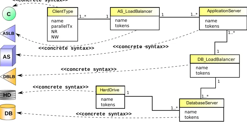
Figure 4: Multi-tier DSVL abstract and concrete syntax
The abstract syntax of our multi-tier DSVL is specified using a Class Diagram meta-model as shown in Figure4 (constraints omitted). In the figure, the concrete syntax of the DSVL is given linking visual representations to the different abstract syntax elements (concrete syntax of associations omitted).
In this article, we use AToM3, A Tool for Multi-formalism and Meta-Modelling [LV02] for all modelling, meta-modelling and model transformation.
QPN Model
Multi-tier model representations as described above are sufficient to specify system structure. Due to the high level of abstraction, the system’s behaviour is however not readily inferred.
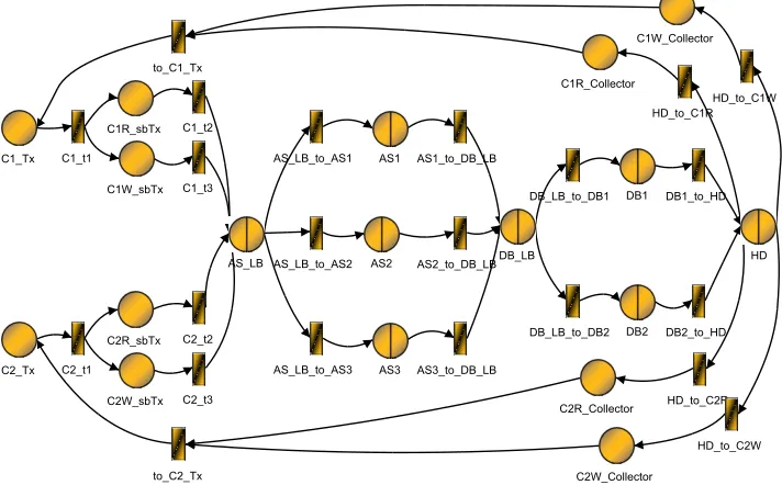
and concrete syntax of) a QPN visual language. Figure5shows our QPN model for the sample multi-tier architecture from Figure3. Each server in this architecture is modelled as a queueing
Figure 5: A QPN Model for the sample multi-tier architecture
place. Queueing places with more than one server can be used but for simplicity we assume that all are limited to one server. Rather than modelling each client separately, we classify clients according to their transaction type, which leads to different categories of clients. In a multi-tier system, transactions can be divided into many sub-transactions. These can in turn be divided into read-only or write-only sub-transactions. We encode these different types as QPN colours. For each client transaction, this leads to three coloured tokens. The first token (C) represents the global transaction initiated by the client. The second (CR) and the third (CW) represent the read-only and write-only sub-transactions respectively. At this point, we have defined the queued places and the coloured tokens in our model, but we still have to define the transitions and their firing modes. Let’s assume that for a class C of clients, a transaction is initiated. This transaction contains NR read-only sub-transactions and NW write-only sub-transactions. This will define the firing weights of transitions on the client side. In our QPN model, the transitions C1 t1 and C2 t1 define the firing weights for each transaction initiated by a client of type C1. The transitions to C1 Tx and to C2 Tx are used to control the number of parallel transactions of the class C1 running at the same time. The transition to C1 Tx will fire only if it receives NR tokens of the colour CR and NW tokens of the colour CW. The ordinary place C1 is initiated with the number of parallel transactions of class C1 running at the same time. Each queued place is parametrized with accepted coloured tokens and some data related to the time needed by the server to process each of these tokens.
4
Model Transformation: mapping multi-tier onto QPN
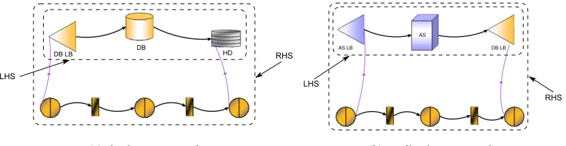
domain-(a) database server rule (b) application server rule
Figure 6: Transformation rules for servers
specific model, highlights the structure of a multi-tier architecture and can rapidly be constructed by a designer. The second, QPN model, gives a detailed specification of the behaviour (assuming QPN semantics is known). We now provide semantic anchoring of the multi-tier formalism by providing a mapping between a multi-tier model and a corresponding QPN model, for all models in the multi-tier DSVL.
This approach has several advantages. On the one hand, it cleanly separates the two lan-guages: the designer of multi-tier systems need not know (and is unlikely to know) about the QPN formalism, yet, thanks to the mapping, a QPN model can be automatically generated for each multi-tier model. This allows for performance analysis through simulation. Note that in this setup it is necessary to provide trace-ability: backward links from the QPN model (and sim-ulation results) to the context of the multi-tier domain model. On the other hand, the approach allows for the structured variation of the mapping. This could be to other formalisms (such as DEVS for detailed discrete-event simulation) or target platform languages (in case multi-tier ap-plication synthesis is desired). The mapping could also be modified to encode other detailed design choices such as the use of thread pools (as will be demonstrated later on).
We choose to model the multi-tier to QPN mapping explicitly, in a rule-based fashion, based on graph transformation. This approach is structured, which makes it easy to understand and re-use. It also ties in nicely with the meta-models of both source and target formalism.
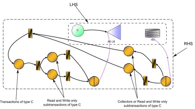
We define an ordered (by priority) collection of transformation rules using AToM3. These rules are represented using the concrete syntax of source- and target languages. Each rule contains a left hand side (LHS) and a right hand side (RHS) model pattern. A “match” of the LHS pattern in the (to be transformed) host model is searched for. Elements which appear in the LHS but not in the RHS of a rule are deleted. Elements which appear in the RHS but not in the LHS of a rule are deleted. Elements which appear in both LHS and RHS are retained. Post-rule-application model attribute values can be specified based on pre-rule-application attribute values. A few multi-tier to QPN rules are shown to illustrate the approach.
Figure 7: Transformation rule for a class of clients of category C
and the DB load balancer). Figure 7 shows another transformation rule which transforms a class of clients to its equivalent components in the QPN model. As explained before, each transaction initiated by a client of class C generates NR read-only sub-transactions and NW write-only sub-transactions. On the left of the figure, three ordinary places and three firing transitions are generated. From the hard drive queued place (on the right side of the figure), read-only and write-only sub-transactions are collected and then sent back to their original place which subsequently generates a new transaction in the system. Those NR read-only and NW write-only sub-transactions are removed from their places only if there are more than NR and NW tokens in the collector places respectively. As intended, the transformation results in the model previously constructed by hand, shown in Figure5. Not only is the transformation-based approach less error prone, the domain-expert’s mapping knowledge is now explicitly represented in the transformation model.
The rule-based approach also allows for modular modification of the behaviour/realization of a multi-tier architecture. Figure8shows a modified version of the transformation rule in part(a)
of Figure6. On the RHS, we add a place representing the thread pool of the database server. This place contains initially a number of tokens which represents the maximum number of available parallel threads handling sub-transactions on the database server. Figure9shows the impact of the minimal modification of one rule on the full transformation from the multi-tier model to the QPN model. Two places, TP DB1 and TP DB2, were generated for the database servers DB1 and DB2 respectively. Note that both source and target models appear, with some traceability links. This is not surprising as the rules did not delete source model elements.
5
Simulation-based Design-space Exploration
Figure 8: Transformation rule for a database server with a Thread Pool place
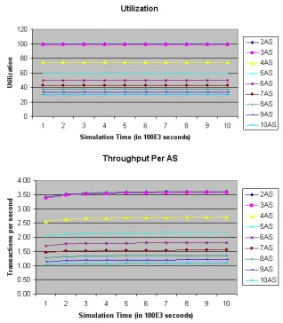
Figure 11: Utilization and throughput of each Application Server
Figure 10: Design-space exploration as shown in Figure10. We now present some
simulations results for the multi-tier archi-tecture shown in Figure 3. We varied the number of application servers in the 2 to 10 range and performed several simulation runs for each of these architectures. Using multiple runs is necessary to verify statistical proper-ties of the obtained performance metrics. Fig-ure11shows the utilization (%) and through-put (1/s) of each application server in each multi-tier architecture. Thex-axis of these fig-ures presents the simulation time. The
Figure 12: Overall Throughput of all Application Servers
conclude that a simulated run-time above 105sis sufficient to obtain relevant results. We notice that as the number of application servers increases, the utilization and throughput decrease. This was expected since the application server load balancer in our models uses a fair load distribution among all application servers.
The utilization of an application server can help a designer to decide which architecture satis-fies some desired performance requirements. Another metric that can be useful in such decisions is the overall throughput of all application servers. It is equal to the sum of the throughputs of all application servers. Figure12shows this value for all architectures used in our simulations. In this figure, we notice that there is no apparant benefit of using more than three application servers. Based on the utilization of each application server and the overall throughput in each simulation, we can define performance criteria to help select the optimal architecture. We wish to use each application server as intensely as possible but without exceeding critical load limits where the application server becomes a bottleneck. It is common for a multi-tier system designer to target 70% as utilization for each application server and maximize the overall throughput of all application servers. This leads us to maximize the following function:
f(util,oT hr) =oT hr/ABS(util−70)
where:
-util: stands for the application server utilization, and -oThr: stands for the overall throughput.
Adding a new application server is costly in terms of hardware as well as software licenses. For simplicity, we assume that this cost is a linear function of the number of application servers (NAS). By using this parameter, our new objective function to maximize becomes:
g(util,oT hr,NAS) = f(util,oT hr)/NAS
Figure 13: Values of thegObjective Function
Note that to arrive at this conclusion, a designer only needs to build and modify multi-tier architecture models. Generation of QPN models, simulation, and collection of performance metrics is fully automated. Even though running the simulations takes several hours per design alternative, the designer’s effort is minimal. Furthermore, the whole process is traceable and repeatable. If necessary, a domain expert may modify the transformation model, again with minimal effort. For those designers who had the expertise to do simulation-based performance analysis, this greatly simplifies the process, and eliminates mistakes. For designers who did not have the expertise, simulation-based performance analysis now comes within reach.
6
Conclusions and Future Work
Bibliography
[AASM07] S. Agarwala, F. Alegre, K. Schwan, J. Mehalingham. E2EProf: Automated End-to-End Performance Management for Enterprise Systems. InDSN ’07: Proceedings of the 37th Annual IEEE/IFIP International Conference on Dependable Systems and Networks. Pp. 749–758. 2007.
[Bau93] F. Bause. Queueing Petri Nets: A Formalism for the Combined Qualitative and Quantitative Analysis of Systems. InThe 5th International Workshop on Petri Nets and Performance Models. Pp. 14 – 23. 1993.
[BGMT98] G. Bolch, S. Greiner, H. de Meer, K. S. Trivedi.Queueing networks and Markov chains: modeling and performance evaluation with computer science applications. Wiley, 1998.
[BK02] F. Bause, F. Kritzinger.Stochastic Petri Nets - An Introduction to the Theory. Vieweg Verlag, 2002.
[CCE+03] E. Cecchet, A. Chanda, S. Elnikety, J. Marguerite, W. Zwaenepoel. Performance comparison of middleware architectures for generating dynamic Web content. In
Middleware. Pp. 242–261. 2003.
[DCB88] T. Demaria, G. Chiola, G. Bruno. Introducing a color formalism into Generalized Stochastic Petri nets. InThe 9th International Workshop on Application and Theory of Petri Nets. Pp. 202 – 215. 1988.
[KB06] S. Kounev, A. Buchmann. SimQPN: a tool and methodology for analyzing Queue-ing Petri Net models by means of simulation.Perform. Eval.63(4):364–394, 2006.
[Kou06] S. Kounev. Performance Modeling and Evaluation of Distributed Component-Based Systems Using Queueing Petri Nets.IEEE Transactions on Software Engineering
32(7):486–502, 2006.
[KT08] S. Kelly, J.-P. Tolvanen.Domain-Specific Modeling: Enabling Full Code Genera-tion. Wiley, 2008.
[LV02] J. de Lara, H. Vangheluwe. AToM3: A Tool for Multi-formalism and Meta-Modelling. In European Joint Conference on Theory And Practice of Software (ETAPS), Fundamental Approaches to Software Engineering (FASE). LNCS 2306, pp. 174 – 188. Springer, 2002.
[WK05] H. W. Wu, B. Kemme. Fault-tolerance for Stateful Application Servers in the Pres-ence of Advanced Transactions Patterns. In SRDS ’05: Proceedings of the 24th IEEE Symposium on Reliable Distributed Systems. Pp. 95–108. IEEE, 2005.