Proceedings of the
XIII Spanish Conference on Programming
and Computer Languages
(PROLE 2013)
R-SQL: An SQL Database System with Extended Recursion
1Gabriel Aranda, Susana Nieva, Fernando S´aenz-P´erez and Jaime S´anchez-Hern´andez
18 pages
Guest Editors: Clara Benac Earle, Laura Castro, Lars- ˚Ake Fredlund Managing Editors: Tiziana Margaria, Julia Padberg, Gabriele Taentzer
ECEASST Home Page: http://www.easst.org/eceasst/ ISSN 1863-2122
TIN2008-R-SQL: An SQL Database System with Extended Recursion
†Gabriel Aranda1, Susana Nieva1, Fernando S´aenz-P´erez2and Jaime S´anchez-Hern´andez1
1Dept. Sistemas Inform´aticos y Computaci´on, UCM, Spain 2Dept. Ingenier´ıa del Software e Inteligencia Artificial, UCM, Spain [email protected], [email protected], [email protected], [email protected]
Abstract:
The relational database language SQL:1999 standard supports recursion, but this approach is limited to the linear case. Moreover, mutual recursion is not supported, and negation cannot be combined with recursion. We designed the language R-SQL to overcome these limitations in [ANSS13], improving termination properties in re-cursive definitions. In addition we developed a proof of concept implementation of an R-SQL system. In this paper we describe in detail an improved system enhanc-ing performance. It can be integrated into existenhanc-ing RDBMS’s, extendenhanc-ing them with the aforementioned benefits of R-SQL. The system processes an R-SQL database definition obtaining its extension in tables of an RDBMS (such as PostgreSQL and DB2). It is implemented in SWI-Prolog and it produces a Python script that, upon execution, computes the result of the R-SQL relations. We provide some perfor-mance results showing the efficiency gains w.r.t. the previous version. We also include a comparative analysis including some representative relational a deductive systems.
Keywords:Databases, SQL, Recursion, Fixpoint Semantics
1
Introduction
Recursion is a powerful tool nowadays included in almost all programming systems. However, for current implementations of the declarative programming language SQL, this tool is heavily compromised or even not supported at all (MySQL, MS Access, . . . ) Those systems including recursion suffer from several drawbacks. Linearity is required, so that relation definitions with calls to more than one recursive relation are not allowed. Mutual recursion, and query solving involving an EXCEPT clause are not supported. In general, termination is manually controlled by limiting the number of iterations instead of detecting that there are no further opportunities to develop new tuples. Duplicate discarding is not supported and, so, queries that are actually terminating are not detected as such.
Starburst [MP94] was the first non-commercial RDBMS to implement recursion whereas IBM DB2 was the first commercial one. ANSI/ISO Standard SQL:1999 included for the first time
†This work has been partially supported by the Spanish projects TIN2013-44742-C4-3-R (CAVI-ART),
recursion in SQL. Today, we can find recursion in several systems: IBM DB2, Oracle, MS SQL Server, HyperSQL and others with the aforementioned limitations.
In [ANSS13] we proposed a new approach, called R-SQL, aimed to overcome these limita-tions and others, allowing in particular cycles in recursive definilimita-tions of graphs and mutually recursive relation definitions. In order to combine recursion and negation, we applied ideas from the deductive database field, such as stratified negation, based on the definition of a dependency graph between the relations involved in the database [Ull89]. We developed a formal framework following the original relational data model [Cod70], therefore avoiding both duplicates and nulls (as encouraged by [Dat09]). We used a stratified fixpoint semantics and we presented an R-SQL database system as a prototype implementing such formal framework. The system can be down-loaded from https://gpd.sip.ucm.es/trac/gpd/wiki/GpdSystems/RSQL. In this work, we describe in detail an improved version enhancing performance. The system processes an R-SQL database definition obtaining its extension in tables of an RDBMS (such as PostgreSQL and DB2). It is implemented in SWI-Prolog and it generates a Python script that, upon execution, computes the result of the R-SQL relations. The improvements in effi-ciency relies on a new stratification and a more elaborated version of the fixpoint calculation algorithm that allows to avoid recomputations along iterations. The new system is available athttps://gpd.sip.ucm.es/trac/gpd/wiki/GpdSystems/RSQLplus. In addi-tion, we experiment with some previously proposed optimizations [Ull89] to improve the perfor-mance of the fixpoint computation.
Related academic approaches includeDLVDB[TLLP08], LDL++ [AOT+03] (now abandoned and replaced by DeALS, which does not refer to SQL queries up to now), and DES [SP13]. The first one, resulting of a spin-off at Calabria University, is the closer to our work as it produces SQL code to be executed in the external database with a semi-na¨ıve strategy, but lacks formal support for its proposal, and it does not describe non-linear recursion. Last two ones also allow connecting to external databases, but processing of recursive SQL queries are in-memory.
The paper is organized as follows: In Section2we recall the syntax and the meaning of R-SQL database definitions. Section 3 describes the system, including the new form of stratification, the fixpoint algorithm, and some performance measurements, showing the efficiency gains for several optimizations. We also include a comparative analysis including some representative relational and deductive systems. Conclusions and future work are summarized in Section4.
2
Introducing R-SQL
In this section, we present an overview of the language R-SQL, which is focused on the incor-poration of recursive relation definitions. The idea is simple and effective: A relation is defined with an assignment operation as a named query (view) that can contain a self reference, i.e., a relationRcan be defined asR sch:=SELECT. . .FROM. . .R. . ., whereschis the relation schema.
2.1 The Definition Language of R-SQL
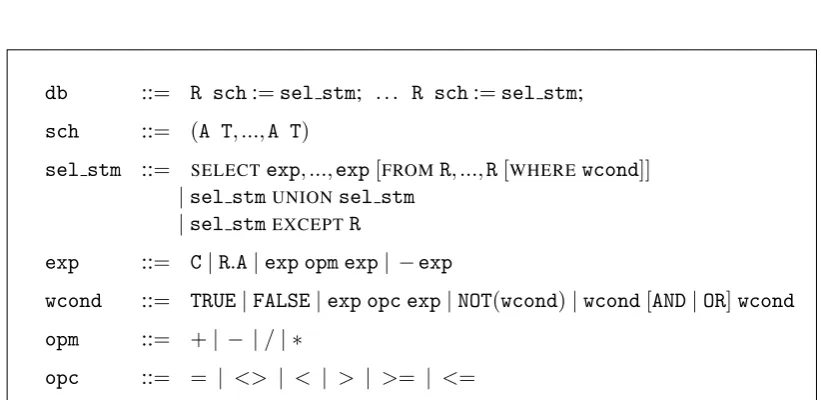
db ::= R sch:=sel stm; . . . R sch:=sel stm;
sch ::= (A T, ...,A T)
sel stm ::= SELECTexp, ...,exp[FROMR, ...,R[WHEREwcond]]
|sel stmUNIONsel stm |sel stmEXCEPTR
exp ::= C|R.A|exp opm exp| −exp
wcond ::= TRUE|FALSE|exp opc exp|NOT(wcond)|wcond[AND|OR]wcond opm ::= +| − |/| ∗
opc ::= = | <> | < | > | >= | <=
Rstands for relation names, A for attribute names, T for standard SQL types and C for constants belonging to a valid SQL type.
Figure 1: A Grammar for the R-SQL Language
use small caps). As usual, optional statements are delimited by square brackets and alternative sentences are separated by pipes.
The language R-SQL overcomes some limitations present in current RDBMS’s following SQL:1999. These languages useNOT IN andEXCEPTclauses to deal with negation, and WITH
RECURSIVEto engage recursion. As it is pointed out in [GUW09], SQL:1999 does not allow an
arbitrary collection of mutually recursive relations to be written in theWITH RECURSIVEclause. A bundle of R-SQL database examples can be found with the system distribution. Next, we present some of them, to show the expressiveness of the definition language. Each of them is intended to illustrate a concrete aspect of the language in a simple and concise way. Section3
explores a larger and more natural example.
Mutual Recursion Although any mutual recursion can be converted to direct recursion by inlining [KRP93], our proposal allows to explicitly define mutual recursive relations, which is an advantage in terms of program readability and maintenance. For instance, the following R-SQL database defines the relationsevenandodd, as the classical specification of even and odd numbers up to a bound (100 in the example):
even(x float) := SELECT 0 UNION SELECT odd.x+1 FROM odd WHERE odd.x<100;
odd(x float) := SELECT even.x+1 FROM even WHERE even.x<100;
Nonlinear Recursion The standard SQL restricts the number of allowed recursive calls to be only one. Here we show how to specify Fibonacci numbers in R-SQL1:
fib1(n float, f float) := SELECT fib.n, fib.f FROM fib;
fib2(n float, f float) := SELECT fib.n, fib.f FROM fib;
fib(n float, f float) := SELECT 0,1 UNION SELECT 1,1 UNION SELECT fib1.n+1,fib1.f+fib2.f FROM fib1,fib2
WHERE fib1.n=fib2.n+1 AND fib1.n<10;
Duplicates and Termination Non termination is another problem that arises associated to re-cursion when coupled with duplicates. For instance, the following standard SQL query (that considers a finite relationt) makes current systems either to reject the query or to go into an infinite loop (some systems allow to impose a maximum number of iterations as a simple termi-nation condition, as DB2):
WITH RECURSIVE v(a) AS SELECT * FROM t UNION ALL SELECT * FROM v SELECT * FROM v
Nevertheless, the fixpoint computation for the corresponding R-SQL relation:
v(a float) := SELECT * FROM t UNION SELECT * FROM v;
guarantees termination because duplicates are discarded2 and vdoes not grow unbounded. The very same termination problem also happens in current RDBMS’s with the basic transitive closure over graphs including cycles, but not in R-SQL which ensures termination for finite graphs.
2.2 The meaning of an R-SQL database definition
In [ANSS13] we formalized an operational semantics for the language R-SQL based on stratified negation and fixpoint theory, here we summarize the main ideas.
Stratification is based on the definition of adependency graph DGdbfor an R-SQL database
db that is a directed graph whose nodes are the relation names defined in db, and the edges, that can be negatively labelled, are determined as follows. A relation definition of the form
R sch:=sel stmindbproduces edges in the graph from every relation name insidesel stm
to R. Those edges produced by the relation name that is just to the right of an EXCEPT are negatively labelled.
If there arenrelations defined indb, and we denote byRNthe set of the relation names defined indb, astratificationofdbis a mappingstr:RN→ {1, . . . ,n}, such that for every two relations
R1,R2∈RNit satisfies:
• str(R1)≤str(R2), if there is a path fromR1toR2inDGdb,
• str(R1)<str(R2) if there is a path from R1 to R2 in DGdb with at least one negatively
labelled edge.
2Note that
An R-SQL databasedbisstratifiableif there exists a stratification for it. We denote bynumStr the maximum stratum of the elements ofRN.
Intuitively, a relation name preceded by anEXCEPToperator plays the role of a negated pred-icate (relation) in the deductive database field. A stratification-based solving procedure ensures that when a relation that contains anEXCEPTin its definition is going to be calculated, the mean-ing of the inner negated relation has been completely evaluated, avoidmean-ing nonmonotonicity, as it is widely studied in Datalog [Ull89].
We say that an interpretation I is the relationship between every relation name Rand its in-stance I(R). Interpretations are classified by strata; an interpretation belonging to a stratum i gives meaning to the relations of strata less or equal to i. If I1, I2 are two interpretations of stratum i, we say I1 is less or equal than I2 at stratum i, denoted by I1vi I2, if the following conditions are satisfied for everyR∈RN:
• I1(R) =I2(R), ifstr(R)<i.
• I1(R)⊆I2(R), ifstr(R) =i.
The meaning of everysel stm w.r.t. an interpretationI can be understood as the set of tu-ples (in the current instance represented by I) associated to the corresponding equivalentRA -expression, denoted by[sel stm]I. ThisRA-expression is defined as follows:3
• [SELECTexp1, . . . ,expk FROMR1, . . . ,RmWHEREwcond]I=
πexp1,...,expk(σwcond(I(R1)×. . .×I(Rm)))
• [sel stm1UNIONsel stm2]I= [sel stm1]I∪ [sel stm2]I
• [sel stmEXCEPTR]I= [
sel stm]I−I(
R)
Example1 Consider the definitions of the relationsoddandevenof Section2. Let us assume a concrete interpretationIsuch thatI(even) ={(0),(2)}andI(odd) =/0. Hence, the interpretation of the select statement that defines the relationoddw.r.t.I is:
[SELECT even.x+1 FROM even WHERE even.x<100]I=
{(even.x+1)[a/even.x]|(a)∈I(even),(even.x<100)[a/even.x]is satisfied}=
{(1),(3)}
The case of the relationevenis analogous:
[SELECT 0 UNION SELECT odd.x+1 FROM odd WHERE odd.x<100]I=
[SELECT 0]I∪ [SELECT odd.x+1 FROM odd WHERE odd.x<100]I=
{(0)} ∪ {(odd.x+1)[a/odd.x]|(a)∈I(odd),(odd.x<100)[a/odd.x]is satisfied}=
{(0)}
Notice that the interpretation ˆIdefined by:
ˆ
I(even) ={(0),(2), . . . ,(100)}and ˆI(odd) ={(1),(3), . . . ,(99)}
3Notice that arithmetic expressions are allowed as arguments inprojection(
satisfies: ˆ
I(even) = [SELECT 0 UNION SELECT odd.x+1 FROM odd WHERE odd.x<100]Iˆ ˆ
I(odd) = [SELECT even.x+1 FROM even WHERE even.x<100]Iˆ
So, to give meaning to a database definition, we are interested in an interpretation, called f ix, such that for every R∈RN, if sel stm is the definition ofR, then f ix(R) = [sel stm]f ix. In the previous example f ix will be ˆI. SinceRcan occur inside its definition, for every stratumi, the appropriate interpretation f ixi that gives the complete meaning to each relation of stratum iis the least fixpoint of a continuous operator. These fixpoint interpretations are sequentially constructed from stratum 1 tonumStr. f ixrepresents the fixpoint of the last stratum and provides the semantics for the whole database.
For everyi, 1≤i≤numStr, we define the continuous operatorTi that transforms interpreta-tions belonging to a stratumias follows:
• Ti(I)(R) =I(R), ifstr(R)<i.
• Ti(I)(R) = [sel stm]I, ifstr(R) =iandR sch:=sel stmis the definition ofRindb.
• Ti(I)(R) =/0, ifstr(R)>i.
The operatorT1 has a least fixpoint, which is
F
n≥0T1n(/0), where /0(R) = /0 for every R∈RN. We will denoteF
n≥0T1n(/0)by f ix1, i.e., f ix1represents the least fixpoint at stratum 1.
Consider now the sequence{T2n(f ix1)}n≥0of interpretations of stratum 2, greater than f ix1. Using the definition ofTiand the fact that f ix1(R) =/0 for everyRsuch thatstr(R)≥2, it is easy to prove, by induction onn≥0, that this sequence is a chain:
f ix1v2T2(f ix1)v2T2(T2(f ix1))v2. . .v2T2n(f ix1), . . .
{T2n(f ix1)}n≥0 is a chain that has as least upper bound,
F
n≥0T2n(f ix1), which is the least fixpoint ofT2containing f ix1. We denote this interpretation by f ix2. By proceeding successively in the same way it is possible to find f ixnumStr. In [ANSS13] we have proved that f ixnumStris the interpretation f ixwe are looking for, that associates the set of tuples denoted by its definition to every relation of the database .
3
The Improved R-SQL System
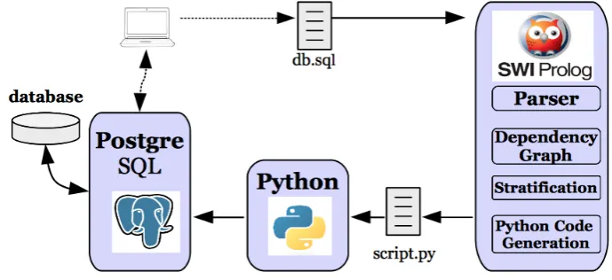
Here we present the R-SQL system, which is based on the fixpoint construction of the previous section. We describe its structure, focusing on the improvements that increase the efficiency of the previous prototype, presented in [ANSS13]. These enhances are essentially due to the stratification described in Section3.1and in the factoring-out process incorporated in the fixpoint algorithm presented in Section3.2.
the RDBMS in order to query or modify the database. Although we are referring to Post-greSQL in the concrete implementationhttps://gpd.sip.ucm.es/trac/gpd/wiki/ GpdSystems/RSQLplus, it can be straightforwardly applied to other systems.
Figure 2: R-SQL System Structure.
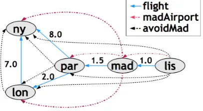
Next we present a database for flights to illustrate the process and also will be the working example for the rest of the section. As usual, the information about direct flights can be composed of the city of origin, the city of destination, and the length of the flight. Cities (Lisbon, Madrid, Paris, London, New York) will be represented with constants (lis,mad,par,lon,ny, resp.). The relationreachable consists of all the possible trips between the cities of the database, maybe concatenating more than one flight. The relation travelis analogous but also gives time information about alternative trips.
flight(frm varchar(10), to varchar(10), time float) := SELECT ’lis’,’mad’,1.0 UNION SELECT ’mad’,’par’,1.5 UNION SELECT ’par’,’lon’,2.0 UNION SELECT ’lon’,’ny’,7.0 UNION SELECT ’par’,’ny’,8.0;
reachable(frm varchar(10), to varchar(10)) := SELECT flight.frm, flight.to FROM flight UNION
SELECT reachable.frm, flight.to
FROM reachable,flight WHERE reachable.to = flight.frm;
travel(frm varchar(10), to varchar(10), time float) :=
SELECT flight.frm, flight.to, flight.time FROM flight UNION SELECT flight.frm, travel.to, flight.time+travel.time
FROM flight, travel WHERE flight.to = travel.frm;
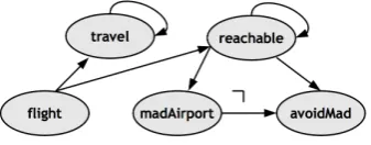
Figure 3:DGdbof the working example.
with arithmetic expressions). The relationmadAirportcontains travels departing or arriving in Madrid, whileavoidMadcontains the possible travels that neither begin, nor end in Madrid.
madAirport(frm varchar(10), to varchar(10)) := SELECT reachable.frm, reachable.to FROM reachable WHERE (reachable.frm = ’mad’ OR reachable.to = ’mad’);
avoidMad(frm varchar(10), to varchar(10)) :=
SELECT reachable.frm, reachable.to FROM reachable EXCEPT madAirport;
This definition includes negation together with recursive relations. This combination can not be expressed in SQL:1999 as it is shown in [FMMP96]. The dependency graph of this database is depicted in Figure3, where negatively labelled edges are annotated with¬.
3.1 Stratification
Given a database and its dependency graph, there can be a number of different stratifications for it. For instance, for the dependency graph of Figure4a possible stratification can assign stratum 1 to the relations{a,b,c,d,e}and stratum 2 to{f,g}.
For the graph of Figure4, intuitively it is easy to see that onlybandcmust belong to the same stratum due to the mutual dependency between them. The next algorithm minimizes the number of relations in each stratum, which allows to enhance the efficiency of the fixpoint computation as shown in Section3.2.
• Compute thestrongly connected components C fromDGdb. Negative labels are not rel-evant initially, but once the components are evaluated, it must be checked if there exists some cycle with a negatively labeled edge. In such a case,dbis not stratifiable and the computation stops. For the example of Figure4the components are{a},{f},{g},{b,c},
{d}and{e}.
¬ a
c b
e d
g f
• Collapse each strongly connected componentobtaining a new graph with a node for each component,C, and with an edge fromCtoC0 if and only ifCcontains a relationRandC0 contains a relationR0, such that there is an edge fromRtoR0inDGdb. In our example, the component{b,c}can be collapsed to the nodebc, and the rest to its single element. The new graph has the edges{a→bc,bc→d,bc→e,a→f,f→g}.
• Obtain atopological sortingfor the resulting graph. In our example we can get the sorting
a<f<g<bc<e<d.
• Uncollapse the nodes of such a sorting for obtaining a topological sorting for the strongly connected components, and enumerate them in ascending order. In our example, we get
{a}<{f}<{g}<{b,c}<{e}<{d}.
Then, the expected stratificationstr(a) =1; str(f) =2; str(g) =3; str(b) =str(c) =
4;str(e) =5; str(d) =6 is obtained.
The concrete implementation of this algorithm in R-SQL uses the library ugraphs of SWI-Prolog and the modulescc implemented by Markus Triska, accessible from http://www. logic.at/prolog/scc.pl. For the dependency graph of Figure3, R-SQL assigns stratum 1 toflight, 2 totravel, 3 toreachable, 4 tomadAirport, and 5 toavoidMad.
3.2 The Computation of the Database Fixpoint
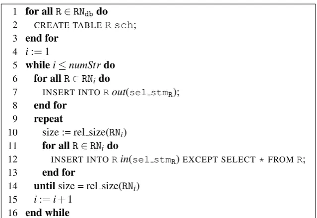
Next, we present the algorithm for generating the SQL database corresponding to the fixpoint of an R-SQL database definitiondb. This algorithm is shown in Figure5. It produces the SQL statements (CREATEandINSERT) needed to build such a database.
1 for allR∈RNdbdo
2 CREATE TABLER sch;
3 end for 4 i:=1
5 whilei≤numStrdo 6 for allR∈RNido
7 INSERT INTORout(sel stmR);
8 end for 9 repeat
10 size := rel size(RNi) 11 for allR∈RNido
12 INSERT INTORin(sel stmR)EXCEPT SELECT*FROMR;
13 end for
14 untilsize = rel size(RNi) 15 i:=i+1
16 end while
The algorithm considers a concrete stratification for the database where numStrdenotes the number of strata andNRi the set of relations of stratumi. First of all, a table is created for each relation R sch :=sel stmR of the database (lines 1-3). Then, the externalwhile at line 5
computes successively the fixpoints f ix1,f ix2, . . . ,f ixnumStr. Following the semantics, each f ixi is calculated for every relation of NRi, by iterating the fixpoint operators Ti, i.e., the internal repeat(lines 9-14) at iterationncomputesTin(f ixi−1). The loop is iterated while some tuple is added to the tables of the current stratum; the variablesizeis used to check this condition.
This algorithm enhances the introduced in [ANSS13] by reducing the work in the iterations of therepeat, i.e., simplifying the operations done for filling the tables, so improving the efficiency. The idea is that the iteration of the operatorTi is only needed for recursive relations, and even more precisely, only for the recursive fragment of the select statements defining those relations. With this aim we have defined the functionsinandoutto split eachsel stminto, respectively, the (recursive) fragment that must be used in theINSERTstatements inside the loop, and the frag-ment that can be processed before the loop, as the base case of the recursive definition. Then, the forat lines 6-8 processes theoutfragments, and theINSERT’s at lines 11-13 only process thein fragments. Theinandoutfragments of asel stmcan be easily determined using the stratum of its components because the stratification defined in the Section3.1is such that if a relationR
in stratumidepends on another relationR0, then the stratum ofR0 is lower thani, so it must be previously computed, or it is exactlyi(if they are mutually recursive) and both relations must be computed simultaneously. Therefore, if for instanceR := sel stm1 UNION sel stm2, str(R) =i, andstr(sel stm1) <i, then sel stm1 will be part of the outfragment, and the corresponding tuples can be inserted before the loop, because the involved relations are already computed in the computation of a previous stratum. Functionsinandoutcan be easily defined using the stratification as follows:
Ifstr(sel stm)<ithen we have:
• in(sel stm) =/0 andout(sel stm) =sel stm.
Ifstr(sel stm) =ithen, the functions are defined by recursion on the structure ofsel stm:
• sel stm≡SELECTexp...expFROMR...RWHEREwcond
in(sel stm) =sel stmandout(sel stm) =/0
• sel stm≡sel stm1 UNIONsel stm2
– Ifstr(sel stm1) =str(sel stm2) =ithen:
in(sel stm) =in(sel stm1)UNIONin(sel stm2)and out(sel stm) =out(sel stm1)UNIONout(sel stm2) – Ifstr(sel stm1) =iandstr(sel stm2)<ithen:
in(sel stm) =in(sel stm1)andout(sel stm) =out(sel stm1)UNIONsel stm2 – Ifstr(sel stm1)<iandstr(sel stm2) =ithen:
in(sel stm) =in(sel stm2)andout(sel stm)=sel stm1UNIONout(sel stm2)
• sel stm≡sel stm1 EXCEPTsel stm2
The concrete implementation of the algorithm of Figure5can be done in a number of ways. We have chosen Python as the host language mainly because it is multiplatform and provides easy connections with different database systems such as PostgreSQL, DB2, MySQL, or even via ODBC, which allows connectivity to almost any RDBMS. The additional features required for the host language are basic: Loops, assignment and simple arithmetic.
Below, we show the Python code generated for the working example of flights. It uses the Python library psycopg2 (available at http://initd.org/psycopg/) which allows to connect to an RDBMS and then submit SQL queries as:
cursor.execute("<query>")
where <query> is any valid SQL query. The generated code expands all the loops of the algorithm of Figure5, except therepeatat lines 9-14. As Python does not provide arepeat(or do-while) loop construction, we implement it as awhile Truesentence with the corresponding breakfor stopping it when the condition holds. We will show it in the code generated for stratum 2. Moreover, we also implement a Python function relSize(<list of relations>)
that returns the number of tuples of the relations specified in its argument. Theforat lines 1-3 is expanded as:
cursor.execute("CREATE table flight
(frm varchar(10), to varchar(10), time float);") cursor.execute("CREATE table travel
(frm varchar(10), to varchar(10), time float);")
and so on for the rest of relations. Now, we detail some parts of the code generated stratum by stratum. For stratum 1 theinfragment is empty and we have:
# Code generated for Stratum 1 cursor.execute("INSERT INTO flight
(SELECT ’lis’,’mad’,1 UNION SELECT ’mad’,’par’,1.5 UNION SELECT ’par’,’lon’,2 UNION SELECT ’lon’,’ny’,7 UNION SELECT ’par’,’ny’,8) EXCEPT
SELECT * FROM flight;")
Stratum 2 contains the relationtravelwhose definition can be splitted into two parts with the functionsinandout.
# Code generated for Stratum 2 # out fragment
cursor.execute("INSERT INTO travel (SELECT * FROM flight);")
# in fragment while True:
cursor.execute("INSERT INTO travel
(SELECT flight.frm,travel.to,flight.time+travel.time FROM flight,travel WHERE flight.to = travel.frm) EXCEPT SELECT * FROM travel;")
newSize = relSize(["travel"])
if (newSize != size): size = newSize else:
The tuples added fortravelat each iteration of this code are shown in the next Table:
Set of added tuples
outfragment {(lon,ny,7.0),(par,lon,2.0),(par,ny,8.0),
(mad,par,1.5),(lis,mad,1.0)}
infragment: iteration 1 {(lis,par,2.5),(par,ny,9.0),(mad,ny,9.5),(mad,lon,3.5)} infragment: iteration 2 {(lis,ny,10.5),(lis,lon,4.5),(mad,ny,10.5)} infragment: iteration 3 {(lis,lon,4.5),(mad,ny,10.5),(lis,ny,11.5)}
Analogously, the system produces the Python code for strata 3 and 4, which correspond to
reachableandmadAirport, respectively. Finally, in the last stratum theavoidMad rela-tion is computed (there is noinfragment in this case):
# Code generated for Stratum 5 # out fragment
cursor.execute("INSERT INTO avoidMad
(SELECT travel.frm,travel.to FROM travel EXCEPT SELECT * FROM madAirport)");
This completes the fixpoint for the working example database. The values for flight,
madAirport and avoidMad tables are illustrated in the graph in Figure6. Direct flights are represented in blue color and labeled with their corresponding time. Paths formadAirport
relation are represented in red color and path foravoidMadrelation are represented in black color.
Once the R-SQL database definition has been processed, the tables obtained are available as a database instance in PostgreSQL. Then, the user can formulate queries that will be solved using those tables (without performing any further fixpoint computation).
3.3 Performance
This section analyzes the system performance. First, we focus on the improvement of factoring out SQL fragments (as already explained in Section3.2). And, second, we develop a field analy-sis by targeting the system to different current state-of-the art relational systems, introducing the
benefits of a semi-na¨ıve differential optimization [Ull85] for linear recursive queries. Numbers for tables in this section are expressed in milliseconds and represent the average of a number of runs, where the maximum and minimum have been elided.
3.3.1 Factoring-Out Improvement
As introduced, any DBMS allowing Python access can be used to implement our proposal. This section develops the connection to IBM DB2 as a target system for analyzing the performance. We consider the benchmarkreachablethat implements the transitive closure of the relation
flight, as introduced in Section 3. To build a parametric relation, we consider links in flights as the tuples{(1,2),(2,3), . . . ,(n,n+1)}, wheren+1 is the number of nodes in the graph and the type of the fields have been changed to integer. Table 1shows the results for instances of this benchmark with a number of tuples ranging from 100 to 350 (first column). Second column lists the number of tuples generated in the result set. Third and fourth columns show the elapsed running time for solving the query in R-SQL with no factoring-out improvement (No FOI) and with this improvement enabled (With FOI), respectively. Fifth column (Speed-up) shows the speed-up due to FOI as a percentage. The last column (Difference) shows the absolute time difference between both timings. Benchmarks have been run on an Intel Core2 Quad CPU at 2.4GHz and 3GB RAM, running Windows XP 32bit SP3, and IBM DB2 Express Edition 10.1.0 database server with a default configuration.
Tuples Result Tuples No FOI With FOI Speed-up Difference
100 5,050 1,135 1,050 8.1% 85
150 11,325 4,438 3,428 29.4% 1,010
200 20,100 10,048 8,172 23.0% 1,876
250 31,375 19,001 16,041 18.5% 2,960
300 45,150 32,710 28,381 15.3% 4,329
350 61,425 50,085 44,175 13.4% 5,910
Table 1: Factoring-Out Improvement (FOI)
From this experiment we confirm the expected results for factoring the fragmentselect * from flightout of the recursive clause and therepeatloop. Indeed, even for a single SQL fragment as this, speed-ups of up to almost 30% are reached. However, as long as the tuples do increase in the instances, the speed-up decrease because the main computation effort corresponds to therepeatloop because of theEXCEPToperator.
Next section deals with other optimizations and comparison with other relational and deduc-tive systems.
3.3.2 Analysis of Systems
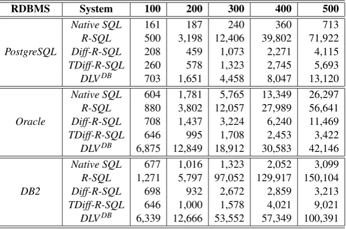
importance of introducing the semi-na¨ıve differential optimization [Ull85]. To make the compar-ison fairest with the RDBMS’s, which do not discard duplicates, we omit the operatorEXCEPT to behave similarly to the optimized R-SQL systems. Also, we include the last published ver-sion ofDLVDB in this comparison as a deductive system which is able to project its solving to these external databases when computing a transitive closure. Another related deductive system is LDL++, but unfortunately it is not included in this comparison since it has been replaced by the system DeALS whose binaries and/or sources are not available yet.
RDBMS System 100 200 300 400 500
Native SQL 161 187 240 360 713
R-SQL 500 3,198 12,406 39,802 71,922 PostgreSQL Diff-R-SQL 208 459 1,073 2,271 4,115 TDiff-R-SQL 260 578 1,323 2,745 5,693 DLVDB 703 1,651 4,458 8,047 13,120 Native SQL 604 1,781 5,765 13,349 26,297 R-SQL 880 3,802 12,057 27,989 56,641 Oracle Diff-R-SQL 708 1,437 3,224 6,240 11,469 TDiff-R-SQL 646 995 1,708 2,453 3,422 DLVDB 6,875 12,849 18,912 30,583 42,146 Native SQL 677 1,016 1,323 2,052 3,099 R-SQL 1,271 5,797 97,052 129,917 150,104 DB2 Diff-R-SQL 698 932 2,672 2,859 3,213 TDiff-R-SQL 646 1,000 1,578 4,021 9,021 DLVDB 6,339 12,666 53,552 57,349 100,391
Table 2: Analysis of Systems
The results for different instances of the benchmark are given in Table2. Numbers are now arranged with the parameternranging in the horizontal axis, and rows include the considered RDBMS (first column), the system connected to this relational database (second column), and then (in the next five columns), the wall time for solving each instance (from 100 up to 500 tuples in the relationflight, which delivers from 5,050 up to 125,250 tuples in the result set of the query benchmark). Below the headings, lines are arranged in major rows, each one referring to a concrete RDBMS. And, for each RDBMS (PostgreSQL,Oracle,DB2)4, five minor rows are listed, which refer to each system. The first minor rowNative SQLrefers to the corresponding RDBMS, which is used to compare how the rest of the systems behave w.r.t. a native execution of the benchmark, i.e., resorting to the recursive query specification for the transitive closure that each RDBMS provides. For instance, DB2 uses the following syntax (where rec is the temporary recursive relation which is built to fill the relationreachable):
INSERT INTO reachable WITH rec(frm,to) AS
(SELECT * FROM flight UNION ALL
SELECT flight.frm, rec.to FROM flight,rec WHERE flight.to = rec.frm)
SELECT * FROM rec;
The next minor rowR-SQLrefers to the implementation we have presented in Section 3. Minor row labeled with Diff-R-SQL presents the results for R-SQL with the semi-na¨ıve differential optimization enabled as explained in [Ull85]. Roughly, for a linear query, this optimization refers to use in each iteration only the results that have been generated in the previous iteration to build new tuples. To implement this, we have resorted to add a new integer column (itin the benchmark) holding the iteration in which a given tuple has been generated. For instance, the next query is executed for each iteration$IT$(this is substituted by the actual iteration number along iterations):
INSERT INTO reachable
SELECT flight.frm, reachable.to, $IT$ FROM flight, reachable
WHERE flight.to = reachable.frm AND reachable.it = $IT$-1;
Next, the row labeled withTDiff-R-SQLrefers to an alternative implementation of the semi-na¨ıve differential optimization, which consists on storing all the tuples generated in a given iteration in a temporary table. Then, the join at each iteration is computed betweenflightand this temporary table, therefore avoiding to scan the growing relationreachablelooking for the tuples with a given iteration number value in the extra field. In fact, two temporary tables are needed: One for accessing the tuples generated in the previous iteration, and another one to store the new tuples. Next, there is a sketch of the SQL statements submitted in each iteration to DB2, wherereachable temp1 is intended to hold the tuples generated in the previous iteration, andreachable temp2is for the current one (temporary tables are preceded bySESSION.):
INSERT INTO SESSION.reachable_temp2
SELECT flight.ori, SESSION.reachable_temp1.des FROM flight, SESSION.reachable_temp1
WHERE flight.des = SESSION.reachable_temp1.ori; ...
INSERT INTO reachable SELECT * FROM SESSION.reachable_temp1; DELETE FROM SESSION.reachable_temp1;
INSERT INTO SESSION.reachable_temp1 SELECT * FROM SESSION.reachable_temp2; DELETE FROM SESSION.reachable_temp2;
The first SQL sentence loads intoreachable temp2the results just computed for the cur-rent iteration. Next sentences simply load onreachablethe results from the previous iteration, and transfer the results just available inreachable temp2toreachable temp1in order for them to be available for the next iteration.reachable temp2is finally flushed to be ready for the next iteration as well.
Finally, the row labeled with DLVDB stands for this deductive system, which uses the same ODBC bridge to access those relational systems.
Looking at the numbers, it is noticeable that the best performance is achieved by the native SQL execution in PostgreSQL for all the considered instances (n∈ {100,200, . . . ,500}) of the benchmark. Also, the worst performance corresponds to R-SQL without optimizations (and including the operatorEXCEPT), which is also clear as the join and the difference must be pro-cessed in each iteration for all the tuples, including those that definitely will not be involved in generating a new one. The semi-na¨ıve differential optimization (which also avoids the operator
EXCEPT) alleviates this enormously, with a huge factor of 150,104/3,213=46.7×, when
com-paringR-SQLvs. Diff-R-SQLfor DB2. DLVDBis the next system in the performance ranking, behaving better than R-SQL but worse than the rest. Depending on the RDBMS, the next best system can be eitherDiff-R-SQLorTDiff-R-SQL: The first one performs better than the second for PostgreSQL and the other way round for Oracle and DB2. Noticeably, both perform better thanNative SQLfor Oracle, and Diff-R-SQLbehaves roughly similar to DB2. These numbers highlight how similar techniques are differently managed by the different RDBMS’s. For ex-ample, whereas for Oracle the use of temporary tables is of paramount importance for lowering the solving time, its effect is the contrary for DB2. We have also tested table functions, which provide a way to implement parametric views. However, they do not provide better performance than the already illustrated optimizations (and Oracle faces the mutating table problem when using them to insert tuples in the same source table).
All in all, in the best case we are able to beat an RDBMS by a factor of 26,297/3,422=
7.7×, and in the worst case (but considering the best optimization) we are beaten by a factor of 4,115/713=5.8×. To better understand this slowdown, we must consider that the R-SQL system runs an interpreted script (Python) and in each iteration, one or several SQL statements are sent to the RDBMS via the ODBC bridge. SQL statements sent in this way must be compiled by the RDBMS for each iteration, so that it becomes a significant burden on the system, together with the communication cost due to the bridge. Therefore, using a compiled language supporting prepared SQL statements should be a point worth to explore for performance gains.
4
Conclusions
R-SQL has been designed to compute the meaning of a database definition and then to query this database. Notice that the modification of a relation of the database in the underlying RDBMS can cause inconsistencies since the tables are not recomputed. For instance, after processing the database for flights, if the user adds or deletes a tuple for the relationflight, then the relation
3.2 to get a lazy evaluation of such relations, performing iterations only when new values are demanded.
As shown in Section3.3.2, the semi-na¨ıve differential optimization [Ull89] for linear recur-sive queries has a notable impact on performance. Nonetheless, our system can be further ex-tended for non linear recursive queries and with enhancements as in [ZCF+97,BR87], as DLV [TLLP08] does. Implementing all these optimizations are left for future work.
Although our proposal is encouraging as results reveal, efficiency can also be improved by indexing (e.g., tries [SW12] and BDD’s [WACL05]) temporary relations during fixpoint compu-tations. To seamlessly integrate this into an RDBMS, we can profit from the fourth-generation languages (e.g., SQL PL in IBM DB2 and PL/SQL in Oracle) and completely integrate query solving and view maintenance into the RDBMS. This way, prepared SQL statements are avail-able in a compiled setting, which should also improve performance. We are currently extending the R-SQL system with the enhancements aforementioned and more features as hypothetical definitions and aggregates.
Bibliography
[ANSS13] G. Aranda-L´opez, S. Nieva, F. S´aenz-P´erez, J. S´anchez-Hern´andez. Formalizing a Broader Recursion Coverage in SQL. In Symposium on Practical Aspects of Declar-ative Languages (PADL’13). LNCS 7752, pp. 93 – 108. 2013.
[AOT+03] F. Arni, K. Ong, S. Tsur, H. Wang, C. Zaniolo. The Deductive Database System LDL++.TPLP3(1):61–94, 2003.
[BR87] I. Balbin, K. Ramamohanarao. A Generalization of the Differential Approach to Recursive Query Evaluation.J. Log. Program.4(3):259–262, 1987.
[Cod70] E. Codd. A Relational Model for Large Shared Databanks.Communications of the ACM13(6):377–390, June 1970.
[Dat09] C. J. Date.SQL and relational theory: how to write accurate SQL code. O’Reilly, Sebastopol, CA, 2009.
[FMMP96] S. J. Finkelstein, N. Mattos, I. S. Mumick, H. Pirahesh. Expressing Recursive Queries in SQL. Technical report, ISO, 1996.
[GUW09] H. Garcia-Molina, J. D. Ullman, J. Widom.Database systems - the complete book (2. ed.). Pearson Education, 2009.
[KRP93] O. Kaser, C. R. Ramakrishnan, S. Pawagi. On the conversion of indirect to direct recursion.ACM Lett. Program. Lang. Syst.2(1-4):151–164, Mar. 1993.
[MP94] I. S. Mumick, H. Pirahesh. Implementation of magic-sets in a relational database system.SIGMOD Rec.23:103–114, May 1994.
[SW12] T. Swift, D. S. Warren. XSB: Extending Prolog with Tabled Logic Programming. TPLP12(1-2):157–187, 2012.
[TLLP08] G. Terracina, N. Leone, V. Lio, C. Panetta. Experimenting with recursive queries in database and logic programming systems.TPLP8(2):129–165, 2008.
[Ull85] J. D. Ullman. Implementation of Logical Query Languages for Databases. ACM Trans. Database Syst.10(3):289–321, 1985.
[Ull89] J. Ullman.Principles of Database and Knowledge-Base Systems Vols. I (Classical Database Systems) and II (The New Technologies). Computer Science Press, 1989.
[WACL05] J. Whaley, D. Avots, M. Carbin, M. S. Lam. Using Datalog with binary decision diagrams for program analysis. InIn Proceedings of Programming Languages and Systems: Third Asian Symposium. 2005.