PROBABILITY DISTRIBUTIONS ASSESSMENT FOR
MODELING GAS CONCENTRATION IN CAMPO GRANDE, MS,
BRAZIL.
Amaury de Souza,
[a]Zaccheus Olaofe,
[b]Shiva Prashanth Kumar Kodicherla,
[c]Priscilla Ikefuti,
[d]Luciana Nobrega
[e]and Ismail Sabbah
[f]Keywords: Statistical analysis; distribution of probability; performance indicators; air pollutants.
The predominant air pollutants in urban cities are (NOx = (NO + NO2), O3 and (OX = (O3 + NO2). This research focused on pollutant
variables that cause damage to human health as well as to the environment. Thus, seven statistical models {Weibull (W), Gamma (G), Log-normal (L), Frechet (Fr), Burr (Bur), Rayleigh (R) and Rician (Ri)} were chosen to fit the observations of the air pollutants. An average hourly data from one year to 2015 were considered. In addition, performance indicators {Mean Absolute Error (MAE), Root Mean Square Error (RMSE), Mean Absolute Percentage Error (MAPE)} were applied, to determine the quality criteria for adjustment of the frequency distributions. The best distribution that adapts to the observations of the variables was the RICIAN distribution, the log-normal distribution for COD. The probabilities of the concentration of exceedances were calculated,(predicted) from the cumulative density function (cdf) obtained from the best fit distributions.
*Corresponding Authors
E-Mail: [email protected]
[a] Federal University of Mato Grosso do Sul, C.P. 549, 79070-900 Campo Grande, MS – Brazil
[b] University of Cape Town: Rondebosch, Western cape, South Africa.
[c] Department of Civil Engineering, Room No. EB 577, Engineering Building (EB), Xi'an Jiaotong-Liverpool University (XJTLU), Suzhou Industrial Park, Suzhou, P. R. China.
[d] University of São Paulo; Department of Physical Geograpy, São Paulo- SP- Brazil
[e] Universidade Federal da Paraiba, Depto de Engenharia dos Materiais, João Pessoa, PB, Brasil
[f] Department of o Natural Sciences, College of Health Sciences, the Public Authority for Applied Education and Training, Kuwait
INTRODUCTION
Air pollution in urban areas causes adverse effects on the human health and the environment. In addition, cities face increasing urban pollution and it has negative effects on the rapid population growth. Recent studies have also proven over time that industrialization and the use of motor vehicles are the two main contributors to urban air pollutions.
One of the main problems caused by air pollution in the urban areas is the presence of photochemical oxidizers. Among these pollutants, ozone (O3) and nitrogen dioxide
(NO2) are particularly important since they are susceptible to
provoking adverse effects on the human health (OMS, 2000). The formation of ozone at ground level depends on the intensity of the solar radiation, the absolute concentration of NOx and the VOCs (Volatile Organic Compounds), and the ratio between NOx and VOCs.1
The ozone concentration increases with the growing intensities of solar radiation and the air temperature. The concentration of photochemical oxidizers may be reduced throughout the control of their precursors, which are nitrogen oxides NOx (NO and NO2) and VOCs.2-8
In Campo Grande, some studies and climate monitoring campaigns have been carried out,2,9-17 for studying the
atmospheric dispersion modelling to explore the results of climate change.
In literature, probability distributions have been used to adjust the concentrations of air pollutants, including the: Weibull distribution,18 Lognormal distribution,19 Gamma
distribution,20 distribution of Rayleigh,21 distribution of
Gumbel22 and Frechet's distribution.23 Using a variety of
performance indicators, such as the: mean absolute error (MAE), root mean square error (RMSE), concordance index (d2), bias normalized absolute error (NAE), prediction accuracy) and the coefficient of determination (R2).
The objectives of this study are to adjust the probability distributions for the concentration of three air pollutants (NOx, O3 and OX) using seven statistical models.
MATERIALS AND METHODS
Studied and observational data
Campo Grande is the capital city of South Mato Grosso (MS) state, located in the southern of Brazil Midwest region, sited in the center of the state. Geographically, the city is near to the Brazilian border with Paraguay and Bolivia. It is located at 20°26’34’’ South and 54°38’47’’ West longitude. Figure 1 shows the location of Campo Grande, capital of the state of Mato Grosso Sul (MS). It occupies a total area of 8,096.051 km² or 3,126 mi², representing 2.26 % of the total state area, within 860,000 inhabitants (2016) and a corresponding HDI of 0.78. The urban area is approximately 154.45 km² or 60 mi², where tropical climate and dry seasons predominate, with two clearly defined seasons:
warm and humid in the summer, and less rainy and mild temperatures in winter months.
During the months of the winter, the temperature can drop considerably, arriving on certain occasions to the thermal
sensation of 0 ºC or 32 ºF with occasional and light freezing. The year average precipitation is usually at 1,534 mm, with
small up or down variations. The main pollution problems in the city are attributed to the: traffic of vehicles, raise of building activities, the presence of dumping grounds, use of small power generators running on oil to supply power to the electric grid, and finally, to the induced fire outbreak
used to clean up local terrains.
Ensemble of observational data
The air quality and meteorological variables are monitored by an automatic station operated at the Institute of Physics of the Federal University of South Mato Grosso (UFMS). This met station is located inside the university campus,
about 8 km or 5 miles to the west of downtown. The main sources of pollution in that area are the building activities; therefore, there are no significant precursor sources of ozone identified close to the region. The ozone levels of Campo Grande area are stored in a regular database since 2004.
The equipment of measurements was installed at the top of a tower from where air samples are extracted throug vertical pipes that are placed approximately 2 meters above the ground level.
The three considered pollutants, NOx (NO + NO2), OX
(O3 + NO2) and O3, were measured continuously for a one–
year period (2015).
The equipment used for measurements include a nitrogen oxide analyzer (AC31M–using chemiluminescence method), an ozone analyzer (O341M–LCD/UV Photometry). All equipment was made by Environnement S.A.
Modelling of the climatological datasets
The statistical models (Weibul, Rayleigh, Gamma, Lognormal, Frechet, Burr and Rician) used for fitting of the observeddatasets (NOx, OX and O3)are defined as follow:
Weibull (W) PDF
The Weibull probability density function (pdf) of a 2-parameter distribution is given as the derivative of a cumulative distribution function (cdf) expressed in Eqn. (1)
(1)
The Weibull cumulative distribution function (cdf) is given by Eqn. (2)
(2)
where
k and C are the shape and scale parameters of the Weibull distributions derived from the time series of the climatological datasets;
is the time series observations from each variable/dataset.
Meanwhile, the shape parameter “k” is obtained from the
maximum likelihood estimator (MLE) as expressed:
(3)
Once the k values are calculated, the scale parameter values are obtained from Eqn. (4)
(4)
where N is the number of time series dataset points. Meanwhile, Eq. (3) is apply to each climate observations and solve iteratively with an initial guess of 2 (k=2) until k
values converge after several iterations.
w
k-1
k
v v
k
(k,C) = exp -C
C C
f
w
k
1
ν
F (k,C) = exp
-C
k i ik
i
-1
N
N
ln
ln( )
νi
i=1
i=1
=
-N
ln
i=1
k
N
1 N k
k i i 1
=
N
Rayleigh (R)P DF
Substituting k=2 into Eqs (1) and (2), the Rayleigh pdf of a continuous distribution fr (v,k,C), is given as:
(5)
The Rayleigh cumulative distribution function (cdf) is given:
(6)
Gamma (G) PDF
The pdf of a gamma distribution is defined by Olaofe and Folly:24
(7)
where fg and Γ(k) are the pdf of gamma distribution and the gamma function of (k), respectively. k and C are the shape and scale parameters of the Gamma distribution derived from the time series observations.
The cumulative density function (cdf) of a Gamma distribution is defined as
(8)
where Fg is the cumulative density function of a gamma
distribution.
Lognormal (L) PDF
Lognormal was used to fit the ozone concentration data. The location parameter of the lognormal distribution is estimated from the expression:
(9)
where is the variance of the observed dataset and μ is the lognormal scale (sigma) parameter
The scale parameter of the lognormal distribution is estimated as
(10)
where is the (location) parameter.
The probability density function and the cumulative distribution function of a lognormal pdf are defined below
(11a)
(11b)
where
, μ,fl, Fl and erfc(ln-)
2/22 are the location
parameter, scale (sigma) parameter, lognormal pdf and cdf, and error function of (ln-)2/22, respectively.
In another literature,25 the lognormal distribution with
probability density function was given by Lu:
(12a)
The cumulative density function form for normal distribution is
(12b)
𝜎 is obtained by solution below
(12c)
and α by using solution below 2 r
2
v
(k,C) =
exp
-C
C
2v
f
2 r1
C
(k,C) = - exp
F
k 1 g k
v (k,C) = exp-Γ(k) C
f
C
2
ln 1
g kk-1
v
1
t
(k,C) =
t
exp -
dt
C Γ(k)
0
C
F
2 2ln
2 l 21
ln(
)
( , )
exp
2
2
f
2 l 2(ln
)
( , ) 1 erfc
2
F
21
1 ln
( )
exp
2
2
x
f x
x
2 ln x x 21
( )
e
d
2
f x
t
n i i 1
1
ln( )
x
(12d)
Frechet (F) PDF
The density function of the generalized extreme value (GEV) distribution with shape (k≠0), location (µ) and the scale (δ) parameters are given:26
(13)
where ff is the probability density function of a Frechet (GEV) distribution
Rician (Ri) PDF
The density function of a Rician distribution is given as:27
(14)
where
s≥0 and δ=0 are non-centrality and scale parameters, respectively;
Ι0 is the zero-order modified Bessel function of the first kind.
The two parameters of the Rician distribution are estimated as:
(15)
(16)
where Ι1(z) is the first-order modified Bessel function of the first kind and z=is/2. A good numerical optimization
algorithm with a starting value is needed to solve Eqn. (15).
Burr (B) PDF
The density function (pdf) of the Burr distribution is given by the expression:
(17)
Accuracy Test
The accuracy results are essential for determining the effectiveness of the statistical models. Thus, accuracy check is carried out by comparing the observed climate distribution with predicted/modeled distributions. The observed data is the values from the monitoring systems whereas the modeled datasets are obtained from the fitted distributions.26 The various tests for determining the
goodness-of-fit of the models (pdfs) are expressed below:
Mean Absolute Error (MAE)
The mean absolute error is used for testing the predicted distribution of observed climatological variables (NOx, OX
and O3) against the observed distribution. It is often defined
as the mean of the absolute errors derived from the observed and predicted values. The mathematical equation is defined as:
(18)
where
xi is the observed values of the air pollutants;
is the predicted/modeled values from Weibull, Rayleigh, and Gamma, Lognormal models etc.
Root Mean Square Error (RMSE)
It is used for comparison of the predicted from the observed values. The root means square error for the best fit statistical model is given as:
(19)
Mean Absolute Percentage Error (MAPE)
The mean absolute percentage error is calculated as:
(20)
RESULTS AND DISCUSSIONS
The description statistics of average values of air pollutants for the sampling period (2015) was being shown in Table 1. The annual mean values of the gases (NO, NO2,
NOx, OX and O3) was higher than the median, indicating a
high concentration recorded for the studied period. Most of the data is concentrated to the left of PDF charts with few high values. There was an increase in mean, median, roughness and persuasion values, indicating a growing problem of air pollution in Campo Grande.
i
1
ln( )
x
n
f 1 1 1 k k( , , )
1
exp
1
1
f k
k
k
2 2n 0 2 2 2
(
)
( , )
exp
2
s
s
f s
I
N 1 i
i 1 0
( )
1
( )
I z
s
N
I z
N 2 2 i i 1
1
0.5
N
s
2 2
bur
( , )
I0
2 2exp
22
s
s
f
s
N i i i 1MAE
y
x
N
1/ 2 N i i i 1RMSE
y
x
N
N i i i 11
MAPE
100
Table 1. Descriptive analysis of pollutants for the sampling period (2015).
Variable Count Mean St.Dev Coef.Var Minimum Median Maximum Skewness Kurtosis
NO (ppb) 8776 7.069 11.583 163.87 0.000 3.700 165.000 5.11 38.11
NO2 (ppb) 8776 5.6624 5.6530 99.84 0.0000 4.1000 60.2000 2.41 9.63
NOx (ppb) 8776 12.721 13.708 107.76 0.000 8.800 165.000 3.39 18.25
OX (ppb) 8776 21.766 10.826 49.74 2.000 20.200 95.400 1.04 2.23
O3 (ppb) 8776 16.109 9.832 61.03 1.000 15.100 79.700 1.00 1.99
Source: UFMS-Institute of Physics
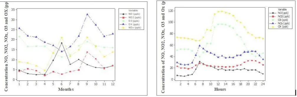
Figure 2. Average of measured values for a daily period of NO, NO2, NOx, O3 and Ox concentrations. The interval between measurements
equals 1 hour.
Hourly variation of O3, NO, NO2, OX and NOx concentrations The average per diem variation observed for the NO, NO2,
NOx, OX and O3 concentrations are presented in Fig 2.
Generally, the daily cycle of the ozone concentration reaches its peak at middle day and presents smaller concentrations during the night. The ozone concentration slowly increases after the first rays of the sunshine, getting to its maximum value during the daylight period, and after which it starts to decrease slowly until the next morning.
Figure 2 shows a displacement of about 2 hours in the morning between the NO and NO2 peaks. In the morning,
NO2 is produced by oxidation of NO,2 because NO can be
converted to NO2 in the presence of peroxy radicals, but at
night, NO and NO2 concentrations have a slight increase
caused by increased in vehicular traffic during the rush hour (6:00 p.m.) and the influence of night boundary layer stability. At this time NO2 reached its peaks at 6:00 p.m.
Figure 2 shows an increase in O3 concentrations during
the day, starting at 8:00 p.m. and peaking at 2 p.m. NO is converted to NO2 by reaction with O3, but during the
daytime, NO2 is converted back to NO as a result of
photolysis, which leads to O3 regeneration.8 O3
concentration in urban atmospheres peaked during the daytime from at 14:00 - 15:00, when there is a maximum in solar radiation intensities and air temperature. This increase is by photolysis of NO2 and by the increase in the height of
the boundary layer during the daytime that can result in the O3 mixture due to thermal stratification and convective heat
transfer to the surface of the air at higher altitudes. After reaching the maximum concentration at 14:00-15:00 hr., the concentration of O3 decreases due to a decrease of the
photochemical activity.
Higher OX concentrations occurred in the afternoon, thus revealing an influence of the photochemical processes.5,8
Also, OX decreases due to the absence of solar radiation at night. This lack of radiation hinders the formation of NO2
and O3 by photolytic reactions, as well as the reactions of
NO2 with NO3, and of NO2 with O3.28
While O3 and a large percentage of NO2 concentrations
are the secondary contaminants, NO is a primary contaminant, formed through a complex set of chemical reactions. At 07:00 a.m, the sunlight begins to induce a series of photochemical reactions. NO is converted in NO2
through a reaction with O3. During the shining hours, NO2
is converted again into NO because of photolysis, which induces the regeneration of O3.
Another factor influencing the atmospheric air pollutant concentrations is the height of the mixture layer over the city. In a shiny day, the pollutants are diluted when the mixture layer increases during the day and stays limited to the inside of NPBL during the night. Emitted pollutants, like NO, are kept underneath (such an inversion), and it can cause an increase of hourly average concentration of NOx
Chemistry of O3, NO and NO2
The basic chemistry that led to the production and destruction of ozone has been detailed elsewhere.28
NO2 + h NO + O (21)
O + O2 O3 + M (22)
O3 + NO NO2 + O2 (23)
M represents a molecule absorbing the excess of vibrational energy and thus stabilizing the O3 molecule that
has been formed, normally it is N2 or O2; h represents the
photon energy, with a 424 nm wavelength; and O is an active monoatomic molecule of oxygen.
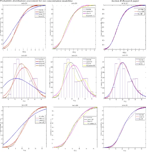
The plots of the pdfs and cdfs for three air pollutant variables (NO, O3, OX) in Campo Grande are presented in
Fig 3. The plots show that for: NO - the functions (W, R, and
G), fit well in the range of 0 to 30 ppb ; For the functions (L,
Ri, NP), they overestimate in the range of 0 to 3, underestimate in the range of 3 to 12 and overestimate in the range of 12 to 30 ppb. The functions that fit the NO concentration best are Rayleigh and Rician. (please confirm again W, R, G, L, Ri, NP. Also, I don't know what NP stands for)
O3- the functions (W, R and G) underestimates the concentrations of 0 to 18 ppb and overestimate in the range of 18 to 35 ppb, while the R function overestimates in the
Figure 3. – Plots of the pdfs and cdfs for three air pollutant variables (NO, O3, OX) in Campo Grande.
OX- for the functions (W, R, G) underestimates the concentrations of 0 to 25 ppb and overestimate in the range of 25 to 40 ppb; For the functions (L, RI, NP) overestimated in the range of 0 to 15 ppb, underestimated in the range of 15 to 28 for Ri and overestimated for L and NP in the range of 15 to 23 ppb, in the range of 28 to 40 overestimate To Ri and underestimated for L and NP. The best function that fits for OX is Rician. In order to compare the quality of several pdfs to sample variable concentration data, several statistics were used in related studies for analysis of O3, NO and OX.
The most used are coefficient of determination, Chi-square (χ2) test results, Kolmogorov-Smirnov test (KS) and square
root mean square error (RMSE). In most studies, a visual evaluation of overlapping adjusted pdfs To the histograms of the data is also performed The RMSE are applied in theoretical cumulative probabilities against empirical or theoretical cumulative probabilities of the concentrations of
the observed variables. These statistics are also calculated with variable data in the form of frequency histograms.
In addition to the analysis performed on the distributions of the variables, some authors also evaluated the adequacy of pdfs to adjust the concentration distributions obtained by the sample variables or to predict the concentrations. In this case, the pdfs are first adjusted to the data of the variables. Then, the theoretical distributions of concentration density are derived from the pdfs adjusted for the variables. Finally, the fit quality measurements are calculated using the theoretical density distributions and the distribution estimated from the NO, O3, OX variables of the sample.
Graphically, it can be seen that the Rician PDF produces the best fit. Rayleigh and gamma distributions correspond to the histogram to a lesser extent and provide the poorest adjustments. It can be seen from the figures that these variables present different forms of histograms. The parameter values obtained for these distributions and the assembly precision based on the performance index criteria presented in Table 2. It can be seen that both statistical indicators gave similar results in all cases. The Weibull (W), Rician (Ri), log-normal (L) functions provide the smallest adjustment error for the data sets. This is also verified in Figure 3. Statistical tests show that the Rician distribution is the best choice for the data set. However, the Weibull PDF also provides fairly accurate results for the variables. Rayleigh PDF gives a very poor performance and is a poor fit. The performance of these three PDFs to evaluate the concentrations of the variables were also analyzed and the results are summarized in Table 2.
The Rayleigh PDF produced the maximum error between the PDFs and produced significant errors in the evaluation of the concentrations of the variables. Overall, Weibull, Rician, and lognormal PDFs resulted in fewer errors, and among the three functions, while Rician was ranked number 1 based on performance index criteria. It can be said that the evaluation of these distribution functions based on the quality of the adjustment criteria alone is not enough. These criteria should be used to identify appropriate distributions before a detailed analysis is made. As these PDFs installed can be used for different applications by the industries, public managers in decision-making, the performance of these PDFs for specific applications, such as prediction of the concentration of pollutants, should also be evaluated. The results show that there are an underestimation and overestimation of the concentration density of the pollutants in general, depending on the concentration range. The percentage errors mainly show that this underestimation and overestimation of the concentrations of these pollutants, which may be due to the heating effect and the atmosphere.
The distributions gamma has also been used to fit the probability density functions of daily air pollutant concentration.29 The pollutants studied have a different
statistical distribution, due to the different diffusion characteristics of the individual pollutant in the air and to the interaction of diffusion characteristics and local geography, climatic conditions in Campo Grande. The distributions gamma has also been used to fit the probability density functions of daily air pollutant concentration.29
The current study showed that the pollutants studied O3,
OX and NO had different statistical distribution. The difference might be due to the different diffusion characteristics of individual pollutant in the air, and the interaction of diffusion characteristics and local geography, weather conditions in Campo Grande. The underlying mechanisms need to be further explored.
The current analysis shows that the statistical distributions of better performance of several air pollutants in Campo
Grande are different. For example, Nan-Hung Hsieh and Chung-Min Liao claimed that the probability distributions for all air pollutants in Taiwan were approximate to be a lognormal distribution.30 In addition, Neustadter31 revealed
that the total suspended particulate is obviously logically distributed, whereas sulfur dioxide and nitrogen dioxide are rationally estimated by lognormal distributions. However, Oguntunde32 showed that the Gamma pdf is the best
distribution model for the carbon monoxide concentration modelling in Lagos State, Nigeria. Hai-Dong Kan and Bing-Heng Chen indicated that the best fit distributions for PM10 concentrations in Shanghai were lognormal.33
In Malaysia, Noor et al.26 found that the best distribution
fits the PM10 observations in Nilai was the Gamma distribution while the log-normal distribution is more appropriate in Shah Alam. Razali et al. referred to lognormal distribution as the best distribution that fitted to the carbon monoxide data in Bangi, Malaysia.34 Accordingly, there is
no common distribution of air pollutants and it differs from the studied region and time. It is important to carry out a comparative analysis in order to find out which distribution better fits the air pollutants in a particular location in order to provide a better estimate of the air quality at that location.
Table 2 presents the results tests for fitting for different distributions to the air pollutants data. The preferable results were highlighted by italicizing and bold. We found that out of the distributions considered, the Rician and Gamma distribution significantly fits with most of the air pollutants data in Campo Grande which are NO, O3 and OX, while O3
is fitted well with Weibull distribution.
Performance Indicators
The values of the performance indicators for the variables concentration in Campo Grande were tabulated in Table 2. A small value of the MAE indicates that the distribution of the Rician fits well the sampled data of the variables (O3 and
OX), while the best fit that is appropriated is the function of Rayleigh. The smaller MSE and RMSE values indicate that the physician's distribution best fits the variables data while the lower COD value indicates that the Rician distribution fits the variable data
CONCLUSION
Based on the statistical characteristics of the concentrated air variables studied in Campo Grande, result findings indicate that the mean of the concentrations of the variables for the monitoring data sets was higher than the values of the medians showing that all observations are positively inclined to the right, with few extreme concentrations. The Weibull (W), gamma (G), log-normal (L), Frechet (Fr), Burr (Bur), Rayleigh (R) and Rician (Ri) distributions have been analyzed with the selected datasets.
MAE
Datasets Weib Rayl Gam Logn Rician Frechet Burr
NO 0.0121 0.0100 0.0185 0.0665 0.0118 0.0224 0.0217
O3 0.0025 0.0167 0.0088 0.0422 0.0015 0.0237 0.0083
OX 0.0024 0.0152 0.0057 0.0437 0.0003 0.0247 0.0275
MSE
Datasets Weib Rayl Gam Logn Rician Frechet Burr
NO 0.00021 0.00014 0.00048 0.000997 0.0001422 0.00069 0.00064
O3 0.00001 0.00040 0.00010 0.00023 0.0000031 0.00079 0.00011
OX 0.00001 0.00033 0.00004 9.49E-05 0.0000001 0.00094 0.00108
RMSE
Datasets Weib Rayl Gam Logn Rician Frechet Burr
NO 0.0143 0.0119 0.0220 0.031571 0.0119 0.0263 0.0252
O3 0.0029 0.0201 0.0101 0.015156 0.0018 0.0281 0.0107
OX 0.0028 0.0182 0.0065 0.009742 0.00032 0.0306 0.0328
COD
Datasets Weib Rayl Gam Logn Rician Frechet Burr
NO 0.8662 0.9305 0.8117 0.658254 0.9306 0.8046 0.8278
O3 0.9854 0.4589 0.9173 0.847021 0.9945 0.7032 0.8540
OX 0.9958 0.6093 0.9465 0.890939 0.9998 0.2916 -0.1592
MAPE
Datasets Weib Rayl Gam Logn Rician Frechet Burr
NO 6.6708 8.0654 6.7749 -3.2820 8.0636 4.8187 5.7405
O3 3.1229 -67.4508 4.5800 -45.0314 1.6711 -22.5415 -1.2100
OX -0.5213 -37.8984 1.7815 -1.6104 0.3108 -32.7144 82.4431
Performance indicators were also applied, which were
mean absolute error (MAE), root mean square error (RMSE), the mean absolute percentage error (MAPE) to determine the quality criteria for the adjustment of the distributions.
The best distribution that adapts to the observations of the variables was the Rician, Weibull and the lognormal distribution. The pdf and cdf graphs obtained in this research can be used to predict the probabilities of exceedances.
The importance of statistical analysis in the field of atmospheric pollution for environmental engineering is shown in this research as it’s useful for to adjustment of the data sets of pollutants with the best statistical model, in turn, to successfully estimate the exceedances of pollutants.
However, this work can still be improved with the application of other types of distributions and to adjust the monitoring data of the time series of air pollution.
REFERENCES
1Nevers, N. D., Air Pollution Control Engineering, 2nd ed.
McGraw-Hill Companies, Inc., New York, 2000, 571–573.
2deSouza, A., Aristone, F., Kumar, U., Kovač-Andrić, E., Arsić,
M., Ikefuti, P. and Sabbah, I. Analysis of the Correlations Between NO, NO2 and O3 Concentrations in Campo Grande
– Ms, Brazil., Eur. Chem. Bull., 2017, 6(7), 284-291.
DOI:10.17628/ecb.2017.6.284-291
3Agudelo-Castaeda, D. M., Teixeira, E. C., Rolim, S. B. A.,
Pereira, F. N., & Wiegand, F. Measurement of particle number and related pollutant concentrations in an urban area in South Brazil. Atm. Environ., 2013, 70, 254-262.
https://doi.org/10.1016/j.atmosenv.2013.01.029
4Kurtenbach, R., Kleffmann, J., Niedojadlo, A., Wiesen, P.,
Primary NO2 emissions and their impact on air quality in
traffic environments in Germany. Env. Sci. Eur., 2012, 24, 21. https://doi.org/10.1186/2190-4715-24-21
5Notario, A., Bravo, I., Adame, J. A., Diaz–de–Mera, Y., Aranda,
A., Rodriguez, A., Rodriguez, D., Analysis of NO, NO2,
NOx, O3 and oxidant (OX=O3+NO2) levels measured in a
metropolitan area in the southwest of Iberian Peninsula. Atm.
Res., 2012, 104, 217–226.
6Mazzeo, N. A., Venegas, L. E. and Choren, H. Analysis of NO,
NO2, O3 and NOx Concentrations Measured at a Green Area
of Buenos Aires City during Wintertime. Atm. Environ., 2005, 39, 3055–3068.
https://doi.org/10.1016/j.atmosenv.2005.01.029
7Ghazali N. A, Yahaya A. S., Nasir, M. Y. and Mokhtar M. I. Z.,
Predicting Ozone Concentrations Levels Using Probability Distributions. ARPN Journal of Engineering and Applied Sciences. vol. 9, N. 11 november, 2014.
8de Souza, A.; Kovač, E., Matasovi, B., Markovi, B., Assessment
of Ozone Variations and Meteorological Influences in West Center of Brazil, from 2004 to 2010. Water, Air and Soil Pollution, 2016, 227, 313.; Han, S.; Bian, H., Feng, Y., Liu, A., Li, X., Zeng, F., Zhang, X., Analysis of the Relationship between O3, NO and NO2 in Tianjin, China. Aerosol Air
Qual. Res.,2011, 11, 128–139.
https://doi.org/10.4209/aaqr.2010.07.0055
9deSouza, A., Aristone, F., Arsic, M., Kumar, U., Souza, A.,
Evaluation of Variations in Ground-Level Ozone (O3)
Concentrations. Ozone-Sci. Eng.,2017, 39, in press.
10de Souza, A.; Aristone, F.; Pavao, H. G., Santos, D. A. S., Kovač,
E. Pires, J. C.; Ikefuti, P., Meteorological Impact Factors on the Modeling of Ozone Concentrations Using Analysis of Temporal Series and Multivariate Statistic Methods. Holos (Natal. Online), 2017, 5, 2-16.
11de Souza, A., Kovač, E., Matasovi, B., Markovi, B., Assessment
of Ozone Variations and Meteorological Influences in West Center of Brazil, from 2004 to 2010. Water, Air Soil Pollut., 2016, 227, 313. https://doi.org/10.1007/s11270-016-3002-0 12deSouza, A., Aristone, F., Sabbah, I., Modeling the Surface
Ozone Concentration in Campo Grande (MS)-Brazil Using Neural Networks. Natural Science, 2015, 7, 171-178.
https://doi.org/10.4236/ns.2015.74020
13de Souza, A., Aristone, F., Modeling of Surface and Weather
Effects Ozone Concentration Using Neural Networks in West Center of Brazil. J. Climatol. Weather Forecast., 2015, 3, 1-4-4.
14de Souza, A., Aristone, F., Pavão, H. G., Fernandes, W. A.,
Development of a Short-Term Ozone Prediction Tool in Campo Grande-MS-Brazil Area Based on Meteorological Variables. Open J. Air Pollut., 2014, 3, 42-51.
https://doi.org/10.4236/ojap.2014.32005
15de Souza, A., Aristone, F., Silva, G. B. M., Fernandes, W. A.,
Temporal Variation of the Concentration of Carbon Monoxide in the Center West of Brazil. Atm. Climate Sci.,
2014, 4, 563-568, https://doi.org/10.4236/acs.2014.44051 16de Souza, A., Fernandes, W. A., Surface ozone measurements
and meteorological influences in the urban atmosphere of Campo Grande. Acta Sci. Technol., 2013, 36, 141-146.
https://doi.org/10.4025/actascitechnol.v36i1.18379
17Pires, J. C. M., Souza, A., Pavão, H. G., Martins, F. G., Variation
of surface ozone in Campo Grande, Brazil: meteorological effect analysis and prediction. Environ. Sci. Pollut. Res. Int.,
2014, 21, 10550-10559. https://doi.org/10.1007/s11356-014-2977-6
18Wang, X. and Mauzerall, D. L., Characterizing Distributions of
Surface Ozone and its Impact on Grain Production in China, Japan and South Korea: 1990 and 2020, Atm. Environ., 2004,
38(74), 4383-4402.
https://doi.org/10.1016/j.atmosenv.2004.03.067
19Hadley, A. and Toumi, R. Assessing Changes to the Probability
Distribution of Sulphur Dioxide in the UK Using Lognormal Model. Atm. Environ., 2002, 37(24), 455-467.
20Singh, P., Simultaneous Confidence Intervals for the Successive
Ratios of Scale Parameters, J. Stat. Plan. Infer.,2004, 36(3),
1007-1019.
21Celik, A. N., A Statistical Analysis of Wind Power Density
Based on The Weibull and Rayleigh Models at The Southern Region of Turkey. Renew. Energy, 2003, 29, 593-604.
https://doi.org/10.1016/j.renene.2003.07.002
22Phien, H. N., A Computer Assisted Learning Package for Flood
Frequency Analysis With the Gumbel Distribution, Adv. Eng. Software, 1989, 11, 206-212.
https://doi.org/10.1016/0141-1195(89)90051-X
23Caleyo, F., Velázquez, J. C. Valor, A. and Hallen, J. M.
Probability distribution of pitting corrosion depth and rate in underground pipelines: A Monte Carlo study. Corr. Sci.,
2009, 51, 1925-1934.
https://doi.org/10.1016/j.corsci.2009.05.019
24Olaofe, Z. O. and Folly, K. A., Statistical analysis of wind
resources at Darling for energy production; International J. Renew. Energy Res., 2012, 2(2), 250-251.
25Lu, H. C. Estimating the Emission source reduction of PM10 in
central Taiwan, Chemosphere, 2003, 54, 805-814.
https://doi.org/10.1016/j.chemosphere.2003.10.012
26Noor, N. M., Tan, C. Y., Ramli, N. A., Yahaya, A. S., Yusof, N.
F. F. M., Assessment of various probability distributions to model Pm 10 concentration for industrialized area in peninsula Malaysia: A case study in Shah Alam and Nilai.
Aust. J. Basic Appl. Sci., 2011, 5(12), 2796-2811.
27Olaofe Z. O., Assessment of the offshore wind speed
distributions at selected stations in the South-West Coast, Nigeria; Int. J. Renew. Energy Res., 2017, 7(2), 565-577.
28Jenkin, M. E. and Clemitshaw, K. C., Ozone and other secondary
photochemical pollutants: chemical processes governing their formation in the planetary boundary layer, Atm. Environ.,
2000, 34, 2499–2527, https://doi.org/10.1016/S1352-2310(99)00478-1
29Rumburg, B., Alldredge, R. and Claiborn, C. Statistical
distributions of particulate matter and the error associated with sampling frequency. Atm. Environ., 2001, 35, 2907-2920. https://doi.org/10.1016/S1352-2310(00)00554-9 30Kan, H. D. and Chen, B. H., Statistical Distributions of Ambient
Air Pollutants in Shanghai, China, Biomed., Environ. Sci., 2004, 17, 366-372.
31Neustadter, H. E., Sidik, S. M. and Burr, J. C. Jr., "Statistical
Summary and Trend Evaluation of Air Quality Data for Cleveland, Ohio, in 1967-1971: Total Suspended Particulate, Nitrogen Dioxide, and Sulphur Dioxide," NASA TN D-6935, 1972.
32Oguntunde, P., Odetunmibi O. and Adejumo A., A Study of
Probability Models in Monitoring Environmental Pollution in Nigeria, J. Probability Statistics; 2014, Article ID 864965, 6 pages, http://dx.doi.org/10.1155/2014/864965.
33Hsieh N.-H. and Liao, C.-M., Fluctuations in air pollution give
risk warning signals of asthma hospitalization. Atm. Environ., 2013, 75, 206-216.
https://doi.org/10.1016/j.atmosenv.2013.04.043
34Razali, A. M., Desvina, A. P. Sapuan, M. S. Zaharim, A.,
Distributional Fit of Carbon Monoxide Data. Advances in Environment, Computational Chemistry and Bioscience,
2012, 147-152, ISBN: 978-1-61804-147-0