A Study of Super Nonlinear Motion of Electrostatically Coupled Two Particle System

A Study of Super Nonlinear Motion of

Electrostatically Coupled Two-Particle System

Haiduke Sarafian

University College, The Pennsylvania State University, York, USA. Email: [email protected]

Received July 23rd_{, 2010; revised September 28}th_{, 2010; accepted October 5}th_{, 2010.}

ABSTRACT

We consider a pair of nonidentical mechanical pendulums. The bob of each pendulum in addition to its own mass elec-trically is charged. The pendulums are hung from a common pivot in a vertical plane forming a slanted asymmetric shaped figure. For arbitrary initial swings that are not necessarily confined to small angles, we analyze the dynamics of each bob under the influence of gravity’s pull as well as the mutual repulsive Coulombian internal force. The equa-tions describing the motion of the system are a set of highly, supper nonlinear coupled differential equaequa-tions. Applying Mathematica we solve the equations numerically. For nonidentical parameters describing the pendulums, namely,

0

{ , , , }m q we show the system behaves chaotically; i.e. the angular position of each pendulum leaves a non-repeat-able, chaotic pattern in time. For this coupled two-particle interactive system we show also by folding the time axis, the angular position of one of the pendulums vs. the other traces a Lissajous type curve. Our report includes various tradi-tional phase diagrams and a set of newly designed, useful, phase-type diagrams as well. For a comprehensive under-standing about the dynamics of the problem at hand, we provide Mathematica codes conducive to animating the chaotic motion of the system. The generic format of the codes allows adjusting the relevant parameters at will and addressing the “what-if” scenarios.

Keywords: Nonlinear Motion, Electrostatic Interaction, Deterministic Chaotic Motion, Mathematica

1. Introduction

In search of realistic, practical, nonlinear physics phe-nomena in our previous work we envision a coupled two-particle system [1,2]. In short, we consider a system composed of a pair of mechanical, electrically charged pendulums with a common pivot allowing oscillations in a vertical plane. The design of the system allows an adaptive investigation of the nonlinear oscillations. The mutual electrostatic interaction of the charged pendulums, irrespective the oscillation amplitudes make the oscilla-tions nonlinear by itself. To make the analysis somewhat general, we consider large amplitude oscillations result-ing from gravity pull and electrostatic interaction; appro-priately we called the system “super nonlinear oscilla-tions”. For sake of transparency, however, we assume identical pendulums. Meaning, we assign the same pa-rameters to each pendulum, such as {ℓ,m,q}. Further-more, we apply the same initial conditions such as the initial swing angles and velocities, { , }0 v



to both pen-dulums. Under these conditions, intuitively, it is plausi-ble to conclude the pendulums are to oscillate coherently.

And each pendulum is to trace a repeatable trajectory in time. And indeed we were able quantitatively confirm our intuitive predictions.

To generalize the analysis, in our current work we re-lax the aforementioned restrictions; we consider two non-identical pendulums. We also select nonnon-identical initial conditions. Under these conditions, softly speaking, our intuition is not strong enough to predict and envision the motion of the individual pendulum.

char-acteristic parameters and initial conditions we analyze the problem numerically; we showcase the results. To get a feel for the chaotic motion utilizing Mathematica ani-mation we bring the chaotic motion of the system alive. We also display a few traditional phase diagrams. More-over, we introduce a set of fresh, useful phase-type plots as well. We conclude the paper with a few closing re-marks.

2 2

(F_net) _y m y₂. Here over-dots indicate the second order derivative with respect to time. The x-axis equation yields,

..

2sin 2 12cos 2

T  F  m

   x₂ (1) Here the mutual electrostatic Coulomb force that par-ticle 1 exerts on 2 is ₁₂

2 12

F r



 , where = k q1 q2 with k =

1/(4 ₀) = 8.85 10-12 _{in MKS units; noting the}

dimen-sion of is [] = M L3 _T-2_{. The auxiliary angle shown in}

Figure 1 is subject to cos = (x1-x2)/r12. The abscissa of

the Cartesian coordinate of the second mass can be sub-stituted in terms of the respective angular positions; util-izing Figure 1,

2. Analysis

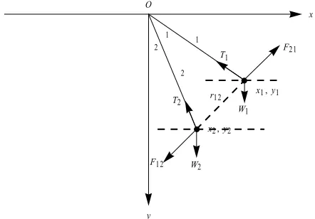
Figure 1 shows the system of interest. It is composed of two asymmetric pendulums. Geometrical, mechanical, and electrical properties of each pendulum is given by the respective set of parameters, namely, { , , , }i m qi i i , with i = 1,2. The θi is the angular position of ith pendulum

from the common vertical reference. The pendulums have a common pivot and are allowed to swing in the vertical plane under the influence of the gravity and their mutual repulsive electrostatic force. The weight, tension and the electrostatic forces are designated by {wi,Ti,Fij}, for i,j =

1,2, respectively.

1 2 1 1 2 2

{ , } { sin ,x x     sin }

cos

. Therefore, in terms of the polar coordinates, cosφ and x-component acceleration of the second particle reads, 1/r12

We consider a case where the movement of the pen-dulums is confined to a 2-dimansional space. Figure 1 displays a snapshot scenario where each pendulum has assumed an angular position θi with respect the vertical

reference. The relevant mechanical forces, namely weight and tension are depicted. We also assume the point-like particles are positively (negatively) charged, so that the mutual electrostatic force as shown is repulsive. We swing the pendulums to arbitrary initial positions to within the lower half plane and release them freely. It is the goal of our study to investigate the consequent mo-tion of each bob.

We begin with Newton’s law of motion, namely,

net

F ma. Applying this equation to the 2nd _particle

along the x and y axis yields, (Fnet)2x m x2 ..2



and

x

y O

　

1

2

　1

W1

W2

　

x1 ,y1

　

x2 ,y2

　

F12

F21

T2

T1

　 　₂

[image:2.595.58.279.538.692.2]

r12

Figure 1. Display of a coupled two-particle system and their relevant mechanical and electrostatic forces.

1 1 2 2

( sin   sin ) and 2 2 2( cos2 2 2 sin )2

x      

  .

Substituting these quantities in Equation (1) and rearrang- ing the terms yields,

1 2

2 2 3 1 2

1 12

. ..

3 2

2

2 12 2 2 2 2

1

sin [ (sin sin )

( cos sin )

T

r

m r

   

   

  



 

 





2

(2)

2 2

(Fnet) ym y 



sin m

, this gives, Similarly we utilize

2cos 2 12 2 2

T  F  g m y2

     (3) Following the steps similar the ones outlined in the previous paragraph, utilizing Figure 1, we write,

1 2 1 1 2 2

{ , } { cos ,y y     cos } . These yields,sin 1/r₁₂

2 2 1 1

( cos   cos ) andy 2

2 2 cos )2 2  2( sin2    

 .

Substituting these in Equation (3) and rearranging the terms gives,

1 2

2 2 3 2 1

1 12

3 2 2

2 12 2 2 2 2

1 1

cos [ ( cos cos )

[ ( sin cos )

T

r g m r

   

   

  

 

 



 _{ }

 

(4)

1 1 1 1 1 1

{ , } { sin , cos }x y      { , }x y_{2 2} 

and because and

2 2

{ sin ,  2cos }2 the distance between the particles

i.e. r12 conveniently can be written in terms of the

rele-vant angular position angles, 2 2

1 2

(y y

 

12 ( 1 2) )

r  x x

2 2

1 2 2 1 2cos( 1 2)

       Now we divide

Equa-tion (2) by EquaEqua-tion (4). After some tedious, laborious algebraic manipulations we arrive at,

.. ..

1 1 2

2 _{2 3 3}

2 2 2 2 1 2 1 2

1 2

2 2

sin( )

sin ( )

[1 ( ) 2 cos( )]

0

g

m

  

 

  

 

  





    

 

The author based on his own experience is convinced manipulating the ratio Equation (2)/Equation(4) yielding Equation (5) is more efficient manually, rather than de-ploying Mathematica symbolic manipulating utilities!

Now we apply F_net mafor particle 1. Following the steps similar to what we have already exercised for parti-cle 2 we derive the equation describing the motion of par- ticle 1,

..

2 1 2

1 _{1 3}

1 1 1 1 2 2 2 2

1 2

1 1

sin( )

sin ( )

[1 ( ) 2 cos( )]

0

3

g

m

  

 

  

 

  





    

 

(6) The set of Equations (5) and (6) are to describe the motion of the coupled two-particle system. Each equa-tion of the set is a second order, homogeneous and highly, super nonlinear ODEs. More over, these equations are coupled via a nonlinear, uneven trigonometry function, if [sin(1 – 2), ℓ1, ℓ2, cos(1 – 2)]. Before we attempt

solving these equations, we make a few observations. First, it is assuring to realize the lengthy algebraic ma-nipulations of the equations yielding Equations (5,6) have the correct features. Meaning, Equation (5) yields Equation (6) for identical pendulums; i.e. for₁₂, m1

= m2 and 01 02. This means under these

assump-tions, the description of the motion of the system is given by only one equation instead of two. Moreover, this one equation is the equation we derived to describing the motion of the symmetrical pendulums in our previous work [1,2]. Second, as we discussed, the non-linearity of the motion has mechanical and electrical origins; these nonlinearities are distinctively separated in Equations (5,6). More specifically, the second and the third coeffi-cients of Equations (5,6) are the strengths of the me-chanical and electrical nonlinear terms, respectively. The coefficient of the electric nonlinear term is composed of two distinct elements; and the rest of the parameters. The value of  as we defined previously is = k q1 q2. Its

value depends on the product of the charges. Assigning different charges to individual particle changes the over-all value of the , however,  contributes evenly to both equations. This is not true for the rest of the charge inde-pendent parameters. Meaning, different values of lengths and masses do contribute unevenly. Therefore, the over-all value of the coefficient of the electric nonlinear term is different in Equations (5,6). Third, since the electro-static interaction is the cause of the coupling one expects by stripping the charge(s) the equations describing the motion should reduce the one describing the oscillations of a mechanical nonlinear pendulum. For this scenario we set = 0; Equations (5,6) yield .. _{sin 0}

i i

i g 

 

  , for

i = 1,2. The latter for small angle approximation i.e. for a

linear oscillator yields the classic linearized equation of motion of a simple pendulum, ..i _{i ~ 0}

i

g

  

 , for i = 1,2.

Now that we have confidence in the correctness of the format of the derived equations, we step forward at-tempting solving them. Because the equations include generic parameters describing the individual pendulum, we have the option of assigning a wide range of parame-ters to characterize each pendulum. For instance, one may consider two pendulums with two different lengths but the same parameters otherwise. Since the third coef-ficient of Equations (5,6) depends on the ratio of the lengths of the pendulums, then for instance in one sce-nario one may study the subsequent impact of assigning rational or irrational and real values to the ratio. Practic-ing one such option would open the “Pandora box”. Ana-lyzing the impact of one such scenario maybe addressed in another research project. For time being in the follow-ing section we study a subset of such options showcasfollow-ing our findings.

3. Numerical Analysis

In the previous section we applied fundamentals of phy- sics principles and developed a set of equations describ-ing the motion of the system. These equations of motion are given with a set of coupled homogeneous highly, super nonlinear ODEs, namely Equations (5,6). To pin point the angular position of each bob at a given time t, one needs to solve these equations expressing angular positions as explicit functions of time, namely {1(t), 2(t)}. In our first attempt to solving these equations we apply various standard symbolic methods. The super non-linearity of the equations come about from the elec-trostatic coupling term, the third terms of Equations (5,6). These are complicated trigonometric two variable func-tions. No wonder we fail solving these equations sym-bolically. We then apply Mathematica DSolve command; it is also unable producing any output. As a last resource we pursue solving these equations numerically. We begin with selecting a set of physically reasonable parameters describing the pendulums, such as {l,m,q}. Then we set the initial conditions, i.e. the initial swing angles of the pendulums. With these parameters on hand, we apply Mathematica NDSolve; it solves the equations. Accord-ing to the aforementioned description the code reads:

In MKS units the pendulums are characterized by, values = {ℓ11.0, m18.*10-3_{, m28.*10}-3_{,q1 1.*}

1.*10-6_{,q21.* 10}-6_{,k9 *10}9_,g9.8};

In this example the pendulums are nonidentical; their initial swing angles are different. One is set at /4and the other one is at 1.2 /4.

The coefficients of the second and the third terms of Equations (5,6) contain the mechanical and the electro-static coupling parameters and are defined by {a’s,b’s}; {a1,b1} for the first and {a2,b2} for the second pendu-lum.

{{a1,b1},{a2,b2}}={{g/ℓ1,(k q1 q2)/(m1 ℓ13_)},

{g/ℓ2,(k q1 q2)/(m2 ℓ23_)}}/.values;

The denominators of the third terms in Equations (5) and (6) are noted by 21 and 12, respectively. Noting, 21=12/.{ℓ1ℓ2, ℓ2ℓ1}

21=(1+(ℓ2/ℓ1)2_{-2 ℓ2/ℓ1Cos[1[t]-2[t]])/.values;}

12=(1+(ℓ1/ℓ2)2_{-2 ℓ1/ℓ2Cos[1[t]-2[t]])/.values;}

We form the ODE’s given by Equations (5,6), these are, eqn1=1''[t]+a1Sin[1[t]]-b1ℓ2/ℓ1Sin[1[t]-2[t]]/

3 2 21

 /.values;

eqn2=2''[t]+a2Sin[2[t]]+b2ℓ1/ℓ2Sin[1[t]-2[t]]/

3 2 12

 /.values;

Utilizing NDSolve we assume symmetrical initial con- ditions and drop the pendulums freely, evenly about the vertical reference through the common pivot. When in-voking NDSolve, we imply the option MaxSteps  otherwise for most of the cases of interest the default numeric solution routine search stops after 1000 itera-tions without searching the desired time span.

soleqns=NDSolve[{eqn1 0,eqn2 0,1[1x 10-8_{] 1init,1'[1*10}-8_{] 0,2[1*10}-8_{] 2init,2'[1*}

10-8_{] 0},{1[t],2[t]},{t,1*10}-8_{,tmax},MaxSteps];}

Utilizing the suppressed output of the numeric solu-tions we evaluate the kinematic quantities of interest such as, position, speed and acceleration of the individual pen- dulum. These set are characterized by Kin1 and kin2.

kin1={position1,speed1,acc1}=Table[D[1[t]/.so leqns1]],{t,n}],{n,0,2}];

kin2={position2,speed2,acc2}=Table[D[2[t]/.so leqns1]],{t,n}],{n,0,2}];

The next couple of lines are used to animate the mo-tion of the swinging pendulums.

x1y1:={ℓ1Sin[1[t]/.soleqns1]]/.values,-ℓ1 os[1[t]/.soleqns1]]/.values}

x2y2:={ℓ2Sin[2[t]/.soleqns1]]/.values,-ℓ2 Cos[2[t]/.soleqns1]]/.values}

tabx1y1=Table[x1y1,{t,0,tmax,0.05}]; tabx2y2=Table[x2y2,{t,0,tmax,0.05}];

Applying Manipulate we display an alive movement of the pendulums. This helps to gain a visual understanding about how the proposed system behaves for the chosen set of parameters. The display panel includes also addi-tional helpful diagrams such as the time series of the an-gular positions of the pendulums, phase profile of the pen- dulums, and the parametric plot of the angular position of

one of the pendulums vs. the other.

Manipu-late[{{Show[Graphics[{Line[{{-2,0},{2.0,0}}],Line[{{0 ,-2},{0,2.5}}],{Hue[0.7],Line[{{0,0},tabx1y1n]}]},{P ointSize[0.025],Hue[0.0],Point[tabx1y1n]]},

{Hue[0.],Line[{{0,0},tabx2y2n]}]},{PointSize[0.025], Hue[0.],Point[tabx2y2n]]}}],ImageSize250,PlotRan ge{{-2,2},{-2,1}}],Plot[{180/Evalate[1[t]/.soleqns 1]],180/Evaluate[2[t]/.soleqns1]]},{t,1

10-8_{,tmax-10.},AxesLabel{"t,s","1,2"},PlotStyle{}

Blue,Red}]},{ParametricPlot[Flaten[{kin21]],kin2 2]]}],{t,1*10-8_{,tmax-50},AxesLabel{" ","}

2

 2"},Aspe

ctRatio1,PlotRangeAll,PlotStyleRed],

ParametricPlot[Flatten[{kin11]],kin12]]}],{t,1* 10-8_{,tmax-50.},AxesLabel{" ","}

1

 ₁"},AspectRatio 1,PlotRangeAll,PlotStyleBlue],

ParametricPlot[Flatten[{kin11]],kin21]]}],{t,1* 10-8_{,tmax-50},AxesLabel{"1","2"},AspectRatio1,}

PlotRangeAll,PlotStyleBlack] }

},{{n,1,"frame"}, 1,Length[tabx1y1],1}]

To show the impact of the initial conditions on the be-havior of the system, in Figure 4 we display plots similar the one shown in Figure 3. The only difference parame-terizing the system is the initial swing angle of the left side pendulum; it is set at02 1.2 / 4 . For instance

the phase profile of the first pendulum displaced by the first graphs of the Figures 3,4 are quite distinguishable. Also the difference between the left lower graphs, the parametric plots of the angular position of the second pendulum vs. the first one is drastic. These very much resemble the Lissajous curves.

Note, a classic Lissajous curve is referred to a closed curve that is being traced by one particle subject to si-multaneous harmonic motions in two perpendicular di-rections. In our study the Lissajous curves are traced by combining the oscillations of two particles subject to oscillations with a relative arbitrary phase difference.

frame

　　

,

20 40 60 80 t,s

　100

　50 50 100

　1,　2

　

,

　

　1.5 　1.0 　0.5 0.5 　2

　4

　2 2 4

　　2

,

　0.5 0.5 1.0 1.5 　1

　4

　2 2 4

　　1

, 　0.5 0.5 1.0 1.5

[image:5.595.57.289.84.257.2]

1 　1.5 　1.0 　0.5 0.5 　2

　　

Figure 2. Top row from left to right: a snapshot of the ani-mation, the time series of the pendulums. Second row: the phase profile of the left (Red) and the right (Blue) pendu-lums, the parametric plot of the angular positions of the second pendulum vs. the first.

　0.5 0.5 1.0 1.5 　1

　4 　2 2 4 　　1

　0.5 0.5 1.0 1.5 　1 　10 10 20 30 40 50 　 .. 1

　4 　2 2 4 　1 　10 10 20 30 40 50 　 .. 1

　0.5 0.5 1.0 1.5 　1

　1.5

　1.0

　0.5 0.5

　2

　4 　2 2 4 　

　₁

　4

　2 2 4

　　2

[image:5.595.316.532.84.218.2]

　10 10 20 30 40 50　 .. 1 　50 　40 　30 　20 　10 10　 .. 2

Figure 3. An extended graphic version of the plots of Figure 2. The second and third plots of the first and the second row are fresh additions to our classic/traditional plots.

0.2 0.4 0.6 0.8 1.0 1.2 　1

　3 　2 　1 1 2 3

　　1

0.2 0.4 0.6 0.8 1.0 1.2　1 10 20 30 40 50 　 .. 1

　3　2　1 1 2 3 　1 10 20 30 40 50 　 .. 1

0.2 0.4 0.6 0.8 1

2 1 1 2 　1

0.2 0.4 0.6 0.8 　1 10 20 30 　 .. 1

　2 　1 1 2 　1 10 20 30 　 .. 1

0.2 0.4 0.6 0.8 1 1.0 0.8 0.6 0.4 0.2 2

2 1 1 2 　

　 1 3 2 1 1 2 3 　2

10 20 30 　 .. 1 　50 　40 　30 　20 　10 10　 .. 2

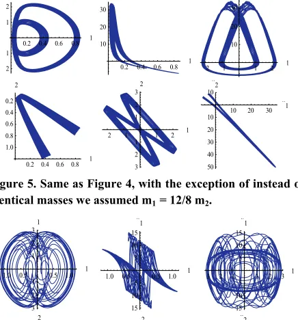
Figure 5. Same as Figure 4, with the exception of instead of identical masses we assumed m1= 12/8 m2.

1.0 0.5 0.5 1.0 1

3 2 1 1 2 3　1

1.0 0.5 0.5 1.0 　1

15 10 5 5 10 15 　 .. 1

　3　2　1 1 2 3　1

　15 　10 　5 5 10 15 　 .. 1

1.0 0.5 0.5 1.0 1

1.0 0.5 0.5 1.0 2

3 2 1 1 2 3　

　 1 2 1 1 2 　2

[image:5.595.316.534.95.329.2]

　15　10　5 5 10 15　 .. 1 　10 　5 5 10 　 .. 2

Figure 6. Same as Figure 4, with the exception of the length of the left side pendulum is21.21.

1.0 0.5 0.5 1.0 1

3 2 1 1 2 3 　1

1.0 0.5 0.5 1.0　1 5

5 　

..

1

　3　2 　1 1 2 3　1 　5

5 　

..

1

1.0 0.5 0.5 1.0 1

1.0 0.5 0.5 1.0 2

3 2 1 1 2 3　

　 1 2 1 1 2 2

　5 5 　 .. 1 　6 　4 　2 2 4 6 　 .. 2

Figure 7. Two totally different pendulums with different initial conditions: , , m112 / 8m2.

0.2 0.4 0.6 0.8 1.0 1.2　1

　1.2 　1.0 　0.8 　0.6 　0.4 　0.2 　2

　3　2　1 1 2 3　 　 1 　3 　2 　1 1 2 3 　　2

　10 10 20 30 40 50　 .. 1 　50 　40 　30 　20 　10 10 　 .. 2

Figure 4. The impact of the initial angle on the characteris-tic behavior of the system. The initial angle for the left par-ticle is set at ₀₁ 1.2 / 4 .

21.4 1

  02 1.201

0.5 0.5 1.0 1.5 xn1

0.5 0.5 1.0 1.5 xn　1 1

　1.5 　1.0 　0.5 0.5 xn2

　1.5

　1.0

　0.5 0.5

　

xn　1 2

　

[image:5.595.61.286.335.480.2] [image:5.595.64.284.532.678.2]

been discussed in the text.

tab1=Table[{N[t],1[t]/.soleqns1]]},{t,1*10-8_,tmax,

0.15}];

tab2=Table[{N[t],2[t]/.soleqns1]]},{t,1* 10-8_{,tmax,0.15}];}

tab1n=Table[tab1n,2]],{n,Length[tab1]-1}]; tab2n=Table[tab2n,2]],{n,Length[tab2]-1}]; tab1nplus1=Table[tab1n+1,2]],{n,Length[tab1]-1}];

tab2nplus1=Table[tab2n+1,2]],{n,Length[tab2]-1}];

transposeNNplus1=Transpose[{tab1n,tab1nplus1}]; transposeNNplus2=Transpose[{tab2n,tab2nplus1}]; s1=ListPlot[transposeNNplus1,PlotStyle{Blue},Plot RangeAll,AxesLabel{"(xn)1","(xn+1)1"}];

s2=ListPlot[transposeNNplus2,PlotStyle{Red},Plot RangeAll,AxesLabel{"(xn)2","(xn+1)2"}];

GraphicsArray[{s1,s2},ImageSize400]

4. Conclusions

It is the objective of our analysis to explore real-life cases conducive to nonlinear physical phenomena. We suggest a system composed of a pair of charged pendulums that are free to oscillate in a vertical plane under the gravity pull and mutual electrostatic interaction. In addition to the large angle oscillations which by itself is a source of nonlinear oscillations we include the electrostatic inter-action. As we show, the latter contributes strongly to the

non-linearity of the oscillations. We formulate the prob-lem at hand symbolically for a general case. The system under the consideration describes a general setting of its kind. This is a major modification vs. our previous work where only symmetrical, identical pendulums were con-sidered. Applying Mathematica we analyze the problem numerically. From this analysis we gain a valuable in-sight about the chaotic motion. For a comprehensive un-derstanding we showcase our findings. We conclude the paper pointing to the deterministic chaotic behaviors of the system. The plot of angular position of one of the pendulums vs. the other traces a Lissajous type curve. We show the chaotic behavior of the system underlines an attractor. The paper includes a series of Mathematica codes assisting the interested reader to investigate the problem further.

REFERENCES

[1] H. Sarafian, “A Study of Super Nonlinear Motion of a Simple Pendulum,” The Mathematica Journal, Vol. 11, in press.

[2] H. Sarafian, “A Study of Super Nonlinear Motion of a Simple Pendulum and Its Generalization,” International Conference on Computational Science and Its Applica-tions, Yongin, 2009, pp. 97-103.