A COMPARISON OF NONPARAMETRIC ESTIMATORS FOR LENGTH DISTRIBUTION IN LINE SEGMENT PROCESSES

A COMPARISON OF NONPARAMETRIC ESTIMATORS FOR LENGTH

DISTRIBUTION IN LINE SEGMENT PROCESSES

Z

ˇ

P

M

´

Z

´

1_{Department of Probability and Mathematical Statistics, Faculty of Mathematics and Physics, Charles}

University, Sokolovsk´a 83, 186 75 Prague, Czech Republic;2Department of Mathematics, Faculty of Chemical

Engineering, University of Chemistry and Technology, Technick´a 5, 166 28 Prague, Czech Republic e-mail: [email protected], [email protected]

(Received January 14, 2018; revised May 25, 2019; accepted May 27, 2019)

ABSTRACT

We study nonparametric estimation of the length distribution for stationary line segment processes in the d-dimensional Euclidean space. Several methods have been proposed in the literature. We review different approaches (Horvitz-Thompson type estimator, reduced-sample estimator, Kaplan-Meier estimator, nonparametric maximum likelihood estimator, stochastic restoration estimation) and compare the finite sample behaviour by means of a simulation study for stationary line segment processes in 2D and 3D. Several data generating processes (Poisson point process, Mat´ern cluster process and Mat´ern hard-core process II) are considered with both independent and dependent segments. Our finite sample comparison reveals that the nonparametric likelihood estimator provides the most preferable method which works reasonably also if its assumptions are not satisfied.

Keywords: Horvitz-Thompson estimator, Kaplan-Meier estimator, line segment process, nonparametric maximum likelihood estimator, reduced-sample estimator, SRE algorithm.

INTRODUCTION

Germ-grain processes are one of the most important models in stochastic geometry. They are defined as marked point processes with the mark space formed by a family of nonempty compact sets, for details see Schneider and Weil (2008). We focus on the special case where the grains

are line segments in the d-dimensional Euclidean

spaceRd. Such germ-grain processes will be referred

to as line segment processes. An important first order numerical characteristics of every stationary line segment process is its length intensity (mean total length of segments per unit volume). Different nonparametric unbiased length intensity estimators were compared in Pawlas and Honzl (2010). The aim of this paper is to study nonparametric estimators of segment length distribution. This problem is of interest for applications in several areas. Here, we mention three examples. In geology it is relevant to study geological faults, the data example analyzed in Laslett (1982a) comes from a sedimentary rock environment in Zambia. An application in forestry

is contained in Svensson et al. (2006) where the

authors find length distribution of standing trees from a sample area in northern Sweden. Kuhlmann and Redenbach (2015) estimate length distribution in fibre-reinforced composite materials providing an example of microstructure characteristics investigated in material science.

We assume that a single realization of a stationary line segment process is available within a bounded observation window. We assume that the individual segments can be identified. The difficulties arise due to the edge effects. Their role in the analysis of spatial processes is well clarified in Baddeley (1999). There are different strategies how to deal with edge effects. In the problem of estimating the distribution of segment lengths, edge effects were treated already in Laslett (1982a). An optimal estimator in the sense of maximizing the likelihood function was found in Wijers (1997) for a stationary planar Poisson line segment process observed through a convex window. This estimator is the nonparametric maximum likelihood estimator (NPMLE).

Sometimes the segments are not fully observed within the observation window. If the irregular part of the window is covered, then only several pieces of the segments are observed. In this case van Zwet (2004) derives the NPMLE of the length distribution. In some applications the determination of individual segment lengths could be very demanding. Kuhlmann and Redenbach (2015) consider a line segment process

in d = 3 and propose an estimator of the length

distribution based on segment endpoints only.

Another approach for estimating the parameters of a line segment process is studied in Chadœuf

procedure is considered. It is based on the iteration of two steps, restoration of the unobserved parts of segments and updating of estimates. This procedure is called stochastic restoration estimation (SRE).

In this paper we briefly introduce several nonparametric estimators of line segment length

distribution function. We compare their finite

sample properties through a Monte Carlo simulation

study on different processes generating planar

and spatial segment patterns. The performance is measured by the Kolmogorov–Smirnov and Cram´er– von Mises statistics (Stephens, 1992). Our aim is to find out whether simple and natural methods (Horvitz-Thompson type estimator, reduced-sample estimator, Kaplan-Meier type estimator) can compete with computationally more demanding procedures (NPMLE, SRE). The former three estimators were chosen as examples of usual way how the standard empirical distribution is modified to handle the edge effects. The latter two estimators (NPMLE, SRE) were chosen as examples of more advanced estimators proposed in the literature, they require computation of many iterations of the algorithm.

The finite sample performance is tested on three basic types of point patterns (complete spatial randomness, regularity and clustering), the segment directions are attached independently and for the segment lengths we assume either independence or certain correlation structure. We consider only the

most common cases for the dimension,i.e.,d=2 and

d=3.

The paper is organized as follows. First we introduce line segment processes. Then we define different nonparametric estimators of typical length distribution of stationary line segment processes. Their quality is compared by an extensive Monte Carlo study.

Let S be the system of all nondegenerate line

segments inRd. Each segmentS∈S can be uniquely

represented by its reference pointc(S), positive length

L(S)and directionθ(S)∈L1, where L1 is the space

of one-dimensional linear subspaces inRd. We require

that the mapping c : S → Rd is measurable and

equivariant under translations,i.e.,c(S+z) =c(S) +z

for all S ∈ S and z ∈ Rd. Note that c is called a

center function in Schneider and Weil (2008). We

always choosec(S) as either lexicographic minimum

or lexicographic maximum point and by e(S) we

denote the other endpoint of S, that is distinct from

c(S). Let S0 = {S ∈ S : c(S) =o} be the set of

segments with the reference point at the origino∈Rd.

This space is isomorphic to the space(0,∞)×L1.

We can view a line segment process as a special

case of germ-grain process, see Heinrich and Pawlas (2008) or Schneider and Weil (2008),

Φ={Xi+Ξi,i≥1}.

The points{Xi,i≥1}create a point process inRdand

the grains Ξi are random line segments with values

in S0, i.e., the point Xi serves as a reference point

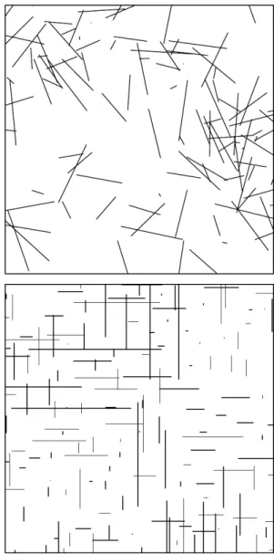
of the segmentXi+Ξi. Fig. 1 shows two realizations

of different models forΦ, observed through a square

window inR2.

Fig. 1.Two illustrations of realizations of planar line

segment processes.

If Φ is a stationary line segment process with

intensityλ, then there exists a probability distribution

Q(so calledtypical segment distribution) onS0 such

that

E

_∑

i≥1

f(Xi+Ξi) =λ Z

Rd

Z

S0

where f is an arbitrary nonnegative measurable

function onS. With only a slight abuse of notation,

we write Q also for the image of Q under the

isomorphism betweenS0and(0,∞)×L1. LetD(·) =

Q(· ×L1)andρ=Q((0,∞)× ·)be the distributions of

typical length and typical direction, respectively. The

distributionsD and ρ need not to be independent. In

what follows we call D the length distribution. It is

given by the cumulative distribution function

F(t) =Q({S:L(S)≤t}) =D([0,t]), t>0.

This paper deals with the estimation ofF. We consider

five existing nonparametric estimation methods.

If a line segment process Φ is defined by

an independently marked point process (Illian et

al., 2008, Section 5.1.3), i.e., {Ξi} is a sequence

of independent and identically distributed (= i.i.d.)

random segments, independent of{Xi}, then it is called

anindependent line segment process. A Poisson line segment processΦ={Xi+Ξi,i≥1}is an independent line segment process such that the germ process

{Xi,i≥1} is the Poisson point process (Illian et al.,

2008, Chapter 2) inRd. It follows from Theorem 3.5.7

in Schneider and Weil (2008) that the Poisson segment

process Φis the Poisson process in S (this space is

isomorphic toRd×S0).

A tractable class of models allowing dependencies among segments is obtained by geostatistical (or

external) marking, see Illianet al.(2008, Section 5.1.3)

for the definition in context of marked point processes.

Let{Ξ(x):x∈Rd}be a stationary random field with

values inS0, independent of{Xi}. We say that{Xi+

Ξ(Xi),i≥1}is ageostatistically marked line segment

process. The typical segment distributionQcoincides

with the distribution ofΞ(o).

MATERIAL AND METHODS

Usually we observe a single realization of the line

segment process Φ through a compact and convex

windowW ⊆Rd. Thus, the estimation is hampered by

edge effects which introduce spatial sampling bias. For example, if we consider all segments which intersect

W (with their true lengths), the final estimator of

the length distribution will be biased because longer segments have a greater chance to be included in the sample. On the other hand, if we consider just those segments which are completely inside the window,

segments longer than the diameter of W cannot be

sampled.

We can divide the line segments hitting W into

four groups: Y0 ={i:Xi+Ξi⊆W}, Y1 ={i:Xi ∈

W,e(Xi+Ξi)6∈W},Y2={i:Xi6∈W,e(Xi+Ξi)∈W},

Y3={i:Xi6∈W,e(Xi+Ξi)6∈W,(Xi+Ξi)∩W 6= /0}.

OnlyY0provides complete information about segment

lengths, in other cases the segments are not totally

observed. Directionsθ(Ξi)are observable for all line

segments hittingW. Segments corresponding toY0are

uncensored, segments from Y1 andY2 may be called

single end censored and segments fromY3 are called

double censored, see also Wijers (1997), p. 6.

Horvitz-Thompson type estimator

The sampling bias which is the result of the edge effects can be corrected by changing the sampling rule or by an appropriate weighting of the observations.

This leads us to theHorvitz-Thompson type estimator,

b FHT(t) =

1

b

λHT

∑

1

τ(Ξi)

1{L(Ξi)≤t},

where

bλ_HT=

∑

i:Xi+Ξi∈sample

1

τ(Ξi)

,

and τ is a suitable weighting function, i.e., τ(Ξi) =

R

1{x+Ξi ∈ sample}dx, see Baddeley (1999). As

a consequence of Eq. 1, b_λHTFbHT(t) is an unbiased

estimator of λF(t). Thus, FbHT(t) is a ratio of two

random variables so that the ratio of their expectations

isF(t). It means thatFbHT(t)is so-called ratio-unbiased

estimator of F(t). We will consider following three

basic sampling rules:

1) minus sampling – the sample consists of fully

observable segments (Xi+Ξi is sampled if and

only ifXi+Ξi⊆W),

2) unbiased sampling – the sample consists of segments with reference point inside the window

(Xi+Ξiis sampled if and only ifXi∈W),

3) plus sampling– the sample consists of all segments

hitting the window (Xi+Ξi is sampled if and only

if(Xi+Ξi)∩W 6=/0).

It means that minus sampling uses Y0, unbiased

sampling Y0∪Y1, and plus sampling Y0∪Y1∪Y2∪

Y3. The weights τ(Ξi) become |W Ξi| for minus

sampling, |W| for unbiased sampling, and |W⊕Ξi|

for plus sampling. Here, |B| is the d-dimensional

Lebesgue measure of the set B, B S0 = {x :x+

S0 ⊆ B} is the erosion of B by the line segment

S0 and B⊕S0 = {x : (x+S0)∩B 6= /0} is the

dilation of Bby the line segment S0. When applying

unbiased sampling or plus sampling rule, we need also some information outside the sampling window

W in order to determine Fb_HT. For independent line

segment processes, asymptotic properties of FbHT (as

the window W increases) follow from the results of

Reduced-sample estimator

For S ∈ S0 and t > 0, let ˜S(t) = _L(t_S)S be the

line segment in the same direction asSwith lengtht.

When estimatingF(t), a simple approach is to reduce

the sample and consider only those pairs (Xi,θ(Ξi))

for which the line segment Xi+Ξ˜

(t)

i with reference

point Xi, direction θ(Ξi) and length t would lie

completely inside the windowW. Then the

reduced-sample estimatorofF(t)can be defined by

b

F_rs(t) =∑i:Xi∈W1{L(Ξi)≤t,Xi+Ξ˜ (t)

i ⊆W}

∑i:Xi∈W1{Xi+Ξ˜ (t)

i ⊆W}

, t>0.

(2) This estimator takes into account only segments from

Y0 and Y1. Moreover, only the length of the visible

part is required for segments fromY1.

Since from Eq. 1,

E

_∑

i:X_i∈W

1{L(Ξi)≤t,Xi+Ξ˜

(t)

i ⊆W}

=λ Z

S0

|W S˜(t)|1{L(S)≤t}Q(dS),

the reduced-sample estimator is ratio-unbiased

provided thatQ=D×ρ. For largert, it may discard

a lot of information given by data. Note that it is not necessarily nondecreasing. The estimators of this type are often used in spatial statistics in order to deal with edge effects caused by the bounded observation

window, see, e.g. Baddeley (1999). This approach is

sometimes also called the border method for edge

correction.

Kaplan-Meier estimator

Random censoring and survival theory provide

us another look at the edge effects. Let {Ti} be

i.i.d. positive random variables (survival data) with

distribution function H. Instead of them we observe

only censored dataT_i0=min(Ti,Ci) and indicators of

non-censoringDi=1{Ti<Ci}. If we assume that{Ci}

are i.i.d. random variables, independent of {Ti}, then

the product-limit estimator defined as

b

H(t) =1−

_∏

s≤t

1−∑i≥11{T

0

i =s,Di=1}

∑i≥11{Ti0≥s}

!

is the nonparametric maximum likelihood estimate

of H(t). It is known as the Kaplan-Meier estimator

(Kaplan and Meier, 1958). In our context,Ti=L(Ξi)is

the true segment length andCiis the distance from the

reference point Xi to the boundary ofW in direction

θ(Ξi) of the line segment Xi+Ξi. It means that the

line segment Xi+Ξi is not censored (i.e., Di =1) if

Xi+Ξi ⊆W (i∈Y0). To avoid the sampling bias, let

us consider only those segments with reference point

inside the window W (i.e., i ∈Y0∪Y1). Then the

Kaplan-Meier estimatorofF is given by

b

FKM(t) =1−

∏

1−∑i≥11{Xi∈W,L(Ξi) =s,Xi+Ξi⊆W}

∑i≥11{Xi∈W,L((Xi+Ξi)∩W)≥s}

! .

This estimator for general germ-grain processes was introduced in Pawlas (2006). A related estimator is used in Laslett (1982a) for line segment processes. Since the independence assumptions are no longer satisfied, the optimality (in the sense of nonparametric maximum likelihood) of the Kaplan-Meier estimator is destroyed in our setting. An analogous situation happens in Baddeley and Gill (1997) where the empty space function and the nearest neighbour distance distribution function of spatial point processes are estimated. Baddeley and Gill (1997) show that the Kaplan-Meier technique provides reasonable

estimators. Similarly,FbKM(t)should yield an estimator

ofF(t) that is more efficient than the reduced-sample

estimatorFb_rs(t).

Nonparametric maximum likelihood estimator

A natural question is how the NPMLE of F(t)

looks like. Laslett (1982b) noted that it is not the Kaplan-Meier estimator and proposed a method of estimating the length distribution for stationary

Poisson segment processes inR2. The NPMLE of the

length distribution in a stationary planar Poisson line segment process was found by Wijers (1997) as the solution of the self-consistency equations that can be solved numerically by the expectation-maximization (EM) algorithm. We shortly describe the procedure

for the caseW = [0,a]2, for details see Wijers (1997).

Define

V(t) =

Z t

0

a2+auh(ρ)

a2_+aµh(ρ)dF(u), t>0,

where µ =R₀∞tD(dt) is the mean length of a typical

segment and h(ρ) = R₋π/2

π/2(cosθ +|sinθ|)ρ(dθ).

Here, we identifyL1with(−π/2,π/2]. In an isotropic

case (ρ is the uniform distribution),h(ρ) =_π4. Letn=

∑i1{(Xi+Ξi)∩W6=/0}be the number of observations

(number of line segments hittingW). We introduce the

Fn(0)(t) = 1

n_i:i

∑

0

1{L(Ξi)≤t},

Fn(1,2)(t) = 1

n_i:i∈

∑

1∪Y2

1{L((Xi+Ξi)∩W)≤t},

Fn(3)(t) = 1

n_i:i

∑

3

1{L((Xi+Ξi)∩W)≤t},

corresponding to uncensored, single end censored and double censored observations, respectively. The

NPMLE ˆVn of reparametrizationV satisfies the

self-consistency equation

d ˆVn(t) =dF

(0)

n (t)

+

Z t

0

1 ˆ

gn(u)

dFn(1,2)(u)

1

a2_+ath(ρ)d ˆVn(t)

+

Z t

0 t−u

ˆ

dn(u,u)

dFn(3)(u)

1

a2_+ath(ρ)d ˆVn(t),

(3)

where

ˆ

gn(u) =

Z ∞

u

1

a2_+awh(ρ)d ˆVn(w),

ˆ

dn(u,u) =

Z ∞

u

w−u

a2_+awh(ρ)d ˆVn(w).

Ifρ is assumed to be known, then a solution of Eq. 3

can be found using the EM algorithm. We start with

an initial estimator ˆV_n0 which sets positive mass to all

observation points. The iterative scheme of the EM

algorithm is obtained by replacing ˆVnwith ˆVnk+1on the

left hand side of Eq. 3 and by replacing ˆVn with ˆVnk

on the right hand side of Eq. 3. Now suppose that the

distributionρ of segment directions is unknown. The

NPMLE ˆρnofρ for givenFcan be expressed as

ˆ

ρn(η) =

∑ni=1(a2+aµ(cosθ(Ξi) +|sinθ(Ξi)|))

−1_1{

θ(Ξi)≤η}

∑ni=1(a2+aµ(cosθ(Ξi) +|sinθ(Ξi)|))−1

.

(4)

This leads us to a natural iterative scheme. For given ˆρnk

we determine ˆF_nk+1using the step of the EM algorithm

described above and for given ˆF_nk+1 we determine

ˆ

ρnk+1 from Eq. 4. The EM algorithm for estimation

of the length distribution is also used in Svensson et

al.(2006). We stress that Eq. 3 and Eq. 4 are derived

specifically ford=2.

Stochastic restoration estimation

Besides nonparametric estimators, one can also consider a parametric approach, where the length distribution is known up to a vector of unknown

parameters. Parametric estimation procedures were

studied, for example, by Chadœuf et al. (2000) who

propose so called stochastic restoration estimation

(SRE) algorithm. As it is mentioned in Chadœuf et

al.(2000), this Monte Carlo algorithm can be applied

also in the nonparametric setting. In order to avoid the sampling bias, we again take into account only the line

segments with reference point withinW. Denote their

number bym=|Y0|+|Y1|and consider the empirical

distribution function of observable lengths given by

ˆ

F0(t) =F (0,1)

m (t) = 1

m_i:X

∑

i∈W

1{L((Xi+Ξi)∩W)≤t}.

At iteration ptwo main steps are performed. The first

step (R-step) is the restoration of lengths of censored

segments (i ∈ Y1). It is made by simulation from

the conditional distribution with current estimate ˆFp,

we obtain lengths ˜Li. In the second step (E-step) the

estimate ˆF is updated by taking ˆFp+1 as the empirical

distribution function of uncensored segment lengths

L(Ξi), i∈ Y0, and restored lengths ˜Li, i∈ Y1. The

result of this algorithm is a homogeneous Markov

chain{_Fˆ_{p}. In practice, we define the SRE estimator}

as ˆFpfor some prescribed large p.

Simulations

A simulation study is conducted to compare the behaviour of individual estimators. Simulations and

computations are performed using R (R Core Team,

2018) and its contributed packagespatstat (Baddeley

and Turner, 2005). We generate six types of stationary

line segment processes inRd(withd=2 ord=3). The

point process of reference points {Xi} has intensity

λ >0 and is chosen as one of the following three

processes:

1) Poisson point process,

2) Mat´ern cluster process with mean number of points

per clusterµ =5 and radius of clustersR=0.1,

3) Mat´ern hard-core process II with hard-core

distanceh=0.05(d−1).

These three processes provide models for random, clustered and regular patterns, respectively. For the definition of Mat´ern cluster process we refer to

Illian et al. (2008, Section 6.3.2) or Schneider and

Weil (2008, p. 93). The definition of Mat´ern

hard-core process II can be found in Illian et al. (2008,

Section 6.5.2) or (Schneider and Weil, 2008, p. 94). Once we have a pattern of reference points, the segments are attached according to either independent or geostatistical marking. The length and direction of typical segment are assumed to be independent,

i.e.,Q=D×ρ. First we consider the isotropic case –

unchanged and only change the directions to get an anisotropic segment process. In particular, the uniform

distribution on d perpendicular directions parallel to

the axes is used, i.e., each canonical direction with

probability 1/d. This procedure gives us realizations

of six segment processes, which are denoted by 1i, 1a, 2i, 2a, 3i, 3a, where the numbers stand for Poisson (1), clustered (2), and regular (3) pattern while the letters stand for isotropic case (i) and anisotropic case (a). Furthermore, in order to have dependent lengths we use geostatistical marking as follows: we consider

a Gaussian random field {Z(x)} with zero mean

and exponential covariance function cov(Z(x),Z(y)) =

e−4kx−yk_{. We set L(}

Ξi) =0.25Φ(Z(Xi)), where Φ is

the cumulative distribution function of the standard

normal distribution. It means that to the point Xi we

assign a segment of lengthL(Ξi)and direction that is

independent of{Z(x)}and{Xi},i.e., the geostatistical

marking is only applied to the length while the independent marking is applied to the direction. The

length distribution is then uniform on(0,0.25).

The procedure is repeated 10 000 times for each simulation experiment. We study the influence of

intensityλ (values 25, 50, 75, 100 and 125 are used),

length distribution (either uniform on (0,0.25) or

exponential with mean 0.125) and dimension (d =2

ord=3).

We observe a realization of each process in the

unit square or unit cube windowW= [0,1]d_{. However,}

also the information about all segments hittingW is

recorded so that we can evaluate estimators based on plus sampling as well. Fig. 1 shows two examples of segment processes, a realization of the process 2i with geostatistically marked uniform lengths (left) and a realization of the process 3a with independently marked exponential lengths (right).

For every simulated segment pattern we determine all mentioned estimators:

(a) Horvitz-Thompson type estimator Fb_HT using

minus sampling,

(b) Horvitz-Thompson type estimator FbHT using

unbiased sampling,

(c) Horvitz-Thompson type estimator FbHT using plus

sampling,

(d) reduced-sample estimatorFbrs,

(e) Kaplan-Meier estimatorFbKM,

(f) nonparametric maximum likelihood estimator

assuming that the directions are uniformly

distributed (only ford=2),

(g) nonparametric maximum likelihood estimator for

unknown distribution of directions (only for d =

2),

(h) estimator obtained after p = 100 000 steps of

stochastic restoration estimation algorithm.

The estimators (b), (d), (e) and (h) depend on the choice of a reference point. Two natural choices are

lexicographic minimum point c(S) and lexicographic

maximum pointe(S). Thus, for each type of estimator

we can obtain the estimators ˆFc and ˆFe corresponding

to these choices as a reference point. We do not consider both estimators separately but we improve

them by taking the average 1₂(Fˆc+Fˆe). Since the

estimators (b) and (c) require information from outside

W, we include in the comparison with other estimators

only the minus sampling estimator (a). The estimators (f) and (g) were almost identical in all our experiments. So in what follows we only deal with (g). We run

106 iterations of the EM algorithm to evaluate this

estimator.

To measure the quality of the estimatorFb we use

two criterion functions that are used for goodness of fit tests (Stephens, 1992), the Kolmogorov–Smirnov statistic

dKS(Fb,F) = sup

t∈R+

|Fb(t)−F(t)|,

and the Cram´er–von Mises statistic

dCvM(Fb,F) =

Z ∞

0

(Fb(t)−F(t))2dF(t).

These deviation measures are computed for each simulated realization of line segment process for all estimators. In the forthcoming figures we present their sample means obtained from 10 000 repetitions for each process and each experiment.

RESULTS

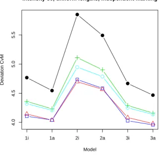
First we consider the case of independent line

segment process inR2. The best performance in most

scenarios was found for NPMLE. Only for the smallest

intensity (λ =25) and uniform length distribution it

was outperformed by the reduced-sample estimator.

For λ = 50 and uniform lengths, Fbrs has slightly

smaller values of meandCvM for some of the models.

The results of the comparison are shown in Fig. 2

(left for λ =50 and uniform length distribution and

right forλ =100 and exponential length distribution).

●

●

●

●

●

●

4.0

4.5

5.0

5.5

Intensity 50, uniform lengths, independent marking

Model

De

viation CvM

1i 1a 2i 2a 3i 3a

●

●

●

●

●

●

● _●

●

●

●

●

4

5

6

7

Intensity 100, exponential lengths, independent marking

Model

De

viation CvM

1i 1a 2i 2a 3i 3a

● _●

● _●

●

●

Fig. 2. The values of 1000·dCvM for six considered

models in case of independent marking, d = 2, uniformly distributed lengths and λ = 50 (top)

and exponentially distributed lengths and λ =

100 (bottom). Horvitz-Thompson (black, bullets), reduced-sample (red, triangles), Kaplan-Meier (green, crosses), NPMLE (blue, squares), and SRE (cyan, circles) estimators are compared.

patterns lead to lower values ofdKS and dCvM. Since

the NPMLE was derived under the assumption of Poisson segment process, it is not surprising that it has the smallest deviation from the true distribution function in that case. Under independent marking, we observed that the influence of underlying configuration of reference points is quite negligible. The NPMLE works very well also for clustered and regular patterns.

Comparing the remaining estimators, the reduced-sample estimator performed well for uniform length and smaller intensities while in other cases (uniform length and larger intensity, exponential length and arbitrary intensity) SRE and Kaplan-Meier estimator were better. Both these estimators gave very similar values, in particular for exponential lengths. The Horvitz-Thompson type estimator has the poorest behaviour among all studied estimators.

Similar conclusions could be made also for geostatistically marked line segment process. In this case the segments are dependent. However, the NPMLE still resulted in the lowest mean deviation measures. SRE and Kaplan-Meier estimator behave very similarly. The reduced-sample estimator was to some degree worse than in independent case. In some situations (especially with larger intensity) it was even beaten by the Horvitz-Thompson type estimator. The comparison for two different intensities is depicted in Fig. 3.

Finally, we have investigated the estimation for

independent line segment processes in R3. Since

the calculation of NPMLE is designed only for the planar case, it was not taken into account. The reduced-sample estimator shows the best behaviour for smaller intensities. For larger intensities reduced-sample estimator, Kaplan-Meier estimator, and SRE provide comparable results. The Horvitz-Thompson type estimator has again the largest mean deviation from true distribution function. Fig. 4 shows the comparison of results for two different intensities and uniformly distributed lengths.

●

●

●

●

●

●

0.23

0.24

0.25

0.26

0.27

Intensity 50, uniform lengths, geostatistical marking

Model

De

viation KS

1i 1a 2i 2a 3i 3a

●

●

●

●

●

●

●

●

●

●

●

●

21

22

23

24

25

26

Intensity 100, uniform lengths, geostatistical marking

Model

De

viation CvM

1i 1a 2i 2a 3i 3a

●

●

●

●

●

●

Fig. 3. The comparison of results for models

with geostatistical marking and uniformly distributed lengths. The values of dKS (top) and 1000·dCvM

(bottom) are shown for six considered models with λ = 50 (left) and λ = 100 (right). Horvitz-Thompson (black, bullets), reduced-sample (red, triangles), Kaplan-Meier (green, crosses), NPMLE (blue, squares) and SRE (cyan, circles) estimators are considered.

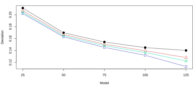
With increasing intensity we have more data and the estimators are more accurate. It is demonstrated in Fig. 6 where independent marking and exponentially distributed lengths are considered. The underlying point process is Mat´ern hard-core process II.

●

●

●

●

●

●

4.0

4.5

5.0

5.5

Intensity 50, 3D, uniform lengths, independent marking

Model

De

viation CvM

1i 1a 2i 2a 3i 3a

●

●

●

●

●

●

●

●

●

●

●

●

1.9

2.0

2.1

2.2

2.3

2.4

Intensity 100, 3D, uniform lengths, independent marking

Model

De

viation CvM

1i 1a 2i 2a 3i 3a

●

●

●

●

●

●

Fig. 4. The values of 1000·dCvM for six considered

models in case of independent marking, d = 3, uniformly distributed lengths and λ =50 (top) and λ =100(bottom). Horvitz-Thompson (black, bullets),

reduced-sample (red, triangles), Kaplan-Meier (green, crosses), and SRE (cyan, circles) estimators are compared.

DISCUSSION

We have reviewed several nonparametric

●

●

●

●

●

●

2.2

2.4

2.6

2.8

3.0

3.2

3.4

Horvitz−Thompson, intensity 75

Model

De

viation CvM

1i 1a 2i 2a 3i 3a

●

●

●

●

●

●

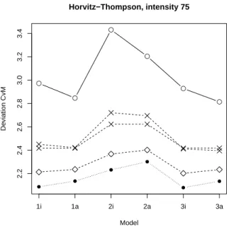
Fig. 5. The values of 1000·dCvM for six considered

models in case of independent marking, d = 2, uniformly distributed lengths and λ =75. Different

Horvitz-Thompson estimators are compared: minus sampling (full line, circles), unbiased sampling (dashed line, crosses for individual estimators and rhombi for average), and plus sampling (dotted line, bullets).

In the planar case, the nonparametric maximum likelihood estimator (NPMLE) is based on the assumption of Poisson process. Our simulation study revealed that this estimator is quite robust and preserves its superior behaviour also if the underlying point process is not Poisson and if the independence of segments is not satisfied. This estimator is computed using the EM algorithm that requires many iterations. However, its calculation is still quite fast (few seconds). Stochastic restoration estimation (SRE) requires an iterative numerical procedure as well. The computation time depends on the number of steps. In our experiments, the rate of convergence was quite

good. The results for p = 1 000 steps were almost

the same as for p=100 000 steps. The computation

time forp=1 000 was comparable with NPMLE (few

seconds). For larger number of steps the calculation of SRE becomes more time demanding (few minutes). Our aim was to find out whether simpler estimators can compete with NPMLE and SRE. These simpler estimators are very easy to implement and they are computed almost immediately. The Kaplan-Meier estimator gave results which are comparable with SRE in most scenarios. The reduced-sample estimator also provides a simple and reasonable alternative. It worked particularly well for lower values of intensity.

This estimator is less precise for larger t where

more information from data is discarded. Therefore, it behaves worse for exponential length in comparison with uniform length. Furthermore, the reduced-sample estimator, Eq. 2, is not necessarily monotonic. In that case, we suggest to use a natural modification

b

Frs,m=sup

s≤t

b

Frs(s), t>0.

Horvitz-Thompson type estimator was the least efficient estimator in our simulation study. It was expected because it uses only uncensored segments, single end censored segments are ignored.

In conclusion, we can recommend both

Kaplan-Meier and reduced-sample estimators when a

computationally simple method is required. They are also convenient in higher dimensions since the equations for the NPMLE are derived for the planar case.

ACKNOWLEDGEMENTS

We would like to thank the anonymous reviewers for their constructive suggestions and comments. The work is supported by the Grant Agency of the Czech Republic, project 16-03708S.

REFERENCES

Baddeley AJ (1999). Spatial sampling and censoring. In: Barndorff-Nielsen OE, Kendall WS, van Lieshout MNM, eds. Stochastic Geometry: Likelihood and Computation. London: Chapman and Hall, 37–78. Baddeley AJ, Gill RD (1997). Kaplan-Meier estimators of

distance distributions for spatial point processes. Ann Statist 25:263–92.

Baddeley AJ, Turner R (2005). Spatstat: anRpackage for analyzing spatial point patterns. J Stat Softw 12:1–42. Chadœuf J, Senoussi R, Yao JF (2000). Parametric

estimation of a Boolean segment process with stochastic restoration estimation. J Comput Graph Statist 9:390– 402.

Heinrich L, Pawlas Z (2008). Weak and strong convergence of empirical distribution functions from germ-grain processes. Statistics 42:49–65.

Illian J, Penttinen A, Stoyan H, Stoyan D (2008). Statistical Analysis and Modelling of Spatial Point Patterns. Chichester: John Wiley & Sons.

Kaplan EL, Meier P (1958). Nonparametric estimation from incomplete observations. J Amer Statist Assoc 53:457– 81.

●

●

●

●

●

0.12

0.14

0.16

0.18

0.20

Regular pattern, exponential lengths, independent marking

Model

De

viation

25 50 75 100 125

●

●

●

●

●

Fig. 6.The values of dKSfor different choices ofλin the case of independent line segment process in the plane with

regular pattern of reference points. Typical segment distribution is composed from two independent components: exponential length and isotropic direction. Horvitz-Thompson (black, bullets), reduced-sample (red, triangles), Kaplan-Meier (green, crosses), NPMLE (blue, squares), and SRE (cyan, circles) estimators are compared.

Laslett GM (1982a). Censoring and edge effects in areal and line transect sampling of rock joint traces. Math Geol 14:125–40.

Laslett GM (1982b). The survival curve under monotone density constraints with applications to two-dimensional line segment processes. Biometrika 69:153–60.

Pawlas Z (2006). Estimation of the distribution function in germ-grain models. In: Huˇskov´a M, Janˇzura M, eds. Proceedings Prague Stochastics 2006. Prague: Matfyzpress, 579–89.

Pawlas Z, Honzl O (2010). Comparison of length-intensity estimators for segment processes. Statist Probab Lett 80:825–33.

R Core Team (2018). R: A language and environment for statistical computing. R Foundation for Statistical Computing, Vienna, Austria. URL

https://www.R-project.org/.

Schneider R, Weil W (2008). Stochastic and Integral Geometry. Berlin: Springer-Verlag.

Stephens MA (1992). Introduction to Kolmogorov (1933) On the empirical determination of a distribution. In: Kotz S, Johnson NL, eds. Breakthroughs in Statistics: Methodology and Distribution. New York: Springer-Verlag, 93–105.

Svensson I, Sj¨ostedt-de Luna S, Bondesson L (2006). Estimation of wood fibre length distributions from censored data through an EM algorithm. Scand J Statist 33:503–22.

van Zwet EW (2004). Laslett’s line segment problem. Bernoulli 10:377–96.