DIRECT ONE-STEP METHOD FOR SOLVING THIRD-ORDER BOUNDARY VALUE PROBLEMS

(1)

ISSN: 1311-1728 (printed version); ISSN: 1314-8060 (on-line version) doi:_{http://dx.doi.org/10.12732/ijam.v32i2.1}

Athraa Abdulsalam1,3§_{, Norazak Senu}1,2_{, Zanariah Abdul Majid}1,2 1_{Department of Mathematics}

Universiti Putra Malaysia

43400 UPM Serdang, Selangor, MALAYSIA

2_{Institute for Mathematical Research}

Universiti Putra Malaysia

43400 UPM Serdang, Selangor, MALAYSIA

3_{Department of Mathematics}

University of Baghdad Al-Jadrriya, Baghdad, IRAQ

Abstract: A direct explicit Runge-Kutta type (RKT) method via shoot-ing technique to approximate analytical solutions to the third-order two-point boundary value problems (BVPs) with boundary condition type I and II are proposed. In this paper first, a three-stage fourth-order direct explicit Runge-Kutta type method denoted as RKT3s4 is constructed. A new algorithm of shooting technique for solving two-point BVPs for third-order ordinary differ-ential equations (ODEs) is presented.

AMS Subject Classification: 65L05, 65L06, 65L20

Key Words: direct Runge-Kutta method, two-point boundary value problem, shooting technique, third-order ordinary differential equation

Received: August 16, 2018 c 2019 Academic Publications

(2)

1. Introduction

Numerous problems in mathematics can be formulated in the form of differential equations, an initial value problem (IVP) is an ordinary differential equation (ODE) whose boundary conditions are specified at a single point, which can be found in mathematical modeling of real-life problems [1]-[3]. There is also another class of the ODE which is the boundary value problem (BVP), a BVP differs from an IVP in that the boundary conditions are specified at more than one point and in that solutions of the differential equation over an interval, satisfying the boundary conditions at the endpoints, are required ([4], p.1). BVP arises in several branches of engineering and applied sciences including fluid dynamics and chemical reactions, elastic beams, etc. (see [5], p.7 - p.27). In this work, we concentrate on finding an approximate solution to two-point BVPs with boundary conditions type I and II of the form

u′′′ =f(t, u), a < t < b, (1)

with boundary conditions: (a) Type I

u(a) =α, u′(a) =β, u(b) =γ. (2)

(b) Type II

u(a) =α, u′(a) =β, u′(b) =λ. (3)

(3)

multi-step, such methods are Predictor-Corrector methods, Adams-Moulton method, Adams -Bashforth method, and Trapezium rule method. Similarly, for the numerical procedures for the solution of the BVP, there exist several techniques, such as Finite-Difference method ([9], [10]), Shooting method ([5], [11]), the quasilinearization method ([12], [13]), the monotone iterative method ([14], [15]), and the variational iteration method ([16], [17]). Burden and Faires [1] have used RK method (after transferring it into the system of first-order) via shooting technique to solve second-order two-point linear BVP with Dirichlet boundary condition. However, many researchers ([18], [19]) have shown that using direct RK approach to solve higher-order ODE without reducing it first to a system of first-order is superior and more efficient than the conventional RK. Where there is no need to increase the number of equations and calculating more function evaluations which lead to a time-consuming process and more human effort as in classical RK.

Therefore, the purpose of this study is to construct a direct and effective method of Runge-Kutta type with less computation time and function evalua-tions to solve two-point BVPs of third-order with boundary condievalua-tions type I and II, algorithm of shooting technique was offered to develop the approximate analytical solutions.

The organizing of this paper is as follows: In Section 2, the construction of the explicit RKT3s4 method is presented. The explanation of the new shooting technique algorithm is given in Section 3. In Section 4, four problems numeri-cally examined the efficiency of the RKT3s4 method as compared to the existing method and the last section, deals with the conclusions.

2. Construction of the Explicit RKT3s4 Method

In this section, an explicit three-stage RKT method of order-four will be derived. The general µ-stage RKT method for the differential equation

u′′′ =f(t, u(t)) (4)

given by

un+1 = un+hu′n+

h2

2 u ′′

n+h3 µ X

i=1

biκi, (5)

u′_n+1 = u′_n+hu′′_n+h2

µ X

i=1

(4)

c1 0

c2 a21

c3 a31 a32

..

. ... ...

cµ aµ,1 aµ,2 . . . aµ,µ−1

b1 b2 . . . bµ−1 bµ

ˆ_b₁ ˆ_b₂ _{. . .} ˆ_b_µ₋₁ ˆ_b_µ ˆ

ˆ_b₁ ˆˆ_b₂ _{. . .} ˆˆ_b_µ₋₁ ˆˆ_b_µ

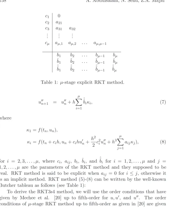
Table 1: µ-stage explicit RKT method.

u′′_n+1 = u′′_n+h

µ X

i=1

ˆ ˆ_b

iκi, (7)

where

κ1 =f(tn, un),

κi =f(tn+cih, un+cihu′n+

h2

2 c

2

iu′′n+h3 µ X

j=1

aijκj), (8)

for i = 2,3, . . . , µ, where ci, aij, bi, ˆbi, and ˆˆbi for i = 1,2, . . . , µ and j =

1,2, . . . , µ are the parameters of the RKT method and they supposed to be real. RKT method is said to be explicit when aij = 0 for i ≤ j, otherwise it

is an implicit method. RKT method (5)-(8) can be written by the well-known Butcher tableau as follows (see Table 1):

To derive the RKT3s4 method, we will use the order conditions that have given by Mechee et al. [20] up to fifth-order for u, u′_{, and} _u′′_{. The order} conditions of µ-stage RKT method up to fifth-order as given in [20] are given as follows.

The order conditions for u: Order 3:

X

bi=

1

6, (9)

Order 4:

X

bici=

1

(5)

Order 5:

X

bic2i =

1

60. (11)

The order conditions for u′_: Order 2:

X

ˆ_b_i₌ 1

2, (12)

Order 3:

X

ˆ_b_i_c_i₌ 1

6, (13)

Order 4:

X

ˆ_b_i_c2 i =

1

12, (14)

Order 5:

X

ˆ bic3i =

1 20,

X

ˆ biaij =

1

120. (15)

The order conditions for u′′_: Order 1:

Xˆ

ˆ_b_i_{= 1,} ₍₁₆₎

Order 2:

Xˆ

ˆ_b_i_c_i₌ 1

2, (17)

Order 3:

Xˆ

ˆ_b_i_c2 i =

1

3, (18)

Order 4:

Xˆ

ˆ_b_i_c3 i =

1 4,

Xˆ

ˆ biaij =

1

24, (19)

Order 5:

Xˆ

ˆ_b_i_c4 i =

1 5,

Xˆ

ˆ_b_i_a_ij_c_j ₌ 1 120,

Xˆ

ˆ_b_i_a_ij_c_i₌ 1

30. (20)

Now, assume that c3 = 1, as a result, we will have a system of nonlinear

equations, consisting of ten nonlinear equations with fourteen unknown vari-ables that have not yet been resolved, as follows:

b1+b2+b3 =

1

6, (21)

b2c2+b3c3 =

1

24, (22)

ˆ_b

1+ ˆb2+ ˆb3 =

1

(6)

ˆ_b₂_c₂_{+ ˆ}_b₃_c₃ ₌ 1

6, (24)

ˆ_b

2c22+ ˆb3c32 =

1

12, (25)

ˆ

ˆ_b₁₊ˆˆ_b₂₊ˆˆ_b₃ _{= 1,} ₍₂₆₎ ˆ

ˆ_b₂_c₂₊ˆˆ_b₃_c₃ ₌ 1

2, (27)

ˆ

ˆ_b₂_c₂2₊ˆ_ˆ_b 3c32 =

1

3, (28)

ˆ

ˆ_b₂_c₂3₊ˆ_ˆ_b 3c33 =

1

4, (29)

ˆ

ˆ_b₂_a_2,1₊ˆˆ_b₃_a_3,1₊ˆˆ_b₃_a_3,2 ₌ 1

24. (30)

Accordingly, the system has a solution based on three free parameters b2,

a2,1, and a3,1 as follows:

ˆ ˆ_b₁₌ 1

6, (31)

ˆ ˆ_b₂₌ 2

3, (32)

ˆ ˆ_b

3=

1

6, (33)

a3,2=−4a2,1−a3,1+

1

4, (34)

b1=

1 8 −

1

2b2, (35)

b3 =−

1 2b2+

1

24, (36)

c2 =

1

2, (37)

c3 = 1, (38)

ˆ_b

1 =

1

6, (39)

ˆ_b₂ ₌ 1

3, (40)

ˆ_b₃ _{= 0.} ₍₄₁₎

(7)

0

1 2 401

1 ₂₅1 ₁₀₀11 0

3

40 101 −1201

1

6 13 0

1

6 23 16

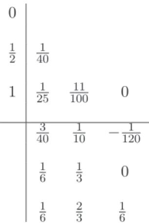
Table 2: Butcher tableau for RKT3s4 method.

follows:

kT_g(5)k2= v u u u t

n′′

p+1

X

i=1

(T_i′′(5))2₊ n′

p+1

X

i=1

(T_i′(5))2₊ np+1

X

i=1

(T_i(5))2_, ₍₄₂₎

where T′′(5)_, _T′(5)_{, and} _T(5) _{are the local truncation error terms of the RKT}

methods for u′′_,_u′_{, and} _u _{respectively and} _T(5)

g is the global truncation error.

Based on the free parameters b2, a2,1, and a3,1 we get the global truncation

error term of fifth-order condition for u,u′_, _u′′ _{as follows:}

kT_g(5) k2 =

1

240(19200a

2

2,1 + 3200a2,1a3,1+ 400a23,1+ 3600b22

−1120a2,1−120a3,1−720b2+ 61)1/2. (43)

Then, minimizing equation (43) with respect to the free parametersb2,a2,1,

anda3,1by using Maple software (Minimize command in Optimization package)

to obtain b2 = ₁₀1, a2,1 = ₁₀₀₀25 , a3,1 = ₁₀₀4 , and k Tg(5) k2= 0.01181453907.

Lastly, all the coefficients of the RKT3s4 method are written in Butcher tableau (see Table 2):

3. Shooting Method for Linear BVP

(8)

the other end converges to its correct value. When we use the shooting method, we transform (1) into IVP of the form

u′′′ =f(t, u), a < t < b,

u(a) =α, u′(a) =β, u′′(a) =λ1,

where λ1 is any number. Then the resulting IVP will be solved using RKT

method.

Reduction to Three IVPs:

The solution of a linear two-point BVP is associated with the formation of a linear combination of the solutions to three IVPs.

The form of the IVPs as follows.

Suppose that ψ(t) is the unique solution to the IVP

ψ′′′ =f1(t, ψ),

f1(t, ψ) =q(t)ψ(t) +g(t), with ψ(a) =α, ψ′(a) = 0, ψ′′(a) = 0. (44)

Suppose that ρ(t) is the unique solution to the IVP

ρ′′′ ₌_f

2(t, ρ),

f2(t, ρ) =q(t)ρ(t), with ρ(a) = 0, dρ′(a) = 1, ρ′′(a) = 0. (45)

Suppose that ϑ(t) is the unique solution to the IVP

ϑ′′′ ₌_f

3(t, ϑ),

f3(t, ϑ) =q(t)ϑ(t), with ϑ(a) = 0, ϑ′(a) = 0, ϑ′′(a) = 1. (46)

Then the linear combination

u(t) =ψ(t) +θ1ρ(t) +θ2ϑ(t), (47)

is a solution to the BVP (1).

For the boundary condition type I, the solution u(t) in equation (47) takes on the boundary values. Then the linear combination

u(a) =ψ(a) +θ1ρ(a) +θ2ϑ(a), (48)

u(a) =α. (49)

(9)

u′(a) =θ1. (51)

u(b) =ψ(b) +θ1ρ(b) +θ2ϑ(b). (52)

Imposing the boundary conditions u′_{(a) =} _β _and _{u(b) =} _γ _{in (51) and (52)} produces θ1 = β and θ2 = γ−ψ(b)_ϑ(b)−βρ(b). Therefore, if ϑ(b) 6= 0, the unique

solution of the two-point BVP (1) with boundary condition type I is given by:

u(t) =ψ(t) +βρ(t) +γ−ψ(b)−βρ(b)

ϑ(b) ϑ(t). (53)

For the boundary condition type II, the solution u(t) in equation (47) takes on the boundary values. Then the linear combination

u(a) =ψ(a) +θ1ρ(a) +θ2ϑ(a), (54)

u(a) =α, (55)

u′(a) =ψ′(a) +θ1ρ′(a) +θ2ϑ′(a), (56)

u′(a) =θ1. (57)

u′(b) =ψ′(b) +θ1ρ′(b) +θ2ϑ′(b). (58)

Imposing the boundary conditions u′_{(a) =} _β _and _u′_{(b) =} _λ _{in (57) and (58)} produces θ1 = β and θ2 = γ−ψ

′_(b)₋_βρ′_(b)

ϑ′_(b) . Therefore, if ϑ′(b) 6= 0, the unique solution of the two-point BVP (1) with boundary condition type II is given by:

u(t) =ψ(t) +βρ(t) + γ−ψ

′_(b)₋_βρ′_(b)

ϑ′_(b) ϑ(t). (59)

Algorithm 1: RKT Method via Linear Shooting Technique:

To approximate the solution of BVP (1) with boundary condition type I: INPUT:α,β,γ boundary conditions;a,bendpoints;N number of subintervals. OUTPUT: approximations ϕ1,i to u(ti) ; ϕ2,i to u′(ti) ; ϕ3,i to u′′(ti) for each

i= 0,1, ..., N.

Step 1: Seth= (b−a)/N;

ψ1,0 =α;

ψ2,0 = 0;

ψ3,0 = 0;

(10)

ρ2,0 = 1;

ρ3,0 = 0;

ϑ1,0= 0;

ϑ2,0= 0;

ϑ3,0= 1.

Step 2: For i= 0, . . . , N −1 do Step 3 and Step 4. (RKD method is used in Step 3 and Step 4.) Step 3: Sett=a+ih.

Step 4: Set

κ1 = f1(t, ψ1,i);

κi = f1(t+cih, ψ1,i+cihψ2,i+

h2

2 c

2

i ψ3,i+h3 i−1 X

j=1

aijκj);

ψ1,i+1 = ψ1,i+h ψ2,i+

h2

2 ψ3,i+h

3 µ X

i=1

biκi;

ψ2,i+1 = ψ2,i+h ψ3,i+h2 µ X

i=1

ˆ_b_i_κ_i_;

ψ3,i+1 = ψ3,i+h µ X

i=1

ˆ ˆ_b_i_κ_i_;

¯

κ1 = f2(t, ρ1,i);

¯

κi = f2(t+cih, ρ1,i+cihρ2,i+

h2 2 c

2

iρ3,i+h3 i−1 X

j=1

aijκ¯j);

ρ1,i+1 = ρ1,i+h ρ2,i+ h 2

2 ρ3,i+h

3 µ X

i=1

biκ¯i;

ρ2,i+1 = ρ2,i+h ρ3,i+h2 µ X

i=1

ˆ biκ¯i;

ρ3,i+1 = ρ3,i+h µ X

i=1

ˆ ˆ_b_i_κ_¯_i_;

¯ ¯

(11)

¯ ¯

κi = f3(t+cih, ϑ1,i+cih ϑ2,i+

h2

2 c

2

iϑ3,i+h3 i−1 X

j=1

aijκ¯¯j);

ϑ1,i+1 = ϑ1,i+h ϑ2,i+

h2

2 ϑ3,i+h

3 µ X

i=1

biκ¯¯i;

ϑ2,i+1 = ϑ2,i+h ϑ3,i+h2 µ X

i=1

ˆ_b_iκ¯¯i;

ϑ3,i+1 = ϑ3,i+h µ X

i=1

ˆ ˆ_b

iκ¯¯i;

Step 5: (For boundary condition type I)

setϕ1,0 =α ;

ϕ2,0 =β;

ϕ3,0= (γ−ψ1,N_ϑ1−_,Nϕ2,0ρ1,N) ;

OUTPUT (a, ϕ1,0, ϕ2,0, ϕ3,0).

Step 5: (For boundary condition type II)

setϕ1,0 =α ;

ϕ2,0 =β;

ϕ3,0= (γ−ψ2,N_ϑ2−_,Nϕ2,0ρ2,N) ;

OUTPUT (a, ϕ1,0, ϕ2,0, ϕ3,0).

Step 6: For i= 1, . . . , N set

Ω1 =ψ1,i+ϕ2,0ρ1,i+ϕ3,0ϑ1,i;

Ω2 =ψ2,i+ϕ2,0ρ2,i+ϕ3,0ϑ2,i;

Ω3 =ψ3,i+ϕ2,0ρ3,i+ϕ3,0ϑ3,i;

t=a+ih;

OUTPUT (t,Ω1,Ω2, ,Ω3).

(12)

4. Numerical Results

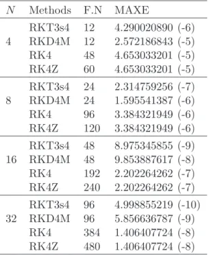
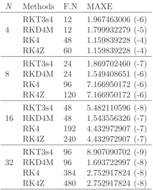
In this section, we selected four problems to test the performance of the RKT3s4 method in terms of accuracy and effectiveness. The first two problems are BVP problems, while the second problems are a class of BVP called self-adjoint singularly perturbed boundary value problems (SPBVPs).

For the numerical comparisons, we chose the following fourth-order RK types methods of comparisons for the first and second problems, whereas for SPBVPs we wanted to examine whether the new method could solve this type of problem or not, for this we compared with Quartic B-spline methods. Taking into consideration that the Quartic B-spline and Runge-Kutta type methods have different behavior.

All calculations were performed using the code written by us in C program.

• RKT3s4: The three-stage fourth-order explicit RKT method derived in this paper;

• RKD4M:The three-stage fourth-order RKT method of [23]; • RK4: The four-stage fourth-order RK method given in [22]; • RK4Z:The five-stage fourth-order RK method of [24]; • F.N:The number of function evaluations;

• MAXE: Max (|y(tn) −yn|) which is the maximum between absolute

errors of the exact solutions and the computed solutions;

Problem 1. (See Arshad et al. [25]) Consider the inhomogeneous linear two-point BVP

u′′′ ₌_tu_{+ (t}3₋_2t2₋_5t₋_3)et_, ₀_≤_t_≤_1,

u(0) = 0, u′(0) = 1, u(1) = 0.

The analytic solution is given by

u(t) =t(1−t)et.

Problem 2. (See Abd El-Salam et al. [26]) Consider the inhomogeneous linear two-point BVP

(13)

u(t) =(t−1) sint.

Problem 3. (See Saini et al. [27]) Consider the inhomogeneous two-point SPBVP

−ǫu′′′+u= 6ǫ(1−t)5t3−6ǫ2

6 (1−t)5−90 (1−t)4t

+ 180(1−t)3t2−60 (1−t)2t3

,

u(0) = 0, u′(0) = 0, u(1) = 0.

u(t) = 6t3ǫ(1−t)5.

Problem 4. (See Saini et al. [27]) Consider the inhomogeneous two-point SPBVP

−ǫu′′′+u= 81ǫ2cos 3t+ 3ǫsin 3t,

u(0) = 0, u′(0) = 9ǫ, u(1) = 3ǫsin(3).

u(t) = 3ǫsin 3t.

(14)

N Methods F.N MAXE

RKT3s4 12 4.290020890 (-6)

4 RKD4M 12 2.572186843 (-5)

RK4 48 4.653033201 (-5)

RK4Z 60 4.653033201 (-5)

RKT3s4 24 2.314759256 (-7)

8 RKD4M 24 1.595541387 (-6)

RK4 96 3.384321949 (-6)

RK4Z 120 3.384321949 (-6)

RKT3s4 48 8.975345855 (-9)

16 RKD4M 48 9.853887617 (-8)

RK4 192 2.202264262 (-7)

RK4Z 240 2.202264262 (-7)

RKT3s4 96 4.998855219 (-10)

32 RKD4M 96 5.856636787 (-9)

RK4 384 1.406407724 (-8)

RK4Z 480 1.406407724 (-8)

Table 3: Maximum errors and number of function evaluations of Problem 1.

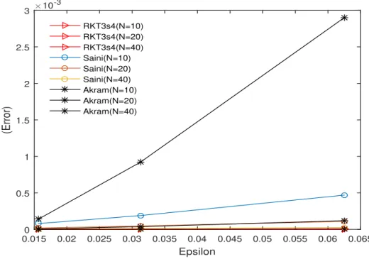
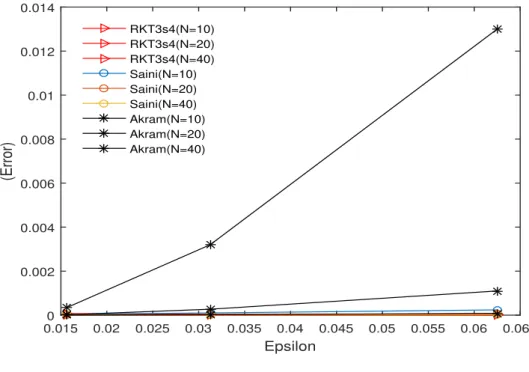
save a large amount of work, in terms of the number of function evaluations. As for solving third order SPBVP with respect to different values of ǫ, we observed that the results obtained in Tables 5, 8 showed the efficiency of the new method. Figures 3, 4 are also visualized comparing the given tables. Thus, the RKT3s4 method is very efficient and accurate to evaluate according to the given problems and boundary conditions.

5. Conclusion

(15)

N Methods F.N MAXE

RKT3s4 12 1.967463006 (-6)

4 RKD4M 12 1.799932279 (-5)

RK4 48 1.159839228 (-4)

RK4Z 60 1.159839228 (-4)

RKT3s4 24 1.869702460 (-7)

8 RKD4M 24 1.549408651 (-6)

RK4 96 7.166950172 (-6)

RK4Z 120 7.166950172 (-6)

RKT3s4 48 5.482110596 (-8)

16 RKD4M 48 1.543556326 (-7)

RK4 192 4.432972907 (-7)

RK4Z 240 4.432972907 (-7)

RKT3s4 96 8.907090702 (-9)

32 RKD4M 96 1.693722997 (-8)

RK4 384 2.752917824 (-8)

RK4Z 480 2.752917824 (-8)

Table 4: Maximum errors and number of function evaluations of Problem 2.

N ǫ=1/16 ǫ=1/32 ǫ =1/64

10 6.5×10−6 _2.8_×₁₀−6 _1.0_×₁₀−6

20 4.2×10−7 _1.7_×₁₀−7 _6.6_×₁₀−8

40 2.6×10−8 _1.1_×₁₀−8 _4.1_×₁₀−9

Table 5: Maximum error of RKT3s4 of Problem 3.

(16)

N ǫ=1/16 ǫ=1/32 ǫ =1/64

10 4.7×10−4 1.9×10−4 8.0×10−5 20 1.1×10−4 _4.7_×₁₀−5 _1.9_×₁₀−5

40 2.6×10−5 _1.2_×₁₀−5 _4.8_×₁₀−6

Table 6: Maximum error of Problem 3 in Saini [27].

N ǫ=1/16 ǫ=1/32 ǫ =1/64

10 2.9×10−3 _9.2_×₁₀−4 _1.4_×₁₀−4

20 1.2×10−4 _3.8_×₁₀−5 _6.8_×₁₀−6

40 6.4×10−6 _2.1_×₁₀−6 _4.6_×₁₀−7

Table 7: Maximum error of Problem 3 in Akram [28].

N ǫ=1/16 ǫ=1/32 ǫ =1/64

10 1.9×10−5 _3.7_×₁₀−5 _7.0_×₁₀−5

20 2.6×10−6 _5.0_×₁₀−6 _9.9_×₁₀−6

40 3.4×10−7 _6.6_×₁₀−7 _1.3_×₁₀−6

Table 8: Maximum error of RKT3s4 of Problem 4.

N ǫ=1/16 ǫ=1/32 ǫ =1/64

10 2.4×10−4 _1.0_×₁₀−4 _4.0_×₁₀−5

20 6.1×10−5 _2.6_×₁₀−5 _1.0_×₁₀−6

40 1.5×10−5 _6.4_×₁₀−6 _2.5_×₁₀−6

Table 9: Maximum error of Problem 4 in Saini [27].

Acknowledgements

(17)

Min-N ǫ=1/16 ǫ=1/32 ǫ =1/64

10 1.3×10−2 3.2×10−3 3.4×10−4 20 1.1×10−3 _2.7_×₁₀−4 _2.2_×₁₀−5

40 7.8×10−5 _1.8_×₁₀−5 _1.1_×₁₀−6

Table 10: Maximum error of Problem 4 in Akram [28].

log

10(Number of function evaluations)

1 1.2 1.4 1.6 1.8 2 2.2 2.4 2.6 2.8

log

1

0

(Max global error)

-10 -9 -8 -7 -6 -5 -4

RKT3s4 RKD4M RK4 RK4Z

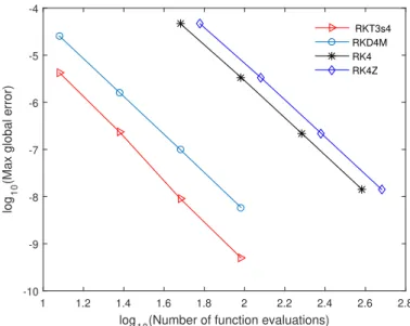
Figure 1: The efficiency curve for RKT3s4, RKD4M, RK4, and RK4Z for Problem 1 withN = 2i_{, i}_{= 2,} _3,_4,_5.

istry of Education.

References

[1] R.L. Burden, J.D. Faires, Numerical Analysis, Brooks/Cole, Cengage Learning, Boston (2011).

(18)

second-log

10(Number of function evaluations)

1 1.2 1.4 1.6 1.8 2 2.2 2.4 2.6 2.8

log

1

0

(Max global error)

-8.5 -8 -7.5 -7 -6.5 -6 -5.5 -5 -4.5 -4 -3.5

RKT3s4 RKD4M RK4 RK4Z

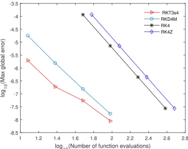
Figure 2: The efficiency curve for RKT3s4, RKD4M, RK4, and RK4Z for Problem 2 withN = 2i, i= 2, 3,4,5.

order ordinary differential equations, Discrete Dynamics in Nature and Society,2018 (2018), 10 pages.

[3] N. Ghawadri, N. Senu, F. Ismail and Z.B. Ibrahim, Exponentially fitted and trigonometrically fitted explicit modified Runge-Kutta type methods for solving y′′′ ₌ _f_{(x, y, y}′_), _{J. of Applied Mathematics}_, ₂₀₁₈ _{(2018), 19} pages.

[4] T.Y. Na, Computational Methods in Engineering Boundary Value Prob-lems,Academic Press, New York (1980).

[5] U.M. Ascher, R.M.M. Mattheij and R.D. Russell, Numerical Solution of Boundary Value Problems for Ordinary Differential Equations, SIAM, Philadelphia (1994).

[6] P. Henrici, Discrete Variable Methods in Ordinary Differential Equations, Wiley, New York (1962).

(19)

Epsilon

0.015 0.02 0.025 0.03 0.035 0.04 0.045 0.05 0.055 0.06 0.065

(Error)

×10-3

0 0.5 1 1.5 2 2.5 3

RKT3s4(N=10) RKT3s4(N=20) RKT3s4(N=40) Saini(N=10) Saini(N=20) Saini(N=40) Akram(N=10) Akram(N=20) Akram(N=40)

Figure 3: Comparison figure between RKT3s4, Saini, and Akram methods.

[8] A. Dhamacharoen and K. Chompuvised, An efficient method for solving multipoint equation boundary value problems,World Academy of Science, Engineering and Technology,75(2013), 61-65.

[9] I.A. Tirmizi and E.H. Twizell, Higher-order finite-difference methods for nonlinear second-order two-point boundary-value problems,Applied Math-ematics Letters,15, No 7 (2002), 897-902.

[10] A. Pierluigi and I. Sgura, High-order finite difference schemes for the solu-tion of second-order BVPs,J. of Computational and Applied Mathematics,

176, No 1 (2005), 59-76.

[11] S.N. Ha, A nonlinear shooting method for two-point boundary value prob-lems, Computers and Mathematics with Applications, 42, No 10 (2001), 1411-1420.

(20)

Epsilon

0.015 0.02 0.025 0.03 0.035 0.04 0.045 0.05 0.055 0.06 0.065

(Error)

0 0.002 0.004 0.006 0.008 0.01 0.012 0.014

RKT3s4(N=10) RKT3s4(N=20) RKT3s4(N=40) Saini(N=10) Saini(N=20) Saini(N=40) Akram(N=10) Akram(N=20) Akram(N=40)

Figure 4: Comparison figure between RKT3s4, Saini, and Akram methods.

method for mixed boundary value problems, Applied Mathematics and Computation,133, No 2 (2002), 423-429.

[13] R.A. Khan, The generalized quasilinearization technique for a second order differential equation with separated boundary conditions, Mathematical and Computer Modelling,43, No 7 (2006), 727-742.

(21)

[17] Z.M. Odibat and S. Momani, Variational iteration method for solving non-linear boundary value problems, Applied Mathematics and Computation,

183, No 2 (2006), 1351-1358.

[18] S.N. Jator, Numerical integrators for fourth order initial and boundary value problems,International J. of Pure and Applied Mathematics,47, No 4 (2008), 563-576.

[19] K. Hussain, F. Ismail and N. Senu, Solving directly special fourth-order ordinary differential equations using Runge-Kutta type method,J. of Com-putational and Applied Mathematics, 306(2016), 179-199.

[20] M. Mechee, N. Senu, F. Ismail and B. Nikouravan, A three-stage fifth-order Runge-Kutta method for directly solving special third-fifth-order differ-ential equation with application to thin film flow problem, Mathematical Problems in Engineering,2013 (2013), 7 pages.

[21] J.R. Dormand and P.J. Prince, A family of embedded Runge-Kutta for-mulae, J. of Computational and Applied Mathematics, 6, No 1 (1980), 19-26.

[22] J.C. Butcher, Numerical Methods for Ordinary Differential Equations, John Wiley and Sons Ltd., England (2008).

[23] M. Mechee, F. Ismail, Z.M. Hussain and Z. Siri, Direct numerical meth-ods for solving a class of third-order partial differential equations,Applied Mathematics and Computation,247 (2014), 663-674.

[24] E. Hairer, S.P. Nrsett and G. Wanner,Solving Ordinary Differential Equa-tions,Springer-Verlag, Berlin (1993).

[25] A. Khan and T. Aziz, The numerical solution of third-order boundary-value problems using quintic splines, Applied Mathematics and Computa-tion,137, No 2 (2003), 253-260.

[26] F.A.A. El-Salam, A.A. El-Sabbagh and Z.A. Zaki, The numerical solution of linear third order boundary value problems using nonpolynomial spline technique,J. of American Science,6, No 12 (2010), 303-309.

(22)