Abstract— Human mobility in urban area related to how people moved from a city to another city, whether by walking or using vehicles to support their mobility. By processing data of human mobility, we can determine prediction of the next pattern of human mobility. Some methods for human mobility prediction have been proposed. One of them is predication using Markov. In this research, we conducted implementation of Markov algorithm to predict location of human mobility based on input data form individual mobility dataset (GeoLife) from GPS. The data used in this study is data of one individual with code (001). There are 71 trajectories with a total of 108607 points obtained from 2008-10-23 to 2008-12-15. This research carried out through five stages of research. The conclusions drawn from this study are the values for parameters such as HMM n_components = 5, covariance_type = 'spherical', and decoder algorithm = 'viterbi' which produces a curation of 0.769 and RMSE 1.641 can be said to be hmm good enough in modeling data.
Index Terms— Markov predictor, human mobility, prediction, statistical models
I. INTRODUCTION
Human mobility in the urban area related to how people moved from a city to another city, whether by walking or using vehicles to support their mobility [1]. In recent years, human mobility is started to be a research topic. The data regarding mobility is collected for research, for example, data movement from GPS in smartphones. By using this data, we can track human mobility based on their current location and geolocation that saved in social media. This human mobility data can be used to handle the problem in an urban area and as reference for urban planning [2][3][4].
By processing data of human mobility, we can determine the prediction of the next pattern of human mobility. Some methods for human mobility prediction have been proposed. One of them is predication using Markov. Markov prediction order-k O(k) can be used to predict the next location that will be visited by people based on the history of a location.
A preliminary study on human mobility was conducted in 2016. This initial study was conducted to understand the concept of the human mobility system, by using input data in the form of spatial coordinates on Twitter social media networks. In this preliminary research also provided out investigations of patterns of human movement based on geo-location predictions collected from Twitter. The process of
research is data retrieval including the parsing of raw twitter data, pre-processing to detect the temporal-spatial data, clustering of pre-processed data, and trajectory determination based on the geo-tagged sequence of tweets [2][3][4].
In this research, we handled the implementation of Markov algorithm to predict the location of human mobility based on input data form individual mobility dataset (GeoLife) from GPS. The results can be used as analytical material to define the point of interest of a group of people at a specified period.
II. LITERATURE REVIEW A. Markov Predictor
The issue of prediction in research has got attention through the past years, utilizing techniques including pattern matching, learning automata, or Kalman filtering [5], [6]. However, three algorithms are simple but there are weaknesses to complete some problems. For example, learning automata cannot tackle slow convergence to the correct actions [7]. Kalman filtering cannot be tackle problem to request prediction, but only for location prediction. Moreover, this filtering performance primarily based on the stabilization time of the Kalman filter and knowledge (or estimation) of the system’s parameters [8]. Finally, pattern matching techniques have been used for location prediction [8].
Therefore, Markov predictors more appropriate for carrying out location prediction/request prediction because they are domain independent, and a simple mapping from the “entities” of the investigated domain to an alphabet is all that is required. Thus, they can support both location and request prediction.
Markovian prediction relies on the short memory principle, which says that the (empirical) probability distribution of the next symbol, given the preceding sequence, can be quite accurately approximated by observing no more than the last few symbols in that sequence. This principle fits reasonably and intuitively with how humans are acting when traveling or seeking information. A mobile user usually travels with a specific destination in mind, designing its travel via specific routes (e.g., roads). This “targeted” traveling is far from a random walk assumption, and studies confirm it with real mobility traces [9]. Similarly, almost all request traces exhibit strong spatial locality, which describes correlated sequences of requests.
Hidden Markov model is a statistical model used to describe the Markov process with unknown parameters. It is often used to look for some changing patterns in a period
Prediction Using Markov for Determining
Location of Human Mobility
Vina Ayumi, Ida Nurhaida
and analysis of a system. The state which we hope to predict is hidden in the appearance and is not what we observed, for example, by observing the appearance of algae to predict the change of weather. Here, there are two kinds of state, observed state (the state of algae), hidden state (the state of weather). The difficulty is to determine the implicit parameters of the process from the observable parameters, and then use these parameters to do further analysis [10]:
1. The hidden states , which meet the Markov property, where N indicates the number of hidden states.
2. The observed states , associated with hidden states in the model, which can be obtained by direct observation (the number of observed states is not necessarily equal to the number of hidden states), where M is denoted as the number of observable states.
3. The initial state probability matrix π describes hidden state probability matrix when in the initial timestamp
t=1, where ,
initial state probability matrix π=[ π1, π2, π3 ]. 4. The transition probability matrix A of hidden states,
represents the transition probability between hidden
states in HMM, with equation ,
indicates that in timestamp t+1, the probability of state , in the condition of state Si in timestamp t. 5. The Confusion Matrix B of observed states, describes the transition probability between the hidden states and observed states in HMM, where is equation of the probability of observed state Oi is in the condition of hidden state S j in timestamp t [10].
Figure 1 is a state transition diagram of HMM, where
are hidden states, are observed
states, where a represents the state transition probability of hidden states, and b represents the transition probability between the hidden states and the observed states [10].
Fig. 1 State transition diagram [10]
B. Related Work
This study will use Markov Predictor to predict human mobility location and examine how Markov Predictor performance in processing human mobility dataset.
The statistical model has been proposed for human mobility, for example, Giannotti et al. [11], Qu et al. [12] and Cui et al. [13]. In this research, we proposed a statistical model name Markov Predictor. The background to choose this method because Markov Predictor has been successfully implemented as a solution for various case studies has been carried out, including wireless networks [7], electric load forecasting [14], and cognitive radio [15].
In field of human mobility, hidden Markov model have been proposed to work out the problem of location recognition and prediction [16][17][18]. Mathew et al. presented a hybrid method for predicting human mobility on the basis of HMM. The study approached clusters location histories correspond to their characteristics, and then trains an HMM for each cluster. In their study, they conduct a series of experiments using dataset from the GeoLife project and showing that accuracy of prediction is 13.85% achieved when considering regions of about 1280 square meters [16]. Simmons et al. presented a novel approach to predicting driver intent that exploits the predictable nature of everyday driving [17]. They proposed HMM to build a mode of the routes and destinations used by the drivers using a low-cost GPS sensor and a map database. They showed that the model can be used to make accurate prediction of the driver route and destination. Asahara et al. proposed a method for predicting pedestrian movement using the basis of a mixed Markov-chain model (MMM). They compared the proposed MMM-based prediction method and hidden-Markov model (HMM). The proposed method (MMM) reach the highest prediction accuracy is 74.4% [18].
III. METHODOLOGY
The research entitled Markov-based Predictions to Know the Location of Human Mobility is carried out through five stages of research as shown in Figure 4.2. This research conducted between December 2018 until March 2019.
Fig. 2 Research Phase
Data
Collection
processing
Data
Pre-Modelling
Testing
A description of each stage of the research is explained as follows:
1. Data collection
The data collection phase is done by finding the appropriate dataset, namely the public dataset from GeoLife GPS Trajectories.
2. Pre-process
This stage is carried out by detecting stay points, extracting the region of interest.
3. Modeling
This stage is done by building a model using the Markov prediction algorithm.
4. Testing
This stage is done by testing the model by predicting the test data. The prediction is done by estimating which location someone will visit next in a city. 5. Evaluation
The evaluation phase is done by evaluating the results of the predictions produced in the previous stage. The metric evaluation error used is symmetric Mean Absolute Percentage Error (sMAPE). The sMape is an error metric that is commonly used to evaluate errors in the prediction of a prediction of ground truth data.
A. Dataset
GeoLife dataset is a GPS trajectory dataset that collected by Microsoft Research Asia project. The dataset consist of 178 users in a period of over five years from (from April 2007 to August 2012) [19][20][21]. In this dataset, a GPS trajectory is represented by a sequence of time-stamped points, each of which contains the information of latitude, longitude and altitude. The dataset contains 17,621 trajectories with a total distance of about 1,292,951 kilometers and a total duration of 50,176 hours. Recorded by different GPS loggers and GPS-phones, the trajectories have a variety of sampling rates. As much as 91.5% of the trajectories being logged in a dense
representation, e.g. every 1-5 seconds or every 5-10 meters per point. GeoLife dataset recorded a wide range of outdoor movements by users, included not only life routines such as go to work and go home but also some entertainments and sports activities, like shopping, dining, sightseeing, cycling, and hiking [19][20][21].
B. Preprocessing
In this stage of preprocessing, after we cleaned the data, then we conducted the stay points detection and region of interest extraction.
1. Detecting Stays Points
In this phase we detect several stay point from a GPS trajectory of a user in period of over five years. A stay points is a geographic place where a user stays for a period of time. To detect stay points, two parameters are required, they are time (ϴt) and distance (ϴd) threshold. The time threshold and distance threshold that we used is 30 minutes and 200 meters. If time interval and distance of two points matches with the threshold condition, then the points will be merged into one stay point by replacing them with the center of point.
2. Extracting Region of Interest
In this stage we used DBScan algorithm to cluster region of interest from stay points. We calculate the clusters of stay points that are close to each other using this algorithm. The parameters to this algorithm are epsilon (eps) and minimum samples (min_samples). The epsilon parameter is the maximum distance between points so that can be considered as a cluster. In this study we used 1.5 km as the maximum distance of points can be considered as a cluster, and the min_samples is 1.
IV. RESULT
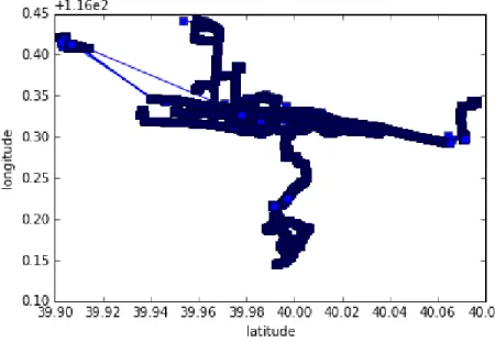
Fig. 3 Trajectory user 001
1. Detecting Stays Points
From all trajectory data on user 001, then stay points are detected. The parameters for determining the stay points are 20 minutes time_threshold, and 200 meters distance threshold.
Figure 3 shows the stay points obtained from the data. Red dots indicate stay points while blue dots are points that do not stay points. Then points that not stay points are removed from the data and use stay points for further data processing.
Fig. 4 Stay points detection
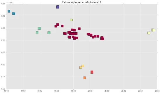
2. Extracting Region of Interest
After the stays points is detected, then we conducted the region of interest extraction using stays points. Figure 4 shows data that has been cleared from a point that does not stay points. Furthermore, the data is used to extract ROI by clustering using the DBScan algorithm.
Fig. 5 Stay points only
Fig. 6 Snippet code DBSCan clustering.
Fig. 7 The clustering results produce 9 ROI clusters
3. Modeling, Testing and Evaluation
In the training phase of the model, we implement the Gaussian HMM algorithm that is found in the library in the network. At this stage we use the parameters hmm n_components = 5, covariance_type = 'spherical', and decoder algorithm =
TABLEI EVALUATION SCORE
Evaluation Metric Score
Accuration 0.769230769231
RMSE 1.641
V. CONCLUSION
The conclusions drawn from this study are the values for parameters such as HMM n_components = 5, covariance_type = 'spherical', and decoder algorithm = 'viterbi' which produces accuration of 0.769 and RMSE 1.641 can be said to be HMM good enough in modeling data.
ACKNOWLEDGMENT
This research was supported and funded by an internal research grant (named penelitian internal) from Universitas Mercu Buana.
REFERENCES
[1] K. Zhao, S. Tarkoma, S. Liu, and H. Vo, “Urban human mobility data mining: An overview,” 2016 IEEE Int. Conf. Big Data (Big
Data), pp. 1911–1920, 2016.
[2] Y. Zheng, Y. Liu, J. Yuan, and X. Xie, “Urban computing with taxicabs,” Proc. 13th Int. Conf. Ubiquitous Comput. - UbiComp ’11, p. 89, 2011.
[3] J. Yuan, Y. Zheng, and X. Xie, “Discovering regions of different functions in a city using human mobility and POIs,” Proc. 18th
ACM SIGKDD Int. Conf. Knowl. Discov. data Min. - KDD ’12, p.
186, 2012.
[4] G. Qi, X. Li, S. Li, G. Pan, and Z. Wang, “Measuring social functions of city regions from large-scale taxi behaviors Measuring Social Functions of City Regions from Large-scale Taxi Behaviors,” no. March 2011, pp. 384–388, 2011.
[5] D. Fitrianah, A. N. Hidayanto, R. A. Zen, and A. M. Arymurthy, “APDATI: E-Fishing Logbook for Integrated Tuna Fishing Data Management,” J. Theor. Appl. Inf. Technol., vol. 75, no. 2, 2015. [6] M. Sadikin and I. Wasito, “Translation and classification algorithm
of FDA-Drugs to DOEN2011 class therapy to estimate drug-drug interaction,” in The 2nd International Conference on Information
Systems for Business Competitiveness, 2013.
[7] Y. Y. L. Huang and Y. T. D. Deng, “Improved Markov predictor in wireless networks,” IET Commun., no. April 2010, pp. 1823–1828, 2011.
[8] L. Song, D. Kotz, R. Jain, and X. He, “Evaluating next-cell predictors with extensive Wi-Fi mobility data,” IEEE Trans. Mob.
Comput., vol. 5, no. 12, pp. 1633–1648, 2006.
[9] E. G. Ravenstein, “The Laws of Migration,” J. R. Stat. Soc., vol. Vol. 48, no. 2, pp. 167–235, 1885.
[10] N. Ye, Y. Zhang, and R. Wang, “Vehicle trajectory prediction based on hidden Markov model,” KSII Trans. Internet Inf. Syst., vol. 10, no. 7, pp. 3150–3170, 2016.
[11] F. Giannotti, M. Nanni, D. Pedreschi, and F. Pinelli, “Trajectory pattern mining,” in Proceedings of the 13th ACM SIGKDD International Conference on Knowledge Discovery and Data
Mining, 2007, pp. 330–339.
[12] M. Qu, H. Zhu, J. Liu, G. Liu, and H. Xiong, “A cost-effective recommender system for taxi drivers,” in Proceedings of the 20th ACM SIGKDD International Conference on Knowledge Discovery
and Data Mining, 2014, pp. 45–54.
[13] J. Cui, F. Liu, D. Janssens, S. An, G. Wets, and M. Cools, “Detecting urban road network accessibility problems using taxi GPS data,” J Transp. Geogr., vol. 51, pp. 147–157, 2016. [14] M. A. Teixeira and G. Zaverucha, “Fuzzy Multi-Hidden Markov
Predictor in Electric Load Forecasting,” in Proceedings of
International Joint Conference on Neural Networks, 2005, pp.
1758–1763.
[15] T. Manna and I. S. Misra, “A Fast Hardware based Hidden Markov Model Predictor for Cognitive Radio,” in 2016 IEEE 6th
International Conference on Advanced Computing, 2016, pp. 752–
758.
[16] W. Mathew, R. Raposo, and B. Martins, “Predicting Future Locations with Hidden Markov Models,” 2012.
[17] “Learning to Predict Driver Route and Destination Intent - IEEE Conference Publication.” .
[18] A. Asahara, K. Maruyama, A. Sato, and K. Seto, “Pedestrian-movement Prediction Based on Mixed Markov-chain Model,” in Proceedings of the 19th ACM SIGSPATIAL International
Conference on Advances in Geographic Information Systems, 2011,
pp. 25–33.
[19] Y. Zheng, Q. Li, Y. Chen, X. Xie, and W. Ma, “Understanding Mobility Based on GPS Data,” no. 49, 2008.
[20] Y. Zheng, L. Zhang, X. Xie, and W. Ma, “Mining Interesting Locations and Travel Sequences from GPS Trajectories,” no. 49, 2009.
[21] Y. Zheng, Y. Chen, X. Xie, and W. Y. Ma, “GeoLife2.0: A location-based social networking service,” Proc. - IEEE Int. Conf.