Forecasting energy demand through a dynamic input-output model

Economics and Business Letters

4(3), 108-115, 2015

Forecasting energy demand through a dynamic input-output model

Óscar Dejuán* _{• Carmen Córcoles • Nuria Gómez • M. Ángeles Tobarra}

Department of Economics and Finance, University of Castilla-La Mancha, Spain

Received: 1 May 2015 Revised: 24 September 2015 Accepted: 18 October 2015

Abstract

This paper builds a dynamic input-output model able to forecast energy demand in different economic and legislative scenarios. Its main features are these. (1) As an input-output model embedded in a social accounting matrix that takes into account the structure of the economy and the relations between sectors (industries) and institutions (households). (2) As an applied and computable general equilibrium model it relates the system of prices and quantities. (3) As a dynamic model it considers the evolution of coefficients and energy multipliers. These are the key tools of our forecasting model and our main contribution. The simulations performed for the Spanish economy show that quantity shocks are more important than price shocks, due to the low price-elasticity of the demand for energy.

Keywords: energy demand, energy multipliers, extended input-output models JEL Classification Codes: D58, D57, E17, Q41, Q43

Nomenclature

A Matrix of technical coefficients

Ad Matrix of domestic technical coefficients

CGE Computable General Equilibrium Models

E Energy content per unit of output (A matrix or a row vector) ED Energy demand per unit of production

I Identity matrix

IOT Input-Output Tables

ME Multiplier of Energy (a matrix or arrow vector) MQ Multiplier of Total Output (a matrix or a row vector)

p Prices (a row vector)

pd Price deviation from the base value that equals one (a diagonal matrix) V Value added (a rectangular matrix)

WIOD World Input-Output Database WIOT World Input-Output tables

ya Column vector of autonomous demand (final consumption excluded)

* _{Corresponding author. E-mail: [email protected].}

 Share in output of wages and profits (a row vector)  Share in output of net taxes on energy (a row vector)  Own price elasticity (a matrix)

 Share in output of imported crude oil and natural gas  Matrix of historical trends of energy coefficients

’ Actual impact of historical trends after a change in energy prices

- - -

1. Introduction

This paper builds a dynamic input-output model able to forecast energy demand in different economic and legislative scenarios. The parameters of the model are obtained from the last Spanish input-output table (IOT) corresponding to 20101. Our simulation refers to the Spanish economy in the period 2015-2019.

The advantage of input-output analysis over macroeconomic models is that it takes into con-sideration the inter-industry connections. The energy directly demanded by the expansion of the construction industry may be quite modest. But if we add the energy demanded by firms producing the materials required to build a house, the overall demand for energy may become quite important. Even more so if we add the induced consumption of the workers directly or indirectly employed by the building sector.

Input-output models become even more useful when they are integrated in a social account-ing matrix that relates sectors (industries) with institutions (households) and when the quantity system is related to the price system. This is the essence of computable general equilibrium (CGE) models. The dominant one is based on the neoclassical theory that assumes perfect sub-stitution among factors of production in order to get full employment2. A variety of extended input-output models explore the same issues under more realistic assumptions. Dunchin (1994) and Suh & Kagawa (2005) are good examples.

In this paper we deploy the methodology advanced in Dejuán et al (2013), another extended input-output model that introduces dynamics through the alteration of the trends of energy co-efficients. The main innovations of the current paper in relation to the previous one are these:  We take the raw data from the World Input-Output Data base (WIOD) that provides input

output tables (WIOT) for 40 countries plus a closing one (rest of the world). It contains relevant and coherent data on the energy use by industries. In the future, it will make easier interregional analysis and comparisons among countries.

 The IOT has been disaggregated in order to pay due attention to the key energy producing sectors and energy consumer sectors. The information provided by the table published by the INE (Spanish statistics agency) allows us to consider 38 industries. Sector 17 in the WIOT splits into Gas (our industry 3), Electricity (4) and Water (5). Transport, the major consumer of fuels, has been disaggregated according to the infrastructure it oper-ates: rail (our industry 6), road (7), water (8) and air (9).

 Households are another big consumer of energy. We have endogenized their final con-sumption, which implies treating it as an industry. Actually, we have added two indus-tries: rural households (39) and urban households (40). For this purpose, we have used

1 _{The raw data is available for those interested in them.}

2 _{Comprehensive studies of CGE models are offered by Ginsburgh & Keyzer (2002), Kehoe, Srinivasan & Whalley}

the microdata of the “Household budget survey” (issued by EPF-INE). The criterion for splitting it up has been the size of the city (more or less than 25.000 people).

 The industry producing electricity (4) is the main provider and consumer of energy; and a very special one, indeed. Electrical companies have a variety of plants based on different technologies. They provide the electricity demanded by using fuel-based plants (coal, petrol and gas) or green ones (water, wind and solar plants). A substantial increase in the price of fossil energies is bound to change the mix of the plants operated. Even in the absence of technological improvements, this will be reflected in an alteration of the en-ergy coefficients of industry 4.For this purpose, we have consulted the information pro-vided by electrical companies.

This paper is structured in three sections apart from this introduction and the conclusions. Section 2 builds the quantity system from which we derive the energy multipliers. Section 3 deploys the cost-price system embedded in an IOT. Linking both systems (in section 4), we can track the evolution of energy demand in different scenarios corresponding to a variety of growth rates, price shocks and normative changes. Methods and data appear in sections 2 y 3. The results are in section 4. Our conclusions, in section 5.

2. The quantity system and energy multipliers

A horizontal reading of the IOT yields the quantity system. It can be presented either in an additive or in a multiplicative way:





a d

y MQ y

A I q

q y q A

· ·

·

1

 



 

 (1)

q is the column vector of total output produced in the country, total in the sense that it in-cludes intermediate and final goods. ya is the column vector of the domestic commodities

feed-ing final autonomous demand. It encompasses autonomous final consumption, private invest-ment, public expenditure on goods and services, and exports. Adis the matrix of domestic

tech-nical coefficients which has been enlarged to include induced households consumption. I is the identity matrix. The Leontief inverse (in this “augmented form”) becomes the multiplier of total output: MQ= [I-Ad]-1.

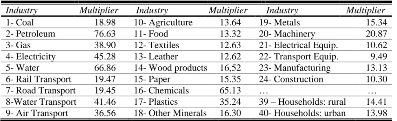
From the satellite accounts of WIOD we obtain the “energy uses”, i.e. the coal, petroleum, gas and electricity consumed by each sector. Figures appear in homogenous physical units (te-rajoules). After dividing it by the total output of each sector we obtain the energy coefficient matrix (E). After multiplying it by the Leontief inverse we get the multiplier of energy (ME), our key tool of analysis. It is a rectangular matrix with as many rows as energy sources (4) and as many columns as sectors (40). Since energy has been measured in homogeneous units, we can add up the rows and express E and ME as a row vector. The energy multipliers of table 1 and the forecast of energy demand (figure 1, section 4) appear in aggregate terms.









1 )

(t E·I Ad ·yat ME·yat

ED     (2)

chemical industry. Our model allows us to identify the amount of energy demand in each par-ticular industry dragged by the expansion of chemical products. It also makes possible a dis-aggregation of the multiplier attending to the sources of energy. In other words, we can find out the terajoules of coal, petroleum, gas and electricity associated to the expansion of chemicals or any other industry.

A final note. In our Keynesian-Sraffian input-output model for long-period predictions (1 to 5 years) changes in costs and prices may have an impact on the quantity system through the alteration of energy coefficients and multipliers. Section 3 will explore the concrete mechanisms. On the contrary, changes in the quantities produced do not affect prices because we assume constant returns to scale and a system of prices that responds to cost changes, instead of transient problems of scarcity.

3. Pricing system

A vertical reading of the IOT informs about the cost structure of industries. After dividing each column j by the value of the total output we obtain the input-output price system. It can be presented either in an additive or a multiplicative way.





· · ·

  

 

A I V p

V i A p p

(3)

p is the (row) price vector that, by construction, equals one. The input-output model auto-matically redefines the units of measurement in such a way that, in the base year, each basket of each homogenous commodity is worth one million euros. We do not know how many tons of coal are included in such a basket. We can ascertain, however, the evolution of the price of this basket and the number of baskets demanded after a supply or demand shock.

A is a 40·40 matrix of total technical coefficients (total = domestic + imported). V=++ is a rectangular matrix with as many columns as industries and three rows corresponding to the shares in total output of these three elements: (1) value added (this is  that includes wages, profits and residual rents); (2) indirect taxes on energy net of subsidies (this is ); (3) imported crude oil and natural gas demanded by refineries and gas plants (this is ). i is a unit row vector that adds the columns of V into one single row.

Table 1. Energy multipliers in the Spanish IOT-2010.

Industry Multiplier Industry Multiplier Industry Multiplier

1- Coal 18.98 10- Agriculture 13.64 19- Metals 15.34

2- Petroleum 76.63 11- Food 13.32 20- Machinery 20.87

3- Gas 38.90 12- Textiles 12.63 21- Electrical Equip. 10.62

4- Electricity 45.28 13- Leather 12.62 22- Transport Equip. 9.49

5- Water 66.86 14- Wood products 16,52 23- Manufacturing 13.13

6- Rail Transport 19.47 15- Paper 15.35 24- Construction 10.30

7- Road Transport 19.45 16- Chemicals 65.13 … …

8-Water Transport 41.46 17- Plastics 35.24 39 – Households: rural 14.41 9- Air Transport 36.56 18- Other Minerals 16.30 40- Households: urban 13.98

Table 2. Price changes after doubling the international price of crude oil and natural gas.

Industry Price Industry Price Industry Price

1- Coal 1.0529 10- Agriculture 1.0199 19- Metals 1.0280

2- Petroleum 1.6081 11- Food 1.0213 20- Machinery 1.0190

3- Gas 1.3923 12- Textiles 1.0212 21- Electrical Equip. 1.0201

4- Electricity 1.1202 13- Leather 1.0192 22- Transport Equip. 1.0200

5- Water 1.0219 14- Wood products 1.0278 23- Manufacturing 1.0192

6- Rail Transport 1.0265 15- Paper 1.0240 24- Construction 1.0122

7- Road Transport 1.0707 16- Chemicals 1.0601 …

8-Water Transport 1.0728 17- Plastics 1,0336 39 – Households: rural 1.0405 9- Air Transport 1.0836 18- Other Minerals 1.0393 40- Households: urban 1.0309 Source: Own elaboration. Initial prices are “1”. Thus, the first figure (1.0529) means an increase of 5,29%.

To illustrate the working of the price system. Imagine that the international price of crude oil and natural gas doubles at the beginning of year (1). The new price vector (p’) will be com-puted by equation [4] that provides the figures of table 1.









40 4

3 2

1 2· 2· ...

'     IA

p      (4)

We appreciate in table 2, that the impact of doubling the international price of crude oil and natural gas is mostly felt in industries 2 and 3 where petroleum is refined and gas is prepared for distribution. Their prices increase 60.81% and 39.23%. The impact is also important in the transport industries (above 7%) and Chemicals (6%). The price of the consumption basket of households increases 4.05% in rural areas and 3.09% in the cities above 25.000 inhabitants. A weighted average of the last two cells would provide an accurate computation of the consumption price index.

In general, price increases do not affect the demand for commodities because price elasticities are very low. Energy prices might be an exception because they suffer the highest impact and because energy inputs represent an important share of the cost structure. In our model, this effect is reflected in an alteration of the historical trends of energy coefficients and a new mix in the production of electricity3_.

After a relevant increase in the price of oil, electrical companies will shut down a portion of the plants burning petrol to obtain electricity and will intensify production in wind and solar plants. This will be reflected in a fall in coefficients a14, a24and a344. After this adjustment, all

firms will try to improve efficiency by saving fuels. The following equations explain the dy-namic adjustment5:

𝐴_𝑑(1)= 𝐴_𝑑(0)(𝐼 + 𝜏′)

𝐴_𝑑(2)= 𝐴_𝑑(1)(𝐼 + 𝜏′₎

…

(5)

3 _{To alter the mix, we have to assume that electrical companies have spare capacity in all their plants. This is}

clearly the case of Spain.

4 _{Other coefficients may increase, but here we are only interested in the demand for energy. Electrical companies}

provide some hints to ascertain how price changes affect the mix for generating electricity. Although our model is prepared to introduce such information, we have not used it in the simulations of section 4 that is based only in objective - quantitative data.

5 _{This maximum length of this process is five years because original input-output tables are released every five}

Table 3. Technological trends of energy coefficients.

Industry Electricity

(ind. 4)

Industry (total)

Households (total)

Coal -0.0723 0.0147 -0.0628

Petroleum -0.0704 -0.0141 -0.0471

Gas and Electricity 0.0986 0.0167 0.0420

Source: Own elaboration.

Table 4. Price elasticities.

Industry Industry

(total)

Households (total)

Coal 0.00 0.00

Petroleum -0.30 -0.08

Gas -0.0001 -0.0005

Electricity -0.03 -0.05

Source: Own elaboration comparing the literature quoted in footnote 4.

The impact of own price elasticity in the whole economy comes through the energy trends: ’=+<pd>·. Here,  is the matrix of historical trends of energy coefficients. Only cells in the four energy rows differ from zero. A negative ij shows the tendency of sector j to save energy

i year after year. We have computed them by extrapolating the tendencies of energy coefficients in the last two input – output tables corresponding to years 2005 and 2010. Matrix stands for the own-price elasticity that we take from the literature and own observations6.

Tables 3 and 4 present, in an abridged version, the trends and elasticities we have used in our simulations.

4. Simulations

Our dynamic input-output energy model allows us to figure out the evolution of energy de-mands under different scenarios. We can study the demand for energy, in the aggregate and for each specific source: coal, petroleum, gas, electricity and others. After the appropriate transfor-mations, the results may appear in physical units (terajoules, KTOES…) or in the monetary units corresponding to our IOT.

The scenarios can be related to demand shocks, supply shocks or legal changes. We can simulate the evolution of energy demand under different growth scenarios: normal, optimistic and pessimistic. We can imagine that all the elements of autonomous demand grow at the same rate or that growth is driven by a specific industry (say, construction). Supply shocks are usually associated to changes in the international price of crude oil and natural gas. Also to an increase in taxes or subsidies on specific energy inputs. The discovery of a new source of energy or a more efficient way to generate electricity; the prohibition of using a particular source due to its environmental impact, all these changes are also interpreted as supply-side shocks.

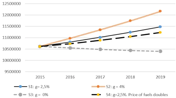
Owing to space constraints, we shall only draw a single graph with four different scenarios. The first one (S1) forecasts the total demand for energy (in terajoules) under the assumption of a moderate rate of growth of autonomous demand; g=2.5% in each year from 2015 to 20197_.

6 _{Labandeira, et al, 2006; Labanderia et al, 2012; Adeyemi & Hunt, 2007; Blázquez et al, 2013; Romero-Jordan et}

al, 2014.

The second scenario (S2) considers a boom situation with g=4%. The third scenario (S3), a period of stagnation (g=0). The fourth scenario (S4) turns back to the moderate economic ex-pansion but introduces price changes. The international price of crude oil and natural gas dou-bles.

In the case of stagnation, energy demand would fall 2% in five years due to embedded his-torical trends to save energy. In the most optimistic scenario, the demand for energy would increase by 14.6% in five years. This proves that the rate of growth of the economy is the key determinant for energy demand. For a moderate growth, energy demand would increase 8.13% in five years with constant prices and 5.80% when the prices of fuels doubles. The difference is not high because price elasticities are quite low.

Figure 1. Total energy demand under different scenarios (Spain 2015-19).

Source: Own elaboration. Units: Terajoules

5. Concluding remarks

 A dynamic input-output model, as the one deployed in this paper, is an appropriate tool for forecasting energy demand. It draws the links between: (a) different industries; (b) industries and institutions (households, in particular); and (d) prices and quantities. Price changes (after a change in technology or costs) may alter the historical trends of energy coefficient from which energy multipliers are derived.

 Economic growth is the most important determinant of energy demand. The drivers of growth may matter. An economic expansion led by industries with the highest energy-multiplier effects (transport, chemicals, construction…) would increase energy demand faster.

 Prices effects are less important because the own-price elasticity and the elasticity of sub-stitution of energy inputs are quite low.

Acknowledgements. Financial support received from Junta de Comunidades de Castilla – La Mancha / EU: PPII-2014-006-P. Jorge Zafrilla and Guadalupe Arce helped us with the computations.

References

Adeyemi, O.I. and Hunt, L.C. (2007) Modelling OECD Industrial Energy Demand: Asymmet-ric PAsymmet-rice Responses and Energy-Savings Technical Change, Energy Economics, 29, 693-709.

Blázquez, L., Boogen, N. and Filippini, M. (2013) Residential Electricity Demand in Spain: New Empirical Evidence using Aggregate Data, Energy Economics, 36, 648-657. Dejuán, Ó., López, L-A., Tobarra, M.-A., and Zafrilla, J. (2013) A Post-Keynesian AGE model

to forecast energy demand in Spain, Economic Systems Research, 25(3), 1-20.

Duchin, F. (1994) Ecological Economics, Technological Change and the Future of the Envi-ronment, Oxford: Oxford University Press.

Ginsburgh, V., and Keyzer, M. (2002) The Structure of Applied General Equilibrium Models, Cambridge, UK: Cambridge University Press.

Kehoe, T., Srinivasan, T., and Whalley, J. E. (2004) Frontiers in Applied General Equilibrium Modelling, Cambridge, UK: Cambridge University Press.

Labandeira, X., Labeaga, J.M. and Rodríguez, M. (2006) A Residential Energy Demand System for Spain, Energy Journal, 27(2), 87-112.

Labandeira, X., Labeaga, J.M. and López-Otero, X. (2012) Estimation of Elasticity Price of Electricity with Incomplete Information, Energy Economics, 34, 627-633.

Romero-Jordan, D., Peñasco, C. and del Río, P. (2014) Analysing the Determinants of House-hold Electricity Demand in Spain. An Economic Study, International Journal of Elec-trical Power & Energy Systems, 63, 950-961.