A New Generalization of the Fréchet Distribution: Properties and Application

A NEW GENERALIZATION OF THE FRÉCHET

DISTRIBUTION: PROPERTIES AND APPLICATION

Jayakumar Kuttan Pillai

Department of Statistics, University of Calicut, Kerala- 673 635, India Girish Babu Moolath1

Department of Statistics, Government Arts and Science College, Meenchanda, Kozhikode, Kerala- 673 018, India

1. INTRODUCTION

Maurice Fréchet (1878-1973), a French mathematician, introduced the Fréchet distribu-tion. This distribution is also known as the type II extreme value distribution and is a family of continuous probability distributions developed within the general extreme value theory, which deals with the stochastic behavior of the maximum and minimum of independent and identically distributed (i.i.d.) random variables (Kotz and Nadara-jah, 2000). Fréchet distribution has found to be a better model for describing stochastic phenomena, like the lifetime of components and analyzing the extreme events such as floods, earthquakes, rainfall, wind speed, sea currents, etc.

The random variableX is said to follow Fréchet distribution with the shape param-eterα >0 and the scale parameterβ >0, if the cumulative distribution function (cdf) is given by

G(x) =e−(βx)α,x>0. (1)

This distribution is equivalent to taking the reciprocal of values from a standard Weibull distribution. Extreme value theories shows that the Weibull distribution is a better model for the minimum of large number of independent positive random variables, where as, the Fréchet distribution is a better model for the maximum of a large number of random variables from a certain class of distributions, see Abbas and Tang (2015).

There have been growing interest in developing new classes of distributions for mod-elling a variety of data sets from various fields (see Jayakumar and Pillai, 1993; Pillai and Jayakumar, 1995; Jayakumar, 2003; Nadarajahet al., 2013; Jayakumar and Babu, 2018).

Gumbel (1965) studied the parameter estimation of Fréchet distribution. Nadara-jah and Kotz (2008) discussed the various sociological models based on Fréchet ran-dom variables. Several extensions of the Fréchet distribution are discussed in the lit-erature. Some of them are as follows: the exponentiated Fréchet (EF) distribution in Nadarajah and Kotz (2003), the beta Fréchet (BF) distribution in Barreto-Souzaet al. (2011), the Marshall-Olkin Fréchet (MOF) distribution in Krishna et al. (2013), the transmuted Fréchet (TF) distribution in Mahmoud and Mandouh (2013), the gamma extended Fréchet distribution in da Silva et al.(2013), the transmuted exponentiated Fréchet (TEF) distribution in Elbatalet al. (2014), the Kumaraswamy Fréchet distri-bution in Mead and Abd-Eltawab (2014), the transmuted Marshall-Olkin Fréchet dis-tribution in Afifyet al.(2015), the Kumaraswamy transmuted Marshall-Olkin Fréchet (KTMOF) distribution in Yousofet al.(2016), the Weibull Fréchet distribution in Afify et al.(2016), the beta exponential Fréchet distribution in Meadet al.(2017), the Burr-X exponentiated Fréchet (BXEF) distribution in Zayed and Butt (2017) and the generalized transmuted Fréchet (GTFr) distribution in Nofal and Ahsanullah (2019). In the present paper, we study the properties and application of a new generalization of Fréchet distri-bution, namely, exponential transmuted Fréchet (ETF) distribution.

This paper is organized as follows. In Section 2, we introduce the ETF distribution and provide its sub models. In Section 3, some structural properties of ETF distribution, including the quantile function, moments, moment generating function and order statis-tics are studied. The method of maximum likelihood is used to estimate the unknown parameters of the model and a simulation study is carried out to check the performance of the MLEs of the model parameters. These results are presented in Section 4. In Sec-tion 5, we study empirically the flexibility of ETF distribuSec-tion by using a real data set. Finally, conclusions are presented in Section 6.

2. ANEW GENERALIZATION OF THEFRÉCHET DISTRIBUTION

Even though there are many generalizations of Fréchet distribution are available in the literature, the complexity in modelling extreme values demands more flexible distribu-tions. To generate one such flexible generalization of Fréchet distribution, we consider the T-transmuted X family of Jayakumar and Babu (2017), which is defined as

F(x) =R

§

−ln

•

1−G(x)1+λG¯(x)˜ª

, (2)

whereR{t}is the cdf of the random variableT with probability density function (pdf) r(t),G(x)is the base distribution function, ¯G(x) =1−G(x)and|λ| ≤1.

e−(β

x)α,α >0,β >0,x>0. Then

F(x) =1−

•

1−e−(βx)α1+λ(1−e−( β x)α)

˜θ

,x>0. (3)

We call the distribution (3) as exponential transmuted Fréchet(ETF) distribution with parametersα >0,β >0,θ >0 and|λ| ≤1. The pdf, survival function and hazard rate function(hrf) of ETF distribution are respectively

f(x) =θαβα_x−(α+1) e−(

β

x)α(1+λ−2λe−( β x)α)

1−e−(β

x)α1+λ(1−e−(βx)α)1−θ

, (4)

S(x) =1−F(x) =

1−e−(βx)α1+λ(1−e−(βx)α)θ, (5)

and

h(x) = f(x)

1−F(x)=θαβ

α_x−(α+1) e−(

β

x)α(1+λ−2λe−( β x)α)

1−e−(βx)α1+λ(1−e−( β x)α)

. (6)

2.1. Sub models

The following are the sub models of the ETF distribution given in (3).

1. Whenλ=0, exponentiated Fréchet distribution studied in Nadarajah and Kotz (2003).

2. Whenθ=1, transmuted exponentiated Fréchet distribution studied in Elbatal et al.(2014).

3. Whenθ=1 andβ=1, transmuted Fréchet distribution studied in Mahmoud and Mandouh (2013).

4. Whenθ=1,β=1 andλ=0, Fréchet distribution.

5. Whenθ=1,β=1 andα=1, transmuted inverse exponential distribution stud-ied in Oguntunde and Adejumo (2015).

6. Whenθ=1,β=1,α=1 andλ=0, inverse exponential distribution studied in Keller and Kamath (1982).

7. Whenθ=1,β=1 andα=2, transmuted inverse Rayleigh distribution studied in Ahmadet al.(2014).

3. STRUCTURAL PROPERTIES

The shape of the pdf of ETF distribution can be described analytically by examining the roots of the equation ∂ln_∂(f_x(x))=0. It can be easily seen that lim_x→∞f(x) =0. The following result shows lim_x→0f(x) =0.

PROPOSITION1. lim_x→0f(x) =0.

PROOF. We have

lim

x→0f(x) = θαβ

α_lim

x→0 

x−(α+1)e−(βx)α

‹

lim

x→0 

1+λ−2λe−(βx)α

‹

lim

x→0 

1−e−(βx)α1+λ(1−e−(βx)α)θ−1

‹

. (7)

Sincex>0,α >0 andβ >0, we have 0≤e−(βx)α≤1.

Next, we can show that lim_x→0 x−(α+1)e−(βx)α=0.

We know that for alln∈N, lim_x→∞xne−x=0. Lettingu= (β_x)α, we have,x= β

uα1. Thusx→0 if and only ifu→ ∞and therefore,

lim

x→0 x

−(α+1)_e−(β

x)α= lim

u→∞

uα+1α _e−u

βα+1 . (8)

Now, letn∈Nsuch thatα+_α1≤n.

Then foru≥1, we haveuα+1α ≤unand thus

0≤ lim

u→∞

uα+1α _e−u

βα+1 ≤ulim→∞ un_e−u

βα+1 =0. (9)

Thus

lim

x→0 x

−(α+1)_e−(β

x)α=0. (10)

Using (10) in (7), we obtain lim_x→0f(x) =0. 2

We have

∂ ln(f(x))

∂x =

−(α+1)

x +

αβα

xα+1−

2λαβαe−(βx)α

xα+1(₁+λ₋₂λ_e−(βx)α)

−(1−θ)

αβα

xα+1

λ(2e−(βx)α−1)−1

1−e−(β

x)α1+λ(1−e−(βx)α)

=0. (11)

Here the Equation (11) may have more than one root. If x=x₀is a root, then it cor-responds to a local maximum if ∂2ln_∂(_xf2(x)) <0, a local minimum if

∂2_ln(f(x))

∂x2 >0, and a

point of inflection if ∂2ln_∂(_xf2(x))=0.

From (11) we have

f0(x) f(x) =

−(α+1) +α(β_x)α

x −

2λα(β_x)αe−(βx)α

x(1+λ−2λe−(βx)α)

−(1−θ)(

β

x)α(

α

x)e−(

β

x)α(1+λ−2λe−( β x)α)

1−e−(βx)α1+λ(1−e−( β x)α)

= s(x)

x(1+λ−2λe−(βx)α)(1−e−( β

x)α1+λ(1−e−( β x)α))

, (12)

where

s(x) = α(β

x)

α_−α−1

1+λ−2λe−(βx)α

1−e−(βx)α[1+λ(1−e−( β x)α)]

−2λα(β

x)

α_e−(βx)α1−e−( β

x)α[1+λ(1−e−( β x)α)]+

α(1−θ)(β

x)

α_e−(βx)α1+λ−2λe−( β

x)α2. (13)

Now, puty= (β_x)α_{. Sincex>0, we havey>0. Then}

s(y) =

1−e−y(1+λ) +λe−2y)

(1+λ)(y(α−1)−1)−2λe−y(y(2α−1)−1)

+α(1−θ)ye−y

1+λ−2λe−y2

= u(y)v(y) +w(y), (14)

where,u(y) =1−e−y(1+λ)+λe−2y),v(y) = (1+λ)(y(α−1)−1)−2λe−y(y(2α−1)−1) andw(y) =α(1−θ)ye−y

1+λ−2λe−y2

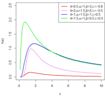
|λ| ≤1. Also note that s(y)< 0 for 0< α ≤ 1,θ >1 and |λ| ≤ 1. Hence,s(x)< 0 and f(x)is a decreasing function. In all other cases, f(x)is a unimodal function and the mode is obtained by solving the non linear Equation (11). Some possible shapes of the pdf and hrf for selected parameter values for the ETF distribution are presented in Figure 1 and Figure 2 respectively. These figures shows the flexibility of the ETF distribution. The hrf is initially increasing and then decreasing.

Figure 1 –Plot of the pdf of ETF distribution for given parameter values.

3.1. Quantile function

The following theorem gives the quantile function of ETF distribution.

THEOREM2. The ut h _{quantileφ(u)of ETF distribution is given by}

φ(u) =

  

β

−ln((1+λ)−[(1−λ)2+4λ(1−u)

1

θ_]12

2λ )

−_α1

,if|λ| ≤1andλ6=0,

β

−ln(1−(1−u)1θ)−

1

α_,ifλ=_0.

(15)

PROOF. Using (3), we have

1−

1−e−(xuβ)α₁+λ(_1−e−( β

xu)α)θ=_u

⇒ λe−2(xuβ)α₋(₁+λ)_e−( β

xu)α+₁₋(_1−u)θ1=_{0. (16)}

Putk=e−(xuβ)α_{, and this impliesx}

u=β[−ln(k)]−

1

α.

Now from (16),

λk2−(1+λ)k+

1−(1−u)θ1=_{0. (17)}

Here (17) is a quadratic equation inkand the possible root is

k=(1+λ)−

(1−λ)2_{+4λ(1−u)θ}11₂

2λ , (18)

whereλ6=0. That is

φ(u) =x_u=β

−ln (1+λ)−

(1−λ)2_+4λ(1−u)1_θ1₂ 2λ

−1_α .

Now ifλ=0, then we have

F(x) =1−[1−e−(βx)α]θ,

which implies

φ(u) =β

−ln(1−(1−u)1θ)−

1

α_.

This completes the proof. 2

Using (15) we can generate random numbers from ETF distribution. In particular whenu=0.5, the median is given by

Median=φ(0.5) =β•−ln

(1+λ)−(1−λ)2+λ22−1_θ

1 2

2λ

‹˜−1_α

The skewness and kurtosis can be defined based on the quantile function. The Galton’s skewnessSand the Moors kurtosisKare, respectively

S = Q(

6 8)−2Q(

4 8) +Q(

2 8) Q(6

8)−Q( 2 8)

,

K = Q( 7 8)−Q(

5 8) +Q(

3 8)−Q(

1 8) Q(6₈)−Q(2₈) .

ForS=0, the distribution is symmetric, whenS>0 (orS<0), the distribution is right (or left) skewed. As the value of kurtosis increases, the tail of the distribution becomes heavier. Table 1, shows the changes of skewness and kurtosis for various parameter values of the ETF distribution. Here we can observe that the skewness and kurtosis of the ETF distribution, (i) decreases asαincreases andβ,θ,λare fixed , (ii) decreases asθ increases andα,β,λare fixed , (iii) remains constant asβincreases andα,θ,λare fixed, and (iv) increasing when−1≤λ <0 and decreasing when 0≤λ≤1, for fixedα,βand θ.

TABLE 1

Measures of skewness and kurtosis of ETF distribution for given parameter values.

α β θ λ Skewness (S) Kurtosis (K)

0.5 0.5 0.5 -1.0 0.910 16.730

-0.5 0.913 16.815

0.0 0.911 16.730

0.5 0.885 14.962

1.0 0.729 4.529

1.0 1.0 1.0 1.0 0.330 1.599

1.5 0.260 1.460

2.0 0.230 1.397

5.0 0.144 1.292

1.0 0.5 1.0 0.9 0.351 1.681

1.0 0.351 1.681

2.0 0.351 1.681

5.0 0.351 1.681

0.5 0.5 0.5 0.9 0.778 6.857

1.0 0.527 2.680

2.0 0.350 1.788

3.2. Moments

The following theorem gives therth_{raw moment of the ETF distribution.}

THEOREM3. If X has the ETF distribution with|λ| ≤1, then the rt h _{raw moment is}

given by

µ0

r(x) =

∞

X

j=0

∞

X

k=0

∞

X

l=0

(−1)j+lθβr(1+λ) _θ −1 j j k k l

Γ(₁₋ r

α)

(1+j+l)1−r_α

−

∞

X

j=0

∞

X

k=0

∞

X

l=0

2(−1)j+l_θβr_λk+1 _θ −1 j j k k l

Γ(₁₋r

α)

(2+j+l)1−αr

. (20)

PROOF. We have

µ0

r(x) =E(Xr) =

Z∞ 0

xrf(x)d x

=

Z∞ 0

θαβα_xr−(α+1)_e−(βx)α[1+λ−2λe−( β x)α]

• 1−e−(β

x)α1+λ(1−e−(βx)α)

˜1−θ d x. (21)

Lett= (β_x)α, thenx=βt−(1α)_{. Therefore (21) becomes}

µ0

r(x) =

Z∞ 0

θβr_t−(r

α)_e−t[₁+λ₋₂λ_e−t]

•

1−e−t

1+λ(1−e−t₎˜

1−θ d t. (22)

Using the expansion(1−z)θ−1₌P∞

j=0(−1)j θ− 1

j

zj_{, we have}

•

1−e−t

1+λ(1−e−t)˜θ− 1

=X∞

j=0

(−1)j _θ

−1

j

•

e−t

1+λ(1−e−t)˜

j

Thus

µ0

r(x) =

Z∞ 0

θβr_t−(r

α)_e−t₁+λ₋₂λ_e−t ∞

X

j=0

(−1)j

_θ

−1

j

e−t

1+λ(1−e−t₎j

d t

=

Z∞ 0

θβr_t−(r

α)_e−t ₁+λ ∞

X

j=0

(−1)j _θ

−1

j

e−t

1+λ(1−e−t)j

d t

−

Z∞ 0

2θλβrt−(αr)_e−2t

∞

X

j=0

(−1)j _θ

−1

j

e−t

1+λ(1−e−t)j

d t

= I₁−I₂, (23)

where

I₁ =

Z∞ 0

θβr_t−(r

α)_e−t(₁+λ)

∞

X

j=0

(−1)j _θ

−1

j

•

e−t

1+λ(1−e−t)˜

j

d t

= Z∞

0

θ(1+λ)βrt−(αr)

∞

X

j=0

(−1)j _θ

−1

j

e−(1+j)t ∞

X

k=0 _j

k

λ(1−e−t)k

d t

= X∞

j=0

∞

X

k=0

∞

X

l=0

θ(1+λ)λkβr(−1)j+l _θ −1 j j k k l Z∞ 0

t(αr)_e−(1+j+l)t _{d t}

= X∞

j=0

∞

X

k=0

∞

X

l=0

(−1)j+lθ(1+λ)βr _θ −1 j j k k l

Γ(₁₋r

α)

Similarly

I₂ =

Z∞ 0

2θλβrt−(αr)_e−2t ∞

X

j=0

(−1)j _θ

−1

j

•

e−t

1+λ(1−e−t)˜

j

d t

= X∞

j=0

∞

X

k=0

∞

X

l=0

2(−1)j+lθβrλk+1 _θ −1 j j k k l

Γ(₁₋ r

α)

(2+j+l)1−_αr. (25)

Substituting (24) and (25) in (23) we get the result (20).

This completes the proof. 2

3.3. Moment generating function

The moment generating function (mgf) of the ETF distribution is given in the following theorem.

THEOREM4. If X has the ETF distribution with|λ| ≤1, then the mgf is given by

M_X(t) = ∞

X

r=0 tr

r!µ 0

r(x), (26)

where

µ0

r(x) =

∞

X

j=0

∞

X

k=0

∞

X

l=0

(−1)j+lθβr(1+λ) _θ −1 j j k k l

Γ(₁₋ r

α)

(1+j+l)1−r_α

−

∞

X

j=0

∞

X

k=0

∞

X

l=0

2(−1)j+lθβrλk+1 _θ −1 j j k k l

Γ(₁₋r

α)

(2+j+l)1−αr

.

Proof follows easily.

3.4. Order statistics

kth_{order statistic, sayZ=X}

(k), the pdf and cdf are respectively given by

f_Z(z) = n! (k−1)!(n−k)!F

k−1_{(z)[1−F(z)]}n−k_f(z)

= n!

(k−1)!(n−k)! •

θαβα_z−(α+1)_e−(βz)α(1+λ−2λe−( β z)α)

˜

• 1−

1−e−(βz)α1+λ(1−e−( β z)α)θ

˜k−1

•

1−e−(βz)α1+λ(1−e−( β z)α)

˜θ(n−k+1)−1

, (27)

and

F_Z(z) =

n

X

j=k

n j

Fj(z)[1−F(z)]n−j

= Xn

j=k

n j

• 1−

1−e−(βz)α[1+λ(1−e−(βz)α)]θ

˜j

•

1−e−(βz)α[1+λ(1−e−( β z)α)]

˜θ(n−j)

. (28)

The pdf of minimum is

f_X

(1)(z) = nθαβ

α_z−(α+1)_e−(β

z)α(1+λ−2λe−(βz)α)

•

1−e−(βz)α1+λ(1−e−( β

z)α)

˜nθ−1

, (29)

and the pdf of the maximum is

f_X

(n)(z) = n

•

θαβα_z−(α+1)_e−(βz)α(1+λ−2λe−( β z)α)

˜

• 1−

1−e−(βz)α1+λ(1−e−(βz)α)θ

˜n−1

•

1−e−(βz)α1+λ(1−e−( β

z)α)

˜θ−1

. (30)

4. MAXIMUM LIKELIHOOD ESTIMATES OF THE PARAMETERS

ETF(α,β,θ,λ)distribution. The likelihood functionLis given by

L=θn_αn_βnαe

−Pn

i=1(xiβ)αQn

i=1x

−(α+1)

i

Qn

i=1(1+λ−2λe

−(_xiβ)α )

Qn i=1

•

1−e−(xiβ)α

1+λ(1−e−(xiβ)α) ˜1−θ

. (31)

The log-likelihood function can be written as

log(L) = nlog(θ) +nlog(α) +nαlog(β)−βαXn

i=1 x−α

i

−(α+1)

n

X

i=1

log(x_i) +

n

X

i=1

log(1+λ−2λe−(xiβ)α)

+(θ−1)

n

X

i=1 log

•

1−e−(xiβ)α₁+λ(_1−e−( β xi)α)

˜

. (32)

The MLE, ˆe = (αˆ, ˆβ, ˆθ, ˆλ)T _{ofe= (α,β,θ,λ)}T _{is obtained by maximizing the}

log-likelihood function. We have

∂ log(L)

∂ α =

n

α+nlog(β)−βαlog(β)

n

X

i=1

x−_iα+βα

n

X

i=1

x_i−αlog(x_i)

−

n

X

i=1

log(x_i) +2λ

n

X

i=1

(β_x i)

α_log(β

x_i)e−(

β x)α

1+λ−2λe−(βx)α

+(θ−1)

n

X

i=1

(β_x i)

α_log(β

xi)e

−(βx)α[1+λ−2λe−( β x)α]

1−e−(βxi)α₁+λ(_1−e−( β xi)α)

=0, (33)

∂ log(L)

∂ β =

nα β − α β n X

i=1

(β x_i)

α₊2λα

β

n

X

i=1

(β_x i)

α_e−(β xi)α

1+λ−2λe−(β x)α

+(θ−1)

n

X

i=1

α β(βxi)

α_e−(_xiβ)α

1+λ−2λe−(β x)α

1−e−(βxi)α₁+λ(_1−e−( β xi)α)

=0, (34)

∂ log(L)

∂ θ =

n

θ+

n

X

i=1 log

•

1−e−(βxi)α₁+λ(_1−e−( β xi)α)

˜

and

∂ log(L)

∂ λ =

n

X

i=1

1−2e−(xiβ)α

1+λ−2λe−(βxi)α

−

n

X

i=1

(θ−1)e−(xiβ)α(_1−e−( β xi)α)

1−e−(βxi)α₁+λ(_1−e−( β xi)α)

=0. (36)

These equations cannot be solved analytically and the R software can be used to solve them numerically. The normal approximation of the MLE ofecan be used for con-structing the approximate confidence limits and for testing hypothesis on the parame-tersα,β,θandλ. Under the conditions that are fulfilled for parameters in the interior of the parameter space, we havepn(ˆe−e)∼N(0,K−1

e ), where∼means approximately

distributed andK_e is the unit expected information matrix. The asymptotic behavior is valid ifK_e=lim_n→∞n−1_I

n(e), whereIn(e)is the observed information matrix. The

Fisher’s information matrix is given by

I_X(e) =             

−E(∂2_{∂ α}l n(2L)) −E( ∂2_{l n(L)}

∂ α∂ β) −E(∂ 2_{l n(L)}

∂ α∂ θ ) −E(∂ 2_{l n(L)} ∂ α∂ λ )

−E(∂_{∂ β∂ α}2l n(L)) −E(∂2_{∂ β}l n(2L)) −E( ∂2_{l n(L)}

∂ β∂ θ) −E(∂ 2_{l n(L)} ∂ β∂ λ)

−E(∂_{∂ θ∂ α}2l n(L)) −E(∂_{∂ θ∂ β}2l n(L)) −E(∂2_∂l n2_θ(L)) −E( ∂2_{l n(L)}

∂ θ∂ λ )

−E(∂_{∂ λ∂ α}2l n(L)) −E(∂_{∂ λ∂ β}2l n(L)) −E(∂_{∂ λ∂ θ}2l n(L)) −E(∂2_∂l n2_λ(L))

             . (37)

Here, the ETF(α,β,θ,λ)distribution satisfies the regularity conditions which are full filled for the parameters in the interior of the parameter space, but not on the bound-ary. Hence, the vector ˆeis consistent and asymptotically normal. That is,p

I_X(e)[ˆe−e] converges in distribution to multivariate normal with zero mean vector and identity co-variance matrix. The Fisher’s information matrix can be computed using the approxi-mation,

I_X(ˆe)≈

            

−∂2_{∂ α}l n(2L)|ˆe −∂

2_{l n(L)} ∂ α∂ β |ˆe −∂

2_{l n(L)} ∂ α∂ θ |ˆe −∂

2_{l n(L)} ∂ α∂ λ |ˆe

−∂_{∂ β∂ α}2l n(L)|ˆe −∂

2_{l n(L)} ∂2_β |ˆe −∂

2_{l n(L)} ∂ β∂ θ |ˆe −∂

2_{l n(L)} ∂ β∂ λ|ˆe

−∂_{∂ θ∂ α}2l n(L)|ˆe −∂

2_{l n(L)} ∂ θ∂ β |ˆe −∂

2_{l n(L)} ∂2_θ |ˆe −∂

2_{l n(L)} ∂ θ∂ λ |ˆe

−∂_{∂ λ∂ α}2l n(L)|ˆe −∂

2_{l n(L)} ∂ λ∂ β|ˆe −∂

2_{l n(L)} ∂ λ∂ θ |ˆe −∂

2_{l n(L)} ∂2_λ |ˆe

We compute the maximized unrestricted and restricted log-likelihood ratio (LR) test statistic for testing on some ETF sub models. We can use the LR test statistic to check whether the ETF distribution for a given data set is statistically superior to the sub mod-els. For example,H₀:θ=1 versusH₁:θ6=1 is equivalent to compare the ETF distribu-tion and transmuted exponentiated Fréchet (TGF) distribudistribu-tion and the LR test statistic reduce toω=2(l(αˆ, ˆβ, ˆθ, ˆλ)−l(αˆ0

, ˆβ0 , 1, ˆλ0

)), where(αˆ, ˆβ, ˆθ, ˆλ)and(αˆ0 , ˆβ0

, ˆλ0

)are the MLEs underH₁andH₀, respectively. The test statisticωis asymptotically (asn→ ∞) distributed asχ2

(k), wherekis the length of the parameter vector of interest. The LR test rejectsH₀ifω > χ2

(k,α)whereχ(2k,α)denotes the upper 100(1−α)% quantile of theχ(2k) distribution.

4.1. Simulation study

This section explains the performance of the MLEs of the model parameters of the ETF distribution using Monte Carlo simulation for various sample sizes and for selected pa-rameter values. The algorithm for the simulation study is given below.

Step 1. Input the value of replication (N).

Step 2. Specify the sample sizenand the values of the parametersα,β,θandλ.

Step 3. Generateu_i∼Uniform(0, 1),i=1, 2, ...,n.

Step 4. Obtain the random observations from the ETF distribution using (15).

Step 5. Compute the MLEs of the four parameters.

Step 6. Repeat steps 3 to 5, N times.

Step 7. Compute the parameter estimate, standard error of estimate, average bias, mean square error (MSE) and coverage probability (CP) for each parameter.

Here the expected value of the estimator isE(ˆe) =_N1PN

i=1ˆei, with

E(SE(ˆe)) = v u t1

N

PN i=1



−∂2_∂log_e2(L)

i

‹ ,

Average Bias=_N1 PN

i=1(ˆei−e), MSE(ˆe) =

1

N

PN

i=1(ˆei−e)2and

Coverage Probability=Probability ofe_i∈



ˆe_i±1.96r−∂2_∂log_e2(L)

i

‹ .

error, average bias, MSE and CP are computed and presented in Table 2. From Table 2, it can be seen that, as sample size increases the estimates of bias and MSE are decreasing. Also note that the CP values are quite close to the 95% nominal level.

TABLE 2

The parameter estimate, standard error, average bias, MSE and CP for given parameter values.

Parameter(e) Samples(n) E(ˆe)(E(SE(ˆe))) Average bias MSE CP

α=0.5

50 100 200 500 0.538(0.010) 0.490(0.008) 0.499(0.005) 0.505(0.003) 0.027 -0.018 -0.003 0.005 0.002 0.002 0.001 0.001 85.2 89.4 90.8 94.3

β=1.5

50 100 200 500 1.715(0.060) 1.638(0.051) 1.476(0.044) 1.494(0.035) 0.204 0.146 -0.034 -0.006 0.051 0.020 0.002 0.001 82.3 85.3 89.1 93.1

θ=3

50 100 200 500 3.161(0.054) 3.136(0.067) 3.083(0.036) 3.053(0.077) 0.146 0.125 0.068 0.043 0.036 0.017 0.007 0.003 87.5 90.9 92.2 94.4

λ=−0.9

50 100 200 500 -0.602(0.011) -0.650(0.010) -0.707(0.009) -0.761(0.008) 0.318 0.280 0.179 0.122 0.079 0.063 0.037 0.019 83.8 87.3 89.8 91.2

α=1.5

50 100 200 500 1.942(0.072) 1.781(0.059) 1.713(0.052) 1.668(0.033) 0.442 0.137 0.112 0.109 0.037 0.029 0.011 0.007 86.7 88.9 90.2 92.8

β=0.5

50 100 200 500 0.327(0.011) 0.399(0.008) 0.429(0.008) 0.473(0.007) -0.162 -0.148 -0.093 -0.041 0.017 0.011 0.009 0.004 89.3 90.1 91.7 93.4

θ=1

50 100 200 500 1.319(0.218) 1.212(0.173) 1.114(0.109) 1.105(0.098) 0.297 0.201 0.183 0.105 0.091 0.062 0.044 0.039 91.6 92.5 93.6 93.9

λ=0.5

50 100 200 500 0.869(0.028) 0.814(0.022) 0.722(0.019) 0.631(0.017) 0.342 0.299 0.241 0.183 0.018 0.017 0.014 0.011 84.8 86.1 86.9 88.7

5. DATA APPLICATION

patients (Lee and Wang, 2003). The data are as follows:

0.080 0.200 0.400 0.500 0.510 0.810 0.900 1.050 1.190 1.260 1.350 1.400 1.460 1.760 2.020 2.020 2.070 2.090 2.230 2.260 2.460 2.540 2.620 2.640 2.690 2.690 2.750 2.830 2.870 3.020 3.250 3.310 3.360 3.360 3.480 3.520 3.570 3.640 3.700 3.820 3.880 4.180 4.230 4.260 4.330 4.340 4.400 4.500 4.510 4.870 4.980 5.060 5.090 5.170 5.320 5.320 5.340 5.410 5.410 5.490 5.620 5.710 5.850 6.250 6.540 6.760 6.930 6.940 6.970 7.090 7.260 7.280 7.320 7.390 7.590 7.620 7.630 7.660 7.870 7.930 8.260 8.370 8.530 8.650 8.660 9.020 9.220 9.470 9.740 10.06 10.34 10.66 10.75 11.25 11.64 11.79 11.98 12.02 12.03 12.07 12.63 13.11 13.29 13.80 14.24 14.76 14.77 14.83 15.96 16.62 17.12 17.14 17.36 18.10 19.13 20.28 21.73 22.69 23.63 25.74 25.82 26.31 32.15 34.26 36.66 43.01 46.12 79.05.

The fit of the data set is compared with the sub models of the ETF distribution and the competitive models namely, Kumaraswamy Fréchet(KF) distribution, transmuted Marshall-Olkin Fréchet(TMOF) distribution and Weibull Fréchet(WF) distribution. The pdfs of these distributions are, respectively:

KF: f(x) =abβθβx−β−a_e−a(θx)β(1−e−a( θ

x)β)b−1,x>0;

TMOF:f(x) =αβσβx−β−1e−( σ x)β

(α+(1−α)e−a(θx)β)2

•

1+λ− 2λe−a(

θ x)β

α+(1−α)e−a(θx)β

˜ ,x>0;

WF: f(x) =abβαβx−β−1e−b(αx)β(1−e−b(αx)β)−b−1e−a(e−b( α x)β₋1)−b

,x>0.

Descriptive statistics of the data set are given in Table 3.

TABLE 3

Descriptive statistics of the remission times (in months) of 128 bladder cancer patients. Descriptive Statistics

Sample size(n) 128.000

Mean 9.366

SD 10.508

Minimum 0.080

Maximum 79.050

Skewness 3.326

Kurtosis 16.154

Figure 3 –Empirical TTT plot of the data set.

The estimates of the unknown parameters are obtained by the maximum-likelihood estimation method. To compare the distributions we consider the criteria like, Kol-mogorov -Smirnov (K-S) statistic (the distance between the empirical cdf’s and the fit-ted cdf’s), Akaike information criterion (AIC), Bayesian information criterion (BIC), corrected Akaike information criterion (CAIC), Cramér - von Mises criterion (W*) and Anderson - Darling criterion (A*). The best distribution corresponds to lower -logL, AIC, BIC, CAIC, K-S distance, A*, W* statistics and higher p value. Here, AIC=−2 logL+2k, CAIC=−2 logL+ (_n−2kn_k−1)and BIC=−2 logL+klogn whereL is the likelihood function evaluated at the maximum likelihood estimates,kis the num-ber of parameters andnis the sample size. The K-S distance,D_n=sup_x|F(x)−F_n(x)|, where,F_n(x)is the empirical distribution function. LetF(x;e)be the cdf and the form ofF is known buteis unknown. Then the statistics W* and A* are computed as follows: (i) computeξi=F(xi; ˆe)where thexi’s are in ascending order; (ii) computexi=φ−1(ξi),

whereφ(.)is the normal cdf andφ−1_{(.)is its inverse; (iii) computey}

i=φ((xi−¯x)/sx),

where ¯x=_n1Pn

i=1xiandsx2=

1

n−1 Pn

i=1(xi−¯x)2; (iv) calculate

W2=

n

X

i=1 

y_i−2i−1

2n

‹2

+ 1

12n

and

A=−n− 1

n

n

X 1=1 •

(2i−1)log(y_i) + (2n+1−2i)log(1−y_i)

(v)W∗_=W2₍₁₊0.5

n)andA∗=A2(1+

0.75

n +

2.25

n2), see Chen and Balakrishnan (1995).

TABLE 4

The parameter estimates with standard error (SE) and -log(likelihood).

Model ML estimates(SE) -log L

F αˆ=0.752(0.040), ˆβ=3.256(0.410) 444.001

TMOF αˆ=2.711(0.630), ˆβ=0.795(0.090), ˆ

σ=0.445(0.150), ˆλ=−0.999(0.030) 438.799

TGF αˆ=0.836_ˆ(0.050), ˆβ=1.707(0.220),

λ=−0.856(0.090) 436.678

KF aˆ_ˆ=1.969(0.210), ˆb=54.159(19.650),

β=0.241(0.030), ˆθ=168.832(16.430) 412.473

WF αˆ=118.595(34.540), ˆβ=0.209(0.010), ˆ

a=36.738(7.850), ˆb=2.377(0.100) 411.511

ETF α_ˆˆ=0.323(0.040), ˆβ=53.030(37.330),

θ=31.519(17.930), ˆλ=−0.966(0.030) 410.833

TABLE 5 Goodness of fit statistics.

Model AIC CAIC BIC A* W* K-S p-value

F 892.002 892.098 897.706 6.121 0.980 0.427 2.2x10−16 TMOF 885.599 885.924 897.007 6.859 1.146 0.155 0.004

TGF 879.356 879.549 887.912 4.588 0.698 0.124 0.039

KF 832.946 833.271 844.354 0.591 0.085 0.053 0.865

WF 831.023 831.348 842.431 0.411 0.063 0.055 0.839

ETF 829.666 829.991 841.074 0.236 0.030 0.039 0.989

The values in Table 4 and Table 5 show that the ETF distribution leads to better fit compared to the other five models. Figure 4, show the fitted cdfs with the empirical distribution of the data set.

Figure 4 –Fitted cdf plots and the empirical distribution of the data set.

6. CONCLUSION

In this paper, we propose a new four-parameter model named as the exponential trans-muted Fréchet (ETF) distribution, which extends the Fréchet distribution. We study some of its mathematical and statistical properties. The expressions for the quantile function, moments, moment generating function and order statistics are derived. The model parameters are estimated using maximum likelihood estimation method and a simulation study to illustrate the performance of the method is presented. The new distribution was applied to a real data set to show its flexibility for data modelling.

ACKNOWLEDGEMENTS

REFERENCES

K. ABBAS, Y. TANG(2015).Analysis of Fréchet distribution using reference priors. Com-munications in Statistics-Theory and Methods, 44, pp. 2945–2956.

A. Z. AFIFY, G. G. HAMEDANI, I. GHOSH, M. E. MEAD(2015). The transmuted Marshall-Olkin Fréchet distribution: Properties and applications. International Journal of Statistics and Probability, 4, pp. 132–148.

A. Z. AFIFY, H. M. YOUSOF, G. M. CORDEIRO, E. M. M. ORTEGA, Z. M. NOFAL (2016).The Weibull Fréchet distribution and its applications. Journal of Applied Statis-tics, 43, pp. 2608–2626.

A. AHMAD, S. P. AHMAD, A. AHMED (2014). Transmuted inverse Rayleigh

distribu-tion: A generalization of the inverse Rayleigh distribution. Mathematical Theory and Modeling, 4, pp. 90–98.

W. BARRETO-SOUZA, G. M. CORDEIRO, A. B. SIMAS(2011). Some results for beta Fréchet distribution. Communications in Statistics-Theory and Methods, 40, pp. 798– 811.

G. CHEN, N. BALAKRISHNAN(1995).A general purpose approximate goodness-of-fit test. Journal of Quality Technology, 27, pp. 154–161.

R. V.DASILVA, T. A. N.DEANDRADE, D. B. M. MACIEL, R. P. S. CAMPOS, G. M. CORDEIRO(2013). A new lifetime model: The gamma extended Fréchet distribution. Journal of Statistical Theory and Applications, 12, pp. 39–54.

I. ELBATAL, G. ASHA, A. V. RAJA(2014). Transmuted exponentiated Fréchet distribu-tion: Properties and applications. Journal of Statistics Applications and Probability, 3, pp. 379–394.

E. J. GUMBEL(1965). A quick estimation of the parameters in Fréchet’s distribution. Re-view of the International Statistical Institute, 33, pp. 349–363.

K. JAYAKUMAR(2003). Mittag-Leffler process. Mathematical and Computer Modelling, 37, pp. 1427–1434.

K. JAYAKUMAR, M. G. BABU(2017).T-transmuted X family of distributions. Statistica, 77, pp. 251–276.

K. JAYAKUMAR, M. G. BABU(2018). Discrete Weibull geometric distribution and its

properties. Communications in Statistics-Theory and Methods, 47, pp. 1767–1783.

A. Z. KELLER, A. R. KAMATH(1982). Reliability analysis of CNC machine tools. Relia-bility Engineering, 3, pp. 449–473.

S. KOTZ, S. NADARAJAH(2000).Extreme Value Distributions Theory and Applications. World Scientific, London.

E. KRISHNA, K. K. JOSE, T. ALICE, M. M. RISTI ´C(2013). The Marshall-Olkin Fréchet

distribution. Communications in Statistics-Theory and Methods, 42, pp. 4091–4107.

E. T. LEE, J. WANG(2003). Statistical Methods for Survival Data Analysis. John Wiley and Sons, New York.

M. R. MAHMOUD, R. M. MANDOUH(2013). On the transmuted Fréchet distribution. Journal of Applied Sciences Research, 9, pp. 5553–5561.

M. E. MEAD, A. R. ABD-ELTAWAB(2014).A note on Kumaraswamy Fréchet distribution. Australian Journal of Basic and Applied Sciences, 8, pp. 294–300.

M. E. MEAD, A. Z. AFIFY, G. G. HAMEDANI, I. GHOSH(2017). The beta exponential

Fréchet distribution with applications. Austrian Journal of Statistics, 46, pp. 41–63.

S. NADARAJAH, K. JAYAKUMAR, M. M. RISTI ´C(2013).A new family of lifetime models. Journal of Statistical Computation and Simulation, 83, pp. 1389–1404.

S. NADARAJAH, S. KOTZ(2003).The exponentiated Fréchet distribution. InterStat Elec-tronic Journal, 31, pp. 1–7.

S. NADARAJAH, S. KOTZ(2008).Sociological models based on Fréchet random variables. Quality & Quantity, 42, pp. 89–95.

Z. M. NOFAL, M. AHSANULLAH(2019). A new extension of the Fréchet distribution:

Properties and its characterization. Communications in Statistics-Theory and Meth-ods, 48, pp. 2267–2285.

P. E. OGUNTUNDE, A. O. ADEJUMO(2015). The transmuted inverse exponential

dis-tribution. International Journal of Advanced Statistics and Probability, 3, pp. 1–7.

R. N. PILLAI, K. JAYAKUMAR(1995). Discrete Mittag-Leffler distributions. Statistics & Probability Letters, 23, pp. 271–274.

V. G. VODA(1972). On the inverse Rayleigh distributed random variable. Reports of Statistical Application Research, 19, pp. 13–21.

H. M. YOUSOF, A. Z. AFIFY, A. N. EBRAHEIM, G. G. HAMEDANI, N. S. BUTT(2016).

M. ZAYED, N. S. BUTT(2017). The extended Fréchet distribution: Properties and appli-cations. Pakistan Journal of Statistics and Operation Research, 13, pp. 529–543.

SUMMARY

A new generalization of the Fréchet distribution is introduced and studied. Its structural proper-ties including the quantile function, random number generation, moments, moment generating function and order statistics are investigated. The unknown parameters of the model are estimated using maximum likelihood estimation method and a simulation study is carried out to check the performance of the method. The new model is applied to a real data set to prove empirically its flexibility.