Federal Reserve Bank of Dallas
Globalization and Monetary Policy Institute
Working Paper No. 207
http://www.dallasfed.org/assets/documents/institute/wpapers/2014/0207.pdf
Can Interest Rate Factors Explain Exchange Rate Fluctuations?
*Julieta Yung
Federal Reserve Bank of Dallas
October 2014
Abstract
This paper explores whether interest rate factors, derived from the yield curve, can explain
exchange rate fluctuations at different horizons. Using a dynamic term structure model
under no-arbitrage, exchange rates are modeled as the ratio of two countries’ stochastic
discount factors. Key to this framework is that factors are observable, which allows the
model to be estimated by Maximum Likelihood. Results show that interest rate factors can
explain half of the variation in one-year exchange rates and up to ninety percent of five-year
movements, for free-floating currencies from 1999 to 2014. These findings suggest that yield
curves contain important information for modeling exchange rate dynamics, particularly at
longer horizons.
JEL codes: G15, F31, E43
*
Julieta Yung, Federal Reserve Bank of Dallas, Research Department, 2200 N. Pearl Street, Dallas, TX 75201. 214 922-5443. [email protected]. I am grateful to Tom Cosimano, Jun Ma, Mark Wohar, and many others for helpful comments and suggestions. This paper also benefited from comments made by the participants at the Macroeconomics Seminar and the Mathematical Finance Research Group at the University of Notre Dame. The views in this paper are those of the author and do not necessarily reflect the views of the Federal Reserve Bank of Dallas or the Federal Reserve System.
1
Introduction
The motivation for this paper arises from the idea that a few common factors drive most of the movement in asset prices. Investors deciding how to allocate their wealth consider portfolios with different risk profiles, assets with various time horizons, and investment opportunities in different countries. We can therefore think of a unique pricing mechanism that simultaneously determines prices of assets, such as bonds and exchange rates, given a limited set of information available at any point in time. In this paper, I explore whether interest rate factors extracted from the yield curve can explain exchange rate fluctuations across a number of different horizons.
Exchange rates are modeled as the ratio of two countries’ stochastic discount factors, derived from a dynamic term structure model with observable interest rate factors. In this context, exchange rate movements are driven by three components: (i) the interest rate differential, which is linear in the factors, (ii) a nonlinear risk premium that varies throughout time, and (iii) the difference in shocks to the prices of risk. The interest rate factors driving exchange rate movements, the level, slope, and curvature, are principal components from the yield curve that capture over 99% of cross-sectional variation within a country. This paper contributes to the international and macro-finance literature by modeling movements in the exchange rate from one month to five years, through a dynamic no-arbitrage term structure model, using only factors from the yield curve. The results suggest that yield curves contain important information for modeling exchange rate dynamics during the 1999-2014 period, particularly at longer horizons. For example, three observable interest rate factors from each country can explain about half of the variation in one-year exchange rates for countries with free-floating currencies relative to the U.S. dollar: Australia (57%), Canada (45%), Japan (61%), Norway (49%), Sweden (70%), Switzerland (42%), and the U.K. (61%). As the horizon increases, between 55% (Swiss franc) and 92% (British pound) of the five-year exchange rate fluctuations are accounted for by these observable factors alone. Results are robust to correcting for small-sample bias with different simulation-based bootstrapping methods and adjusting for potential heteroskedasticity in the error term, suggesting that interest rate factors can better explain fluctuations in exchange rates at longer terms. These findings are in line with work by Mark (1995), who finds that exchange rate fluctuations become more predictable at longer horizons. Key to my paper is that factors are observable, which allows the no-arbitrage term structure model to be estimated by Maximum Likelihood, as in Joslin, Singleton, and Zhu (2011).
The main driver of exchange rate fluctuations in this model is a time-varying risk premium, nonlinear in the factors, derived from the countries’ stochastic discount factors. This component is consistent with the Fama (1984) conditions: it is negatively correlated with the interest rate differential and exhibits a signifi-cantly higher volatility. I therefore study the model-implied risk premium in the context of the uncovered
interest parity condition, which links expected exchange rate movements to the interest rate differential be-tween two countries with a coefficient of one. The puzzle in this literature arises when the coefficient is not only different from one, but also negative. I project log exchange rate changes in the data onto the interest rate differential and the risk premium components implied by the model. After including the risk premium, the coefficient of the interest rate differential becomes consistently positive (except for Sweden at the one-and three-month horizons), approaches one, one-and is statistically significant at longer horizons. The coefficient of the risk premium is always positive, approaches one, and is statistically significant for all currencies at horizons greater than one month. This suggests that the risk premium implied by the model is not only consistent with the theory, but also important in explaining exchange rate dynamics.
The ability of interest rate factors to explain cross-sectional variation in the yield curve decreases with the number of factors. The yield curve’s third factor, or curvature, can explain less than 1% of interest rate movements for most countries. Interestingly, the model finds that the curvature factor significantly contributes to explaining exchange rate fluctuations despite its low explanatory power for the cross-section of interest rates. For example, a model with two factors (level and slope) can only account for 28% of variation in the one-year Japanese yen, compared to 61% with a three-factor model, and this is true for most currencies studied. One exception is the Canadian dollar, since one-year fluctuations are well captured by two factors alone, and incorporating a curvature factor only improves the fit of the model from 42% to 45%. The findings in this paper are not driven by the U.S. dollar or any one country in particular. I explore exchange rates in terms of the British pound, instead of the U.S. dollar, which implies U.K. interest rate factors are extracted from the yield curve. In general, results are very similar regardless of the chosen base, and the fit of the model improves at longer horizons, consistent with the baseline results. For some countries, for example Canada, modeling one-year exchange rate fluctuations with respect to the British pound significantly improves the model’s fit from 45% to 64%. This suggests that the U.S. term structure does not contain more information on exchange rate movements than the U.K. Regardless of the country base, exchange rate fluctuations are well captured in the long run by the same factors that explain cross-sectional interest rate variation.
My model also allows one to explore a variety of questions; for example, which countries under the euro can better explain exchange rate movements? I extract interest rate factors from countries under the euro regime: Austria, Belgium, Finland, France, Germany, Ireland, Italy, the Netherlands, Portugal, and Spain. In the baseline framework, each country’s interest rate factors capture the dynamics of the exchange rate at different horizons, relative to the U.S. dollar. In the case of the euro, however, individual countries exhibit very different yield curves, and it is unclear which country’s term structure contains more information on the path of the euro. The model yields evidence that different European countries have roughly the same
ability to explain one-year euro-dollar fluctuations, from a stable country such as Germany (46%) to a much more volatile one like Italy (58%). Moreover, at the five-year horizon, every country can explain more than 83% of exchange rate movements. This suggests that expectations on euro fluctuations are well captured by the cross-sectional movement of the yield curves in all European countries.
The literature has mixed evidence on whether the information contained in both the domestic and foreign yield curves alone is useful in accounting for exchange rate movements. For example, Inci and Lu (2004) extend a quadratic term structure model in which unobservable interest rate factors feed into the stochastic discount factor of different countries. They provide evidence that interest rates factors alone may be insufficient to determine exchange rate movements for the U.S.-U.K. and U.S.-Germany country pairs. Li and Yin (2014) reach similar conclusions in a no-arbitrage macro-finance framework, in which unobservable yield curve factors alone can only explain 13% of the one-month euro-U.S. dollar exchange rate. They find that incorporating macro variables helps explain exchange rate movements, although 76% of the variation they find is driven by innovations to the factors.
Diez de Los Rios (2009) develops a two-country term structure model in continuous time, where the exchange rate is determined by each country’s risk-free rate. This framework is able to provide statistically better forecasts than those produced by a random walk for the British pound and the Canadian dollar, although the results are negative for the German mark/euro and the Swiss franc, which are explained by a rejection of the restrictions imposed by the term structure model. Clarida and Taylor (1997) estimate a vector-error-correction model for the term structure of the forward premium (interest rate differentials) and conclude that interest rates from two countries contain useful information for predicting exchange rates. More recently, work by Ang and Chen (2010) finds that changes in the interest rates and slope of the yield curve are significant predictors of foreign exchange returns.1 Although close to my work, these studies only
focus on very short-term exchange rate fluctuations.
My work also builds upon those who have studied the model-implied risk premium in the context of the uncovered interest parity puzzle, such as Frachot (1996), Backus, Foresi, and Telmer (2001), Dewachter and Maes (2001), Ahn (2004), and Alexius and Sellin (2012), among many others. I also explore the euro dynamics as in Egorov, Li, and Ng (2011), although I pose a very different question: Which European countries are able to better explain changes in the euro by only using their interest rate factors?
This paper contributes to this rapidly growing literature that studies the joint dynamics of exchange
1These papers are not alone in making significant contributions to the literature, but the number of studies devoted to this
area is too large to summarize in this introduction alone. Some recent studies on the field are Dong (2006), who develops a no-arbitrage two-country term structure model to explain exchange rate fluctuations between the U.S. and Germany; Benati (2006), who studies U.S.-U.K. exchange rate fluctuations with unobservable factors; Chabi-Yo and Yang (2007), who introduce a New Keynesian model to study the Canadian dollar with macroeconomic variables; Pericola and Taboga (2011), who use observable and unobservable variables to explore exchange rate dynamics with German data; and more recently, Bauer and Diez de Los Rios (2012), who introduce a multicountry framework with interest rate, macroeconomic, and exchange rate variables.
rates and yield curves through term structure models in the following dimensions. First, it only introduces observable interest rate factors extracted from the countries’ yield curves. There are no other sources of risk (such as macro risk or exchange rate risk), other than the ones spanned by the yield curve, which allows the model to estimate all parameters by Maximum Likelihood. That is because the goal of this paper is to explore whether the cross-sectional variation of the term structure alone can help explain movements in other assets, such as the exchange rate. Second, this paper focuses on a more recent period, 1999 to 2014, which is particularly interesting given the difficulty of modeling exchange rates during different financial crises, severe changes to the term structure of interest rates, the creation of the euro, and the more recent financial integration of asset markets across the world. Third, I consider not only one country pair but eight different currencies relative to the U.S. dollar or the British pound. The model successfully explains exchange rate fluctuations for every currency using only their interest rate factors. Fourth, I model exchange rate changes at different horizons, from one month to five years, which has been largely unexplored in the context of no-arbitrage term structure models. My results are in line with work by Mark (1995) that finds short-term fluctuations are very difficult to explain but at longer horizons, there are significantly predictable components driving exchange rate fluctuations.
The reminder of the paper is organized as follows. Section 2 describes the two-country term structure framework in which exchange rates are modeled as the ratio of the countries’ stochastic discount factors. The model is then estimated by Maximum Likelihood. Section 3 introduces the data and the interest rate factors used to model both interest rates and exchange rates simultaneously. Section 4 presents the results of the model as well as measures of its ability to explain exchange rate movements at different horizons, along with a series of robustness checks. I also evaluate the model in the context of the uncovered interest parity puzzle and study the model’s implications for the euro with a new set of European countries. Section 5 concludes.
2
Term Structure Model and Estimation
I derive a dynamic term structure model in discrete time in the spirit of Joslin, Singleton, and Zhu (2011). This type of model was originally developed to explain the cross-sectional variation in yields.2 I expand its
purpose to not only account for the term structure of two countries simultaneously, but to also account for movements in their exchange rate at different horizons.
2Term structure models originated with Vasicek (1977) in the finance literature, who presumed that the short-term interest
rate was a linear function of a vector that followed a Gaussian diffusion (joint normal distribution). This has been the building block of a large family of term structure models, formalized by Duffie and Kan (1996), characterized by Dai and Singleton (2000, 2003), and expanded by many others. Comprehensive surveys on the literature can be found in Diebold, Piazzesi, and Rudebusch (2005), Piazzesi and Schneider (2007), Piazzesi (2010), and Gürkaynak and Wright (2012).
The key assumption is that there are no arbitrage opportunities in the bond markets. This assumption implies that investors receive the same risk-adjusted compensation for bonds of different maturities. No-arbitrage is implemented in the form of cross-equation restrictions that make the yield curve consistent at every point in time. Hence, the yields are modeled as linear functions of the factors, in which the coefficients are restricted so that no-arbitrage holds, as in Duffie and Kan (1996). Although in reality this assumption may not hold at every point in time, given the liquidity of well-developed bond markets, violations to the arbitrage-free assumption are usually short lived, since bank holding companies and other large investors are able to immediately take advantage of those opportunities, acting as arbitrageurs in the economy.
2.1
General Framework
I extend the term structure framework to allow for a domestic and a foreign country, wherei={d, f}. Let Pi
t be a set ofN observable factors for each country. These factors are constructed asN linear combinations of zero coupon yields,yi
t, such that
Pi t=W
i·yi
t, (1)
where W is an (N ×J) matrix containing the weights that factors have on the J maturity yields. The model assumes that Pt and yt are priced perfectly, but the observed yields,ytobs, are measured with error; such thateyt =yobs
t −yt.The errors are assumed to be conditionally independent of their lagged values and satisfy consistency conditions as specified in Joslin, Singleton, and Zhu (2011). Each country is affected by their own set of observable interest rate factors,Pd
t andP f
t . Factors are extracted by principal component analysis, as it is standard in the literature, for which they are orthogonal linear combinations of the country yields.3
Models based on a reduced set of factors have proven to be a good representation of interest rate move-ments. Hence the assumption that a small number of factors drive the entire cross-section of interest rates is not only parsimonious but also effective. Typically, three factors alone are enough to explain almost the entire cross-sectional variation of interest rates, with the first -and most persistent- factor having the largest explanatory power over interest rate movements. In this context these same factors will also drive exchange rate movements at different horizons between the countries.
As in Vasicek (1977), interest rates are linear in the factors: Each country has its own one-period annualized risk-free rate or short rate,
rit=ρi0P+ρi10P· Pti, (2)
and its own set of yields at differentmmaturities, which are linear in the factors as well,
ytm,i=Am,iP +Bm,iP · Pi
t, (3)
where coefficientsAP andBP are restricted to satisfy internal consistency conditions, so thatAm,dP ·Wd=
Am,fP ·Wf = 0 and Bm,d
P ·Wd =B m,f
P ·Wf =I. When dealing with observable factors constructed from the cross-section of yields, Dai and Singleton (2003) argue that internal consistency conditions need to be satisfied in order for the model to correctly price the state variables at each point in time.
2.2
Bond Pricing and the Stochastic Discount Factor
The stochastic discount factor (SDF) is the pricing mechanism that investors in each country develop in order to price assets in the local currency. LetPm
t be the price at timetof anmmaturity zero coupon bond (no intermediate cashflows). Asset prices are risk-adjusted expected values of their future payoffs, so that
Ptm=EPt
Mt+1Ptm+1−1
, (4)
where Mt+1 is the SDF that accounts for the adjustment of risk. The investors demand this risk premium
to compensate for unaccounted fluctuations or uncertainty in the economy. The SDF is also called pricing
kernelin the finance literature and can be specifically linked to preferences through the intertemporal rate of
substitution. SDFs are also related to the beta in conditional versions of the classical Capital Asset Pricing Model (CAPM) and its multifactor extensions.4 The basic intuition of the CAPM still holds true: the factors
that determine asset prices also determine the risk premium, which compensates investors for weathering losses during bad times. However, the main goal of CAPM is to express expected excess returns in terms of a security’s beta with a benchmark portfolio without taking a stand on the characteristics of the pricing relationship. Term structure models parametrize the SDF directly as a function of the state vector implied by the market prices of risk, relating the risk premium to bonds across the yield curve without relying on assumptions about preferences and technology. LetPrepresent thephysical oractualprocess, such thatEP
t represents realized expectations of ahistorical process.
LetQrepresent therisk-neutral process, such that asset prices are expected values of their future payoffs
discounted at the risk-free rate:
Ptm=e−rtEQ
t
Ptm+1−1
. (5)
Equations (4) and (5) are equivalent representations of the asset pricing mechanism. However, under risk-neutrality, the prices have already been adjusted for risk and there is no need for a pricing kernel. The existence of a risk-neutral distribution is guaranteed by the absence of arbitrage. Moreover, if Qis unique then bond markets are complete.
The evolution of each country’s factors is expressed under the two equivalent probability measuresPand Q: ∆Pi t =KP ,i 0P +KP ,i 1P · Pti−1+ ΣiPP ,i t , (6) ∆Pti=KQ ,i 0P +KQ ,i 1P · P i t−1+ Σ i PQ ,i t . (7)
UnderPthe factors move by an unrestricted vector auto-regressive (VAR) process that describes the evolution of the yields. Under Q, its equivalent Martingale measure, the process has already been adjusted for risk, allowing for a risk-neutral representation of the movement of factors over time. KP
0P, K0QP
are (N×1) constant vectors that can be interpreted as the long run average of the factors, KP
1P, K1QP
are (N×N) matrices that account for the speed of mean reversion in the process towards its long run unconditional mean, and the shocks that disturb the state vector from moving back to its mean are i.i.d Gaussian,P
t, Qt ∼
N(0, IN). ΣP is a lower triangular matrix such that ΣPΣ0P is the (N×N) variance-covariance matrix of innovations toPt. Changing distributions fromPtoQremoves the drift from the stochastic process, which
is essentially a shift in the mean and not the variance ofP, for which ΣQ
P = ΣPP = ΣP.5
The risk-free rate equation, together with the equation of motion for the factors underP, help recover the historical moments of all bond returns. The equation for the short rate, along with the equation of motion for the factors underQ, price all the assets in the economy. The reason it is necessary to specify the distribution of the state variables under both measures, is because what lays between the Pand Qdistributions of the
state vector are adjustments for themarket prices of risk: terms that capture agents’ attitudes toward risk.
Term structure models evaluate the evolution of the factors under both distributions to determine more information on the pricing kernel as a function of a known state vector. As in Duffee (2002), the price of risk is determined by the difference in the coefficients of the equations of motion,
Λi0=KP,i
0P −KQ ,i
0P, (8)
5This is an application of the diffusion invariance principle, which describes the dynamics of stochastic processes when the
Λi1=KP
,i
1P −KQ ,i
1P. (9)
The price of risk coefficients measure how much the investor has to be compensated for fluctuations in the state vector. Λt, the market price of risk, takes a linear functional form with respect to the factors,
Λit= ΣiP−1 Λi0+ Λi1Pi t
, (10)
which captures the prices of shocks to the risk factors per unit of volatility. Since it is independent of cash-flow patterns of the security being priced, it is common to all securities with payoffs that are functions of the factors, and is implied by the fact that factors are Gaussian under both distributions. Duffee (2002) and Dai and Singleton (2002) show that this equation is able to match many features of the historical distribution of yields really well. Λ0represents the average prices of the factors assigned by investors, whereas Λ1measures
how the market prices vary with respect to the risk levels summarized in Pt. Finally, Σ−P1 captures the interaction of the shocks to the factors.
The stochastic discount factor is then specified under the absence of arbitrage as an exponential quadratic function that depends on each country’s set of factors through their risk-free rate and price of risk equations,
Mti+1=exp −rti−1 2 Λit0Λit −Λit0it+1 , (11)
where t+1 is the vector of shocks to the factors. Notice that each country’s stochastic discount factor
depends on its own interest rate factors alone.
2.3
Exchange Rates
By no arbitrage, the exchange rate between two countries is governed by the ratio of their stochastic discount factors (Bekaert, 1996). LetSt be the nominal spot exchange rate at timet; i.e., the domestic price of one unit of the foreign currency. We thus have:
St+1 St = M f t+1 Md t+1 ; (12)
or, if extended tokhorizons (in months),
St+k St = M f t+k Md t+k , (13) where
Mti+k= k Y
j=1
Mti+j. (14)
By taking logarithms, so that ∆st+1 =log(St+1)−log(St) andlog Mti+1 =−ri t− 12 Λi0 tΛit −Λi0 tit+1,
the log exchange rate change can be expressed as
∆st+1= rdt−rtf+1 2 Λtd0Λdt−Λtf0Λft+Λtd0dt+1−Λtf0ft+1. (15)
This relationship formally describes the log exchange rate change as the sum of three different components: (i) the interest rate differential between the countries, (ii) the exchange rate risk premium, and (iii) the difference in the shocks to the price of risk assigned by investors from each country. Recall that the risk-free rate and the prices of risk are linear functions of the factorsnPd
t,P f t o
,from equations (2) and (10). In this context, the same factors that drive variation in the cross-section of interest rates also drive the exchange rate changes between them, but they do so in a nonlinear way through the risk premium component. Also, this specification for exchange rates yields a time-varying risk premium, which is consistent with earlier findings from Campbell and Shiller (1991) and Backus et. al (2001), among others, that provide evidence from yield and forward rate regressions for a time-varying risk premium. Time-variance is also important to match the dynamics of yields in the data and deviations from the Expectations Hypothesis, as shown in Dai and Singleton (2002).
Finally, the model assumes that Pt and nytd, y f t,∆st
o
are priced perfectly, but the observed variables, n
ytd,obs, y f,obs t ,∆sobst
o
,are measured with error; such that the vector of errors is
et= ed,yt ef,yt e∆ts = ytd,obs−yd t yf,obst −ytf ∆sobst −∆st . (16)
2.4
Estimation: Maximum Likelihood
If the factors are latent, estimates governing the physical distribution necessarily depend on those of the risk-neutral distribution. In this case, the factors are observable variables captured from the yield curve of each country. I estimate the model following Joslin, Singleton, and Zhu (2011), who show that when factors are observable, aseparation propertyholds: the parameters that govern the physical and risk-neutral
distributions are different, except for the variance-covariance matrix of the innovations to the factors. The separation argument holds since the Maximum Likelihood estimates of the parameters are independent of the variance-covariance matrix, as shown in Zellner (1962). Their work has simplified the computational
burden and provided state of the art estimation techniques that allow for more sophisticated specifications of term structure models.
The first step in the estimation strategy is to optimize over
ΣP, λQ , where ΣP = {ΣdP,Σ f P} and
λQ = [ λd,Q λf,Q ]0. ΣP is parametrized by the lower triangular Cholesky factorization of the variance-covariance matrices from the vector auto-regressions under P for both countries. I do not impose any restrictions between factors of different countries since their dynamics are modeled separately; Joslin, Le, and Singleton (2013) argue that these initial estimations of ΣP will be very close to the optimal values. λQis a vector of ordered eigenvalues in theKQ
1P matrix. It can be interpreted as the speed of mean reversion of the factors under risk-neutrality and is assumed to be real, parametrized by the difference in ordered eigenvalues. Therefore, the model isQstationary because the difference in eigenvalues is negative by construction. K0QP can be expressed in terms ofkQ,i
∞ =−rQ∞,iλQ ,i
1 , whererQ
,i
∞ is the mean of the short rate for countryi. The optimal estimates of
ΣP, λQ are obtained by nonlinear optimization, in which the eigenvalues are bounded so thatλQ<0. Σ
P is unconstrained except for the diagonal elements in each country, which are bounded from below by 0 to preserve singularity. Forcing a positive diagonal for the state transition matrix implies the stability criteria for arbitrage free models and does not conflict with the trends of dynamic mod-els.6 To summarize, the parameters to be estimated are Θ =nKP,i
0P, KP ,i
1P,ΣP, λQ, k∞Q,i o
and the observable (interest rate) factors arePt=
Pd t P f t 0 .
The conditional log likelihood function can be factorized into the risk-neutral and the physical conditional densities of the observed data:
f ztobs|z obs t−1; Θ =fQ zobs t | Pt +fP(Pt| Pt −1), (17) where zobs
t is the vector of observed yields for the domestic and foreign countries and the observed log exchange rate changes at different horizons between the countries: zobs
t = ytd,obs y f,obs t ∆sobst 0 . The
P conditional density of the observed vector captures the time series properties of the factors, whereas the Qconditional density captures the cross-sectional properties of yields.
Using the assumption that Ptis conditionally Gaussian, the log likelihood underPcan be expressed as
f(Pt| Pt−1) = NT 2 ·log(2π) + 1 2·log|Σ 0 PΣP |+ 1 2 T X t=1 (Pt−Et−1[Pt])·(Σ0PΣP)−1·(Pt−Et−1[Pt]) , (18) where T is the total number of time observations, NT = Nd +Nf is the total number of factors in the
model, Et−1 Pti =KP,i 0 + I+KP,i 1 Pti−1, (19) Σ0PΣP = Σd0 PΣdP ΣfP0ΣfP Σd0 PΣdP 0 Σd0 PΣdP Σ f0 PΣ f P 0 ΣfP0ΣfP . (20)
Imposing zeros on the off-diagonal elements of the joint variance-covariance matrix of the factors instead does not lead to different results; these numbers are actually very small. The parametersKP,i
0 , KP
,i
1
that maximize the log likelihood function f conditional ont= 0 information are given by the OLS estimates of the conditional mean ofPt.
The log likelihood under Qcan be expressed as
f ztobs| Pt = 1 2 T X t=1 e2t/Σ2e+1 2 J T −NT ·log(2π) +1 2 J T −NT ·log Σ2e , (21) where e2
t is the vector with square errors between the actual and the model-implied yields and exchange rates as in (16) and Σe=
r PT t=1e
2 t
T(JT−N T),where JT is the number of observed variables.
3
Data and Interest Rate Factors
3.1
Interest Rate and Exchange Rate Data
Monthly interest rate data from January 1999 to January 2014 are obtained from Bloomberg, L.P. 2014, for a total of 181 observations. This time period is particularly interesting since it experiences an increase in the relevance of asset prices given the integration of financial markets, as well as drastic changes in interest rate behavior, the creation of the Euro, and different financial crises around the globe. The dataset contains interest rates of 12 different maturities: 3 months, 6 months, and 1 to 10 years for countries with free-floating currencies for which interest rate data are available: Australia, Canada, Japan, Norway, Sweden, Switzerland, the United Kingdom, and the United States. Yields are in percentage, end-of-month, annualized, and expressed in the local currency. Bloomberg uses coupon bonds, bills, swaps, or a combination of these instruments to derive the discount factors for each country using standard bootstrapping. The zero-coupon yields are then calculated step by step using the estimated discount factors with a minimum of four instruments at different tenors for each observation.
Figure 1 shows the cross-sectional variation of interest rates throughout time for each country. In the U.S., short-term interest rates increased steadily starting April 2004 to reach around 5% by the beginning
of 2007. In September 2008 the short rate dropped below 1% and has remained close to the zero lower bound ever since. This pattern of low short-term rates is observed in most other countries as well during the past few years. Australia’s rates tend to be slightly higher on average and Norway is the only country to experience yield curve inversion in 1999. However, Japan is the country that exhibits the most dissimilar term structure, since interest rates have been close to the zero lower bound for the entire sample.
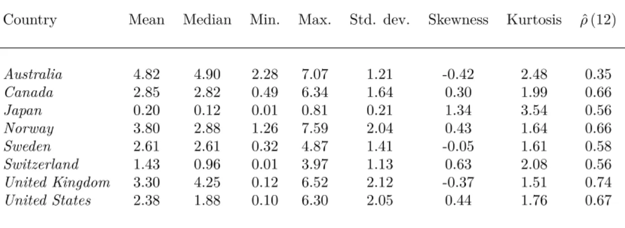
Table 1 shows summary statistics for one-year yields. On average, Australia has the highest one-year yields (4.82%) and Japan has the lowest (0.20%). The well established stylized facts on U.S. yield curves also apply for the rest of the countries in the sample.7 A few features of interest rates during this period
that are worth highlighting are:
1. The yield curves are typically upward sloping. For the most part of the sample, low-maturity yields
are lower than high-maturity yields, except for times of crisis in which the yield curve flattens and even tends to revert - the magnitudes depending on each country’s vulnerability to financial contagion, among other factors. During 2008, for example, Switzerland’s and Norway’s short-term rates not only increased significantly, but the yield curves even inverted, being short-term rates higher than long-term yields for subsequent months.
2. Standard deviation tends to be lower for long-term yields than short-term yields. This is particularly
true during the earlier years in the sample, where short-term yields exhibit high volatility. During the last few years, however, yields have stayed close to the zero lower bound, exhibiting less variability at the short end of the yield curve. Also, some countries exhibit more volatility than others. Japan’s one-year yield, for example, has a standard deviation of 0.21 compared to 2.05 for the U.S. during the same period.
3. Yields are very persistent. The first order autocorrelation is higher than 90% for all countries, with
the most persistent countries being Canada, Norway, the U.K., and the U.S., with an autocorrelation higher than 65% after one year, as seen in table 1. The least persistent country is Australia, with a one-year autocorrelation of 35%.
4. Most yields are close to a normal distribution over the sample period. This is consistent with
contem-porary work that suggests U.S. yields have become more Gaussian in recent years - see for example, Piazzesi (2010). For most countries, skewness is around zero, except for Japan (1.34) and kurtosis ranges from 1.5 (U.K.) to 2.5 (Australia). This suggests that modeling yields under the assumption of a Gaussian distribution is quite reasonable, especially during the time frame considered in the sample.
5. Yields are highly correlated across countries. Table 2 shows the correlation between one-year interest
rates of different countries. Interest rates of the same maturity tend to be very correlated across countries. Although the Japanese yield curve is quite different from other countries’ term structure, particularly during the earlier years, it is most correlated with Australia’s (50%) and Switzerland’s (61%). The U.K., the U.S., and Canada share a correlation above 89%.
6. Yields of near maturity are highly correlated. Table 3 shows the correlation of the 3-month interest
rates of each country with respect to different maturities from 6 months to 10 years. For all countries, the closest the maturity range, the highest the correlation between interest rates of the same country. For example, 3-month and 6-month rates are highly correlated, moving almost one-to-one, but 3-month and 10-year rates tend to differ by country, ranging from 37% (Japan) to 84% (the U.K. and Norway). The exchange rate data are also from Bloomberg L.P, 2014. There are a total of 181 monthly observations per currency from January 1999 to January 2014. All the end-of-month exchange rates are expressed in terms of U.S. dollars (USD) for the following countries: Australia (AUD), Canada (CAD), Japan (JPY), Norway (NOK), Sweden (SEK), Switzerland (CHF), and the United Kingdom (GBP).
Table 4 summarizes the main characteristics of exchange rates during this period. Exchange rates, like interest rates, are very persistent, with an autocorrelation between 57% (GBP) and 79% (CAD) after one year. They are also highly related among themselves, sharing a correlation of 88% or higher, except for the Japanese yen and the British pound, which are the most dissimilar currencies in the sample. The most volatile currencies during this period are the Australian dollar, the Swiss franc, and the British pound with a standard deviation above 0.17, and the least volatile currency is the Japanese yen (0.00). All the currencies exhibit a skewness around zero, from -0.39 (SEK) to 0.83 (JPY), and kurtosis ranges from 1.5 (CAD) to 2.6 (JPY). For the estimation, I calculate annualized log exchange rate changes at different horizons: 1, 3, and 6 months, and 1 to 5 years, in 6-month increments.
3.2
Interest Rate Factors
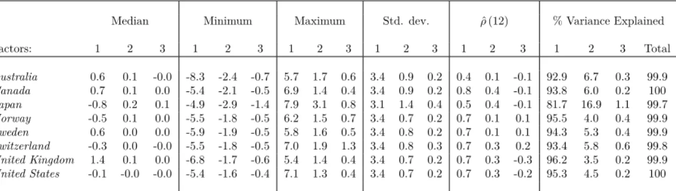
Given the high correlation of yields within each country, the literature has taken advantage of dimensionality-reduction techniques to find the underlying drivers of interest rates. I extract the three main principal components or factors of each country by the eigenvalue-eigenvector decomposition of the variance-covariance matrix of the yields. Typically, the first two or three factors are enough to explain most of the cross-sectional variability in all of the yields. In general, the factors for each country tend to have similar shapes, with Japan’s being the most different. This corresponds to the fact that Japan’s interest rates have been very low for the past decade relative to the rest of the sample.
The first factor is downward sloping, capturing the drop in interest rates that most countries have experienced in the last few years. Table 5 presents summary statistics on the country-specific components. In every country, the first factor extracted from the data is responsible for more than 81% of the cross-sectional variation and the first three factors combined account for more than 99% of total variability. Since the first factor captures most of the variation in all yields within a country, it fluctuates more and has higher standard deviation (around 3.4) than the second (0.8) and third (0.2) factors. Interest rate factors are also very persistent, with the first factor being more persistent than the second and third ones. In term structure models, yields are usually modeled as linear functions of the factors. In this type of setting, that persistence of yields comes from persistent factors, as observed in the data.
Figure 2 shows the loadings or weights that each factor places on the different maturities for every country. The factor loadings exhibit the same pattern: horizontal for the first factor (around 0.3), downward sloping for the second factor, and U-shaped for the third factor. Litterman and Scheinkman (1991) attributed the labels level, slope, and curvature to these three factors given the effect they have on the yield curve. For
example, the first factor affects all yields the same, hence shocks to the first factor generate parallel shifts on the curve, changing the level or average of yields. The second factor loads positively for short-term
maturities and negatively for long-term maturities, thus shocks to the second factor move long and short yields in opposite directions, changing theslope of the yield curve. Finally, the third factor loads positively
on short- and long-term maturities, but negatively on mid-range maturities, thus shocks to the third factor affect thecurvature of the yield curve. The Litterman and Scheinkman (1991) interpretation of the factors
is very common in the literature, although it remains agnostic on links to the macroeconomy.
Recent work provides evidence that the level factor is partly correlated with inflation (Diebold et. al, 2006), aggregate supply shocks from the private sector (Wu, 2006), and shocks to preferences for current consumption and technology (Evans and Marshall, 2007). The slope factor seems to be related to monetary policy shocks (Evans and Marshall, 1998, 2007; Wu 2006) and real activity (Diebold et. al, 2006). However, the curvature factor has not yet been linked to any specific variables. Through my model, the curvature factor helps explain exchange rate fluctuations despite its low contribution to explaining cross-sectional variability in yields. I find some evidence that higher order variables of the yield curve, such as the curvature factor, might be useful in explaining exchange rate movements.
4
Results
The baseline model is estimated by Maximum Likelihood using three observable interest rate factors from each country: level, slope, and curvature. The domestic country is the U.S., therefore exchange rates are
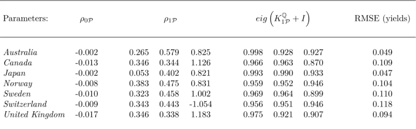
expressed in terms of USD for the 1999-2014 period. First, I present the results for the base line model parameters in annual terms, as well as the term structure fit for each country pair. Next, I evaluate the ability of the model to capture exchange rate movements at different horizons by only using interest rate factors. I explore different model specifications, such as a model with less factors (only the countries’ level and slope) and a model with a different base country instead of the U.S. (the U.K.), as well as several robustness checks. I also explore the implications the model has on the uncovered interest parity puzzle, one of the most relevant puzzles in the exchange rate literature. Finally, I study the implications of my model for ten other countries under a common currency, the euro, and their ability to predict euro-USD fluctuations. Table 6 shows the parameter estimates with asymptotic standard errors in parentheses that correspond to the evolution of the factors under the physical distribution as an unrestricted VAR(1) in equation (6). All parameters are annualized. The first column shows KP
0P ×100. The coefficient of the first factor is always positive, although only sometimes significant, with magnitudes ranging from 0.14 (Canada) to 0.94 (U.S.). The coefficient of the second factor is negative for Australia, Japan, the U.K., and the U.S. and positive for the rest, although not statistically significant. The coefficient of the third factor is statistically significant for all the countries and always positive, except for Switzerland (-0.08). Table 6 also reports estimates of
KP
1P+I. As expected, the diagonal elements are close to one and statistically significant at the 99% level, capturing the fact that interest rate factors are very persistent. The off-diagonal elements of the first and second columns in the VAR are small and insignificant, although the estimates in the third column that correspond to the first factor are larger and negative (around -0.40), ranging from -0.65 (Japan) to -0.14 (Canada), except for Switzerland (0.41), which is positive. Finally, the table reports the lower triangular Cholesky factorization of the variance-covariance matrix, ΣP ×100, which contains large, positive, and significant diagonal elements.
Table 7 reports the parameters of the risk-free rate equation (2), ρ0P and ρ1P, along with the largest eigenvalues of the KQ
1P +I matrix, and a measure of goodness of fit of model-implied yields. ρ0P is always negative between -0.017 and -0.002,ρ1P is always positive, and each factor’s estimate ofρ1P increases, being the third factor estimates close to one for all countries, except for Switzerland (-1.054). The eigenvalues of the transition matrix under risk-neutrality are large and close to one, hence shocks to these factors have permanent effects in their evolution over time. As a measure of goodness of fit, the last column reports root mean square errors (RMSE) in basis points for the cross-section of yields. The RMSE is around 10 basis points, with the best fit for the Japanese yen (4.7) and Australian dollar (4.9) and the worst fit for the Swiss franc (11.8). Overall, the goodness of fit for interest rates is very good, as it is standard in term structure models of interest rates, which suggests that the incorporation of exchange rates into the model does not compromise the fit of the yield curve.
4.1
Exchange Rate Fit
In order to obtain a general measure of goodness of fit for exchange rates, I project the exchange rate data on the model-implied exchange rates. Hence, given the model equation describing annualized log exchange rate changes at differentk horizons,
∆st+k =rtd+k−1−r f t+k−1+ 1 2 h Λdt+0k−1Λdt+k−1−Λ f0 t+k−1Λ f t+k−1 i + Λdt+0k−1dt+i−Λ f0 t+k−1 f t+i, (22)
I perform an ordinary least squares (OLS) regression of the data on the model-implied exchange rate equations for each currencyi,
∆sobs,it+k =αi+βi∆sit+k+µit+k. (23)
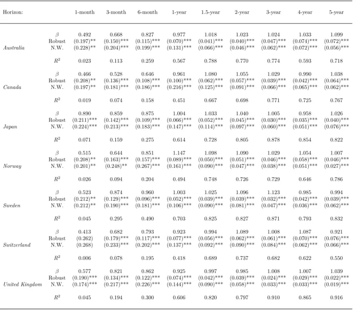
Table 8 displays the results from regression (23), which account for the goodness of fit of the annualized model-implied exchange rate changes at differentkhorizons, from 1 month to 5 years. This model determines the exchange rate changes as a function of six total factors (the level, slope, and curvature of each country). The domestic country is chosen to be the U.S. so that the exchange rates are in terms of USD prices. Therefore, an increase in ∆strepresents a depreciation of the U.S. dollar with respect to the foreign currency,
i. The results for βi, along with the corresponding standard errors and the adjusted R2, are reported for
selected horizons: 1 , 3 , and 6 months, and 1 , 1.5 , 2 , 3 , 4 , and 5 years.
At the one-month horizon, the fit of the model, as measured by theR2, ranges from 1% and insignificant
(Switzerland) to 7% and statistically significant at the 99% confidence level (Japan). Very short exchange rate fluctuations are quite difficult to predict. Meese and Rogoff (1983) claimed that the best forecasting model is obtained under the assumption that the exchange rate follows a random walk. However, at longer horizons the predictability of exchange rates improves significantly. This type of behavior is observed in other assets as well. Although short-term movements are not well understood, it seems that at longer horizons the factors are better able to capture the signal that drives movements in asset returns. Figure 3 shows the annualized one-month log changes in exchange rates for all the currencies relative to the USD as well as the model-implied expected exchange rate fluctuations. Overall, the expected exchange rate changes implied by the model are not as volatile; however, they capture the data movements on average quite well.
In general, the regression coefficients increase in magnitude and significance as the horizons increase. At the one-year horizon and thereafter, the coefficients of all currencies are close to one. Approximately half of the variation in one-year exchange rate movements can be explained by the model using interest rate factors
alone, for all currencies relative to the USD. Figure 4 shows the data and model-implied one-year expected fluctuations in the exchange rate. The fit of the model at this horizon ranges from 41.8% for the Swiss franc to 70.3% for the Swedish krona. The model is even more successful at capturing five-year exchange rate movements, depicted in figure 5, ranging from 55% (Swiss franc) to 91.6% (British pound).
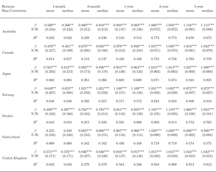
One of the potential concerns within this framework is small-sample bias. Because the closer to a unit root, the larger the small-sample bias in Maximum Likelihood estimates, Joslin, Singleton, and Zhu (2011) enforce a high degree of persistence under the physical distribution of the factors to ensure a stationary process, by which they constrain all the eigenvalues that govern the speed of mean reversion to be strictly positive. Small-sample bias arises due to the high persistence of the factors, and becomes particularly problematic when the sample period is short. To this end, I estimate robust (White) standard errors and Newey-West standard errors to account for small-sample bias and for potential correlation and heteroskedasticity in the innovation vector. This generates larger standard errors that specify the precision of the estimated coefficients. Similar to Lustig, Roussanov, and Verdelhan (2011), I follow Andrews (1991) to choose the number of lags for the Newey-West estimation to be the horizonk(in months) plus one. After the three-month horizon, all of the estimates are statistically significant at the 99% confidence level regardless of the method used to calculate standard errors, except for the Norwegian krone under Newey-West standard errors that is significant at the 95% level.
Bauer, Rudebusch, and Wu (2012, 2014) argue that this method still leads to large biased estimates that may yield an inconsistent risk premium. Given the separation argument, only the parameters that characterize the physical density of yields are affected. They propose to replace the initial estimates of the factors’ vector auto-regressive process underPwith simulation-based bias-corrected estimates and then
proceed to the Maximum Likelihood estimation. I therefore implement their suggested inverse bootstrap bias-corrected method: For each of the 5,000 bootstrap iterations (after discarding the first 1,000), I simulate a set of 50 bootstrap samples using some trial parameters and calculate the mean or median of the OLS estimator to be equal to the original OLS estimate. The bias-corrected estimates then reflect more persistent factor dynamics, as measured by the largest eigenvalues of the transition matrix. More details on the estimation of bias-corrected factor dynamics and the consequences of OLS bias in term structure models can be found in Bauer, Rudebusch, and Wu (2012, 2014).
Table 9 shows the exchange rate fit for the model after adjusting for mean and median bias-corrected estimates for selected maturities with the coefficients from regression (23), Newey-West standard errors in parenthesis, and R2 adjusted for degrees of freedom. As expected, the VAR physical dynamics are more
persistent after correcting for bias, either by mean or median correction, although estimates for ΣP remain close to the estimates of the unrestricted VAR. After estimates are corrected for bias (either by the mean
or the median) interest rate factors are still able to explain as much variation in exchange rates. The same patterns as the base model can be observed: at the one-month horizon, the best fit is the Japanese yen (6%) and the worst is the Swiss franc (0%), and as the horizon increases, the fit of the model improves for all currencies. Exchange rate changes at the one-year horizon and thereafter have coefficients around one that are statistically significant at the 99% confidence level, and about 50% of one-year exchange rate movements can be explained by the model, from 43% (Swiss franc and Canadian dollar) to 60% (Japanese yen and Swedish krona). For some currencies, correcting for bias reduces the fit of the exchange rate model, but for some currencies (Norwegian krone and Swiss franc), it improves it. Most importantly, the results are still quite similar, and at the five-year horizon, the model accounts for 57% to 91% of exchange rate movements using interest rate factors alone.
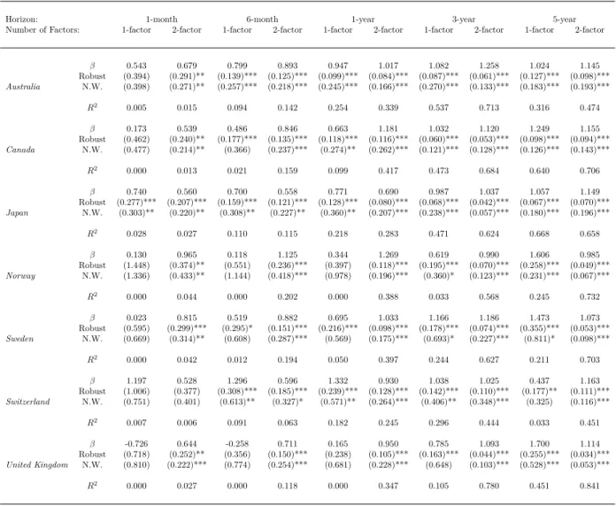
I next evaluate the performance of the model with a different number of factors. Table 10 reports the estimates for selected maturities of a linear projection of the data on a model with only one factor, the level, or two factors, the level and the slope, for each country. With fewer interest rate factors, the root mean square errors that measure the term structure fit of each country increase relative to the three-factor model. The two-factor model has RMSEs that are from 1.4 basis points (Switzerland) to 17.1 basis points (Canada) higher than the three-factor model. In contrast to the base model, the two-factor model exhibits coefficients ofρ0P that are positive for all countries, except for Sweden, and the coefficients of ρ1P are positive, except for Japan’s first factor, with the second coefficient being larger than the first. The physical distribution parameters do not exhibit significant differences in signs or magnitudes. The one-factor model exhibits larger RMSEs than the other models, as expected, ranging from 43.4 basis points for Norway to 103.9 for Canada.
In general, the same pattern emerges for all models: the exchange rate fit improves at longer horizons. In every case, the two-factor model outperforms the one-factor model, although they are both well below the performing levels of the three-factor model. That is, adding a third factor to the model, the curvature factor, significantly improves the model’s ability to explain exchange rates, despite having low-content information to explain cross-sectional interest rate variation.
A few highlights of these lower-factor models are worth mentioning. For Norway, Sweden, and the U.K., the one-factor model can explain less than 5% of exchange rate movements at horizons one-year or lower, so for these countries most of the valuable information in explaining short-term exchange rate fluctuations actually comes from the other components, the slope and curvature. However, the one-factor model does remarkably well for Australia and Japan, over 20% of one-year changes are captured by the countries’ level alone, which suggests that Japan’s and Australia’s level factor may contain a lot of information about their exchange rate movements. Finally, the two-factor model explains exchange rate changes extremely well for
Canada relative to the three-factor model, which suggests that incorporating the curvature factor does not seem to significantly contribute to modeling the CAD-USD exchange rate path. Given the relevance of the curvature factor in modeling most currency movements in the long run, the third yield curve component could be capturing long run expectations on exchange rate fluctuations or other fundamentals relative to international markets that influence the exchange rate.
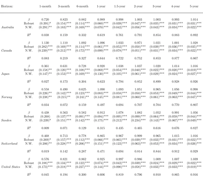
I also re-estimate the model considering a different base country, the U.K., so that exchange rates are in terms of the British pound, instead of the U.S. dollar. Table 11 reports the coefficients, robust and Newey-West standard errors, and the adjustedR2 for all countries in which the log exchange rate changes
are modeled in terms of the British pound. The model parameters are very similar, for example, ρ0P and
ρ1P have the same sign and similar magnitude regardless of the base country, includingρ13P for Switzerland, which is negative one as well. Notice that modeling the USD-GBP exchange rate is the same as modeling the GBP-USD exchange rate, since results are symmetric. This is because it does not matter what country is selected as domestic and what country is selected as foreign; the information content in the factors is still the same. Hence the regression results for the U.S. dollar in terms of the British pound from table 11 are the same as the results for the British pound in terms of the U.S. dollar from table 8.
For the other countries results are similar, although not the same, since instead of the U.S. term structure we are now modeling exchange rates with U.K. interest rate factors, which exhibit different shapes. In general, results are similar whether one is using the U.S. or the U.K. as a base: The coefficients are significant at the 99% confidence level after 3 months (except for Norway under N.W. standard errors, which is significant at a 95% confidence level, just as in the base model).
For exchange rate fluctuations in the Australian dollar, Canadian dollar, Japanese yen, and Swiss franc, results are either slightly better or significantly better when using the U.K. as a country base. For example, the Swiss franc, which has the worst fit at most maturities when modeled with respect to the U.S. dollar, significantly improves the fit with a 47% R2 at the one-year horizon and 92% at the five-year horizon, in
contrast with 41% and 55% under the USD, respectively. In the base model, 45% of one-year CAD-USD exchange rate fluctuations are explained by the factors, whereas the model with U.K. factors accounts for more than 64% of the CAD-GBP one-year exchange rate. Moreover, except for Sweden, all other currencies experience a better fit at the five-year horizon when modeled in terms of the British pound, withR2 from 80% (NOK) to 92% (JPY and CHF). Estimates for the Nordic countries explain less of the exchange rate movements when the GBP is used as a base. For Norway, results are slightly worse, whereas for Sweden, a lot worse. This may suggest that some countries have more information than others about expected exchange rate movements, although we can say with certainty that the U.S. is not particularly more informative than other countries, such as the U.K.
4.2
Implications in the context of the UIP Puzzle
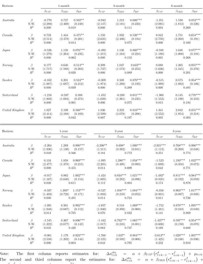
In this section, I evaluate my model in the context of the Uncovered Interest Parity (UIP) puzzle. UIP claims that any excess return on foreign-denominated deposits is offset by the expected depreciation against the domestic currency. That is, if we run the following regression
∆sobst+k=α+βU IP rdt+k−1−r f t+k−1 +µt+k (24)
we would expect that α = 0, βU IP = 1.8 However, the data do not hold against this proposition, since the coefficient of the interest rate differential is not only different from one, but also negative, and the explanatory power of the interest rate differential is very low. Several papers have focused on studying this phenomenon.9 In my model, the UIP condition does not hold, since the expected log exchange rate change
is not only a function of the interest rate differential but also a function of a risk premium term implied by my framework: ∆sobst+k =α+βIRD rtd+k−1−rtf+k−1+βRP 1 2 h Λdt+0k−1Λdt+k−1−Λft+0k−1Λft+k−1i +µt+k. (25)
This is consistent with the idea proposed by Fama (1984) and Hansen and Hodrick (1983), that attribute the anomalous findings to a time-varying risk premium. I evaluate the ability of my model to reproduce the UIP puzzle when equation (24) is estimated and I examine to what extent, the augmented UIP regression implied by my model, equation (25), can help solve the puzzle.
Table 12 shows the results for the UIP and augmented-UIP regressions. The coefficient of the UIP regression, βU IP, is sometimes positive, sometimes negative, but never statistically significant in the short run. At longer horizons (after two years), some coefficients are significant but always large and negative. Moreover, the adjusted R2 is below 5% for one-year or lower frequency changes for every country. This is
consistent with the UIP puzzle observed in the data.
When incorporating the model-implied risk premium, the adjusted R2 always increases, the coefficient of the interest rate differential,βIRD is always positive (except for Switzerland at the one-month and three-month horizon) although only statistically significant at longer horizons. For the three-year horizon, the interest rate differential is close to one for every currency and the coefficients are statistically significant at
8Notice that this regression is a slight variation from the standard UIP regression, since the interest rate differential is
lagged one period with respect to the log exchange rate changes. This is because the interest rate differential component comes from the model and it is constructed as a linear function of the factors. Standard UIP regressions use the actual interest rate differential from the data with yields of the corresponding maturityk, such as, for example, Flood and Taylor (1996) or Dong (2006). The idea in this case is to evaluate the interest rate differential implied by the model.
the 99% confidence level, with the lowest coefficient being 0.60 for the Swiss franc. The coefficient of the risk premium,βRP, is always positive, approaches one, and becomes statistically significant at the 99% confidence level for every country after the three-month horizon (except for Norway, which is statistically significant at the 95% level). These results suggest that the risk premium term is clearly important in modeling exchange rates, even when only interest rate factors are considered, and contributes to closing the gap with respect to the UIP puzzle.
Besides attributing the failure of UIP to the presence of a time-varying risk premium, Fama (1984) identified two conditions necessary for the risk premium to solve the UIP puzzle. First, the risk premium has to be more volatile than the interest rate differential, and second, the model-implied risk premium and the interest rate differential need to be negatively correlated. Table 13 shows that the Fama conditions hold for all currencies and for all horizons considered. The variance of the risk premium is higher than the variance of the interest rate differential by a magnitude of two or higher. Also, the correlation between the interest rate differential and the risk premium is always negative and large as it increases in horizon, as expected. This suggests that the risk premium implied by the model with interest rate factors is a key driver of exchange rates, which is consistent with Fama (1984) and Hansen and Hodrick (1983) explanation of the UIP puzzle, and does not rely solely on large shocks to drive movements in the exchange rate.
4.3
Implications for the Euro Dynamics
In the baseline model, the factors extracted from two countries help determine their exchange rate fluctua-tions through each countries’s stochastic discount factor. However, when multiple countries share the same currency, what are the factors that determine movements in, for example, the euro-U.S. dollar exchange rate?
I explore the determination of the path of the euro by estimating the stochastic discount factor of ten countries under the euro regime: Austria, Belgium, Finland, France, Germany, Ireland, Italy, the Nether-lands, Portugal, and Spain. That is, I estimate pricing kernels for those countries individually to explore whether their interest rate factors alone contribute to explaining changes in the euro (EUR). My model allows one to observe whether any particular country in the Euro area has more useful information on the EUR-USD exchange rate fluctuations than others.
Figure 6 shows the evolution of yield curves for each country. Although some term structures exhibit similarities, such as Germany’s, Finland’s, and the Netherlands’, other countries behave quite differently, such as Ireland, Portugal, Italy, or Spain; these countries exhibit different yield curve movements, particularly during the 2011-2012 European crisis. Although the short rate increased for every European country during
that time, some were more susceptible to the Greek crisis than others, with their short rates reaching significantly higher levels. For example, Portugal’s interest rates rose to 17% in January 2012. Because these countries exhibit different yield curves, interest rate factors extracted from each term structure will also be quite different.
Which country can explain euro fluctuations the most? As expected, the yield curve factors for a country such as Germany are important in determining changes in the euro. However, risk factors from countries with more volatile interest rates, such as Italy and Spain, also have high explanatory power on the exchange rate dynamics. For example, Italy has higher explanatory power over euro-USD fluctuations than Germany at every horizon. The results suggest that the risk factors that govern fluctuations in the euro are priced to a similar extent in the yield curves of different European countries.
Table 14 reports the results of the linear projection of euro movements on the model-implied exchange rates for ten European countries in terms of the U.S. dollar. All countries seem to have similar degrees of explanatory power on the euro. In general, the same conclusion holds for this set of countries: exchange rate fit improves at longer horizons and the addition of a curvature factor generally improves the fit of the model. At the one-year exchange rate horizon, all the countries are able to explain around 50% of exchange rate movements. Ireland and Finland exhibit the worst fit (39% and 40%), while Italy, Spain, Portugal, and Belgium show the best fit (58%, 51%, 50%, and 50%). However, at the five-year horizon, every country is able to explain 83% or more of the total variation in the EUR-USD exchange rate, with the lowest being Austria (83.8%) and Spain (88.6%) the highest. After the three-month horizon, every country is statistically significant at the 99% confidence level, except for Finland and Portugal, which are significant at the 95% level with N.W. standard errors. Results are quite similar regardless of what country is the base, the GBP or the USD. These results suggest that currency risk in the euro is priced in every European country, and term structure cross-sectional variation captures those expectations really well.
5
Conclusion
This paper examines whether interest rate factors alone can help determine fluctuations in the exchange rate using a no-arbitrage term structure model. I propose a framework that models exchange rate changes at different horizons as the ratio of two countries’ stochastic discount factors in which most of the variation is driven by a nonlinear risk premium. The results suggest that interest rate factors are indeed helpful in modeling exchange rates, particularly at longer horizons. These results are in line with findings by Mark (1995), who identifies a predictable component in exchange rate fluctuations as the horizon increases. Key to my results is the fact that interest rate factors extracted from the yield curve are observable, which allows
for a straight forward estimation of the model by Maximum Likelihood as in Joslin, Singleton, and Zhu (2011).
Interest rate factors, level, slope, and curvature, can explain half of the variation in one-year exchange rates for countries with free-floating currencies from 1999 to 2014: Australia, Canada, Japan, Norway, Sweden, Switzerland, and the U.K., with respect to the U.S. dollar. Moreover, the fit of the model improves as the horizon increases, suggesting that long-term expected fluctuations in the exchange rate are captured by yield curve factors. Results are robust to accounting for small-sample bias, potential heteroskedasticity in the error term, and across multiple currencies relative to a different base. A drawback in the literature is that there is no clear link between interest rate factors and the macroeconomy, particularly the curvature factor. In this paper, I present evidence that despite of the curvature factor explaining a small fraction of yield curve movements, it provides a significant contribution to explaining exchange rates. When using fewer factors, either the level or the level and slope, the explanatory power of the model decreases, suggesting that the curvature factor is important in explaining exchange rate fluctuations for most currencies in the sample. A key implication of the model is that a risk premium, nonlinear in the interest rate factors, drives most of the variation in exchange rates. Further analysis in the context of the uncovered interest parity puzzle suggests that the model-implied risk premium satisfies the Fama (1984) conditions: is negatively correlated with the interest rate differential and exhibits significantly larger variance. This two-country term structure model with observable interest rate factors is quite successful at deriving stochastic discount factors that imply a theory-consistent risk premium. Moreover, this paper explores the ability of ten European countries to account for fluctuations in the euro by only using their own interest rate factors. Although European countries exhibit different yield curves, they all capture exchange rate movements to a similar extent, suggesting that exchange rate risk is implicit in yield curves of every European country in the sample. Further work on this area includes exploring whether these results are time-independent, or if during crises, certain European countries capture exchange rate information better than others.
There remain multiple avenues to be explored within this framework. Given that this work presents evidence of interest rate factors’ explanatory power over exchange rate movements at different horizons, a possible extension is to investigate the factors’ ability to forecast exchange rates out of sample. Despite the large body of literature devoted to modeling exchange rates, there is a high degree of uncertainty about how exchange rates react to changes in expectations, particularly out of sample.
Motivated by the idea that a unique stochastic discount factor should be able to account for prices of different assets, another extension of this paper is to incorporate equities. Given that the same stochastic discount factor prices securities in the bond and foreign exchange markets, it should price securities in the equity market as well. Similarly to exchange rates, the equity returns literature also finds a long-run