RAID for Enterprise Computing

(1)

A T E C H N O L O G Y W H I T E P A P E R from VERITAS Software Corporation

fpA RAID technology and implementation

backgrounder to help system administrators

and application designers make intelligent

on-line storage subsystem choices.

(2)

(3)

Figures

FIGURE 1: HOST BASED AND CONTROLLER BASED DISK ARRAYS... 5

FIGURE 2: MIRRORING: THE SIMPLEST FORM OF RAID ... 10

FIGURE 3: PARITY RAID ... 11

FIGURE 4: SOME POPULAR PARITY RAID ARRAY SIZES... 12

FIGURE 5: EXCLUSIVE OR PARITY IN A THREE DISK ARRAY... 14

FIGURE 6: USING EXCLUSIVE OR PARITY TO REGENERATE USER DATA... 15

FIGURE 7: EXCLUSIVE OR PARITY IN A FOUR DISK ARRAY... 16

FIGURE 8: DATA STRIPING... 18

FIGURE 9: LOCATING DATA BLOCKS IN A STRIPED ARRAY... 19

FIGURE 10: HOST-BASED STRIPING OF CONTROLLER-BASED PARITY RAID ARRAYS... 20

FIGURE 11: EFFECT OF DATA STRIPING ON FILE LOCATION... 22

FIGURE 12: EFFECT OF DATA STRIPING ON I/O REQUEST DISTRIBUTION... 23

FIGURE 13: DATA STRIPING FOR DATA TRANSFER INTENSIVE APPLICATIONS... 24

FIGURE 14: RELATIVE PERFORMANCE OF STRIPED ARRAYS... 25

FIGURE 15: GATHER WRITING AND SCATTER READING... 27

FIGURE 16: DATA STRIPING WITH PARITY RAID ... 28

FIGURE 17: ONE WRITE ALGORITHM FOR A PARITY RAID ARRAY... 29

FIGURE 18: OPTIMIZED WRITE ALGORITHM FOR A PARITY RAID ARRAY... 31

FIGURE 19: RAID ARRAY WITH DATA STRIPING AND INTERLEAVED PARITY... 32

FIGURE 20: RELATIVE PERFORMANCE OF PARITY RAID ARRAYS... 33

FIGURE 21: DATA STRIPING COMBINED WITH DATA MIRRORING... 34

FIGURE 22: USING BREAKAWAY MIRRORED DATA FOR BACKUP WHILE THE APPLICATION EXECUTES... 36

FIGURE 23: MIRRORING AND FAILURE RATES... 41

FIGURE 24: PARITY RAID AND FAILURE RATES... 42

Tables

TABLE 1: SUMMARY COMPARISON OF COMMON FORMS OF RAID ... 8

(4)

(5)

RAID for Enterprise Computing

RAID has become commonplace in server computing environments. Today, most disk subsystems incorporate RAID technology to enhance their I/O performance and data availability. Software, or host-based RAID is also available from several ven-dors, including VERITAS. System administrators, application designers, and others responsible for implementing their organizations’ storage strategies are faced with a number of choices. This paper outlines the basics of RAID technology, describes the advantages of the various RAID alternatives, and lists other considerations in devel-oping technical strategies for enterprise storage.

What’s in a Name?

RAID is an acronym for Redundant Array of Independent Disks:

➨ Redundant means that part of the disks’ storage capacity is used to store check

data that can be used to recover user data if a disk containing it should fail.

➨ Array means that a collection of disks are managed by control software that

presents their capacity to applications as a set of coordinated virtual disks. In

host based arrays, the control software runs in a host computer. In controller based arrays, the control software runs in a disk controller.

➨ Independent means that the disks are perfectly normal disks that could function

independently of each other.

➨ Disks means that the storage devices comprising the array are on-line storage.

In particular, unlike most tapes, disk write operations specify precisely which blocks are to be written, so that a write operation can be repeated if it fails.

RAID Controller Host Computer Host Computer

Host Based Array Controller Based Array

9 9 9 9

(6)

The World’s Shortest History of RAID

The Berkeley “RAID Levels”

In the late 1980s, researchers at the University of California at Berkeley were looking for ways of combining disks into arrays with desirable combinations of affordability, data availability and I/O performance. In 1988, a landmark paper entitled A Case for

Redundant Arrays of Inexpensive Disks was published. The paper demonstrated that

arrays of low-cost personal computer disks could be effective substitutes for the high

capacity, high performance disks then used with data center computers. Five disk ar-ray models, called RAID Levels, were described. The paper described each RAID level in terms of:

➨ a mechanism for using redundant check data stored on separate disks to recover user data lost due to disk failure, and,

➨ an algorithm for mapping user data and check data blocks onto physical storage resources for optimal I/O performance.

The first RAID Level described in A Case for Redundant Arrays of Inexpensive

Disks was mirroring, already in commercial use at the time. The remaining four

RAID Levels were essentially proposals to industry to build more cost-effective, more generally applicable types of arrays. Some of the RAID Levels, notably Levels 2 and 3, required special purpose disk or controller hardware. Although examples of both were built, special purpose hardware produced in low volume made them eco-nomically unattractive, and neither is commercially available today.

RAID Today

Of the five RAID Levels described in A Case for Redundant Arrays of Inexpensive

Disks, two are of commercial significance today:

➨ RAID Level 1, or disk mirroring. RAID Level 1 provides high data reliability at

the cost of an “extra” check data disk (and the host bus adapter port, housing, cabling, power, and cooling to support it) for every user data disk. Most mirror-ing implementations deliver somewhat better read performance than an equiva-lent single disk, and only slightly lower write performance.

➨ RAID Level 5, called parity RAID later in this paper, interleaves check data (in

the form of bit-by-bit parity) with user data throughout the array. A RAID Level 5 array’s disks may operate independently of each other, allowing multi-ple small application I/O requests to be executed simultaneously, or they may

(7)

operate in concert, providing parallel execution of large application I/O re-quests.

RAID Level 5 is ideally suited for any applications whose I/O consists princi-pally of read requests. Many transaction processing, file and database serving, and data analysis applications fall into this category. Particularly in host-based implementations, Raid Level 5 is not well suited for write-intensive applications such as data entry or scientific and engineering data collection.

Other Forms of RAID

In 1989, the authors of A Case for Redundant Arrays of Inexpensive Disks published another paper entitled Disk System Architectures for High Performance Computing, in which a sixth RAID model offering protection against two concurrent disk failures was described. This model became known as RAID Level 6. For large arrays, RAID Level 6 provides extremely high data availability (much higher than mirroring) at modest incremental storage cost. It is complex to implement, however, and has a larger inherent write penalty than RAID Level 5.

The acronym RAID is commonly used to describe two other types of disk array:

➨ RAID Level 0: This term is commonly used to describe arrays in which data is

striped across several disks (as described later in this paper), but without any

check data. Striped arrays provide excellent I/O performance in a wide variety of circumstances, but offer no protection against data loss due to disk failure.

➨ RAID Level 0+1: Also known as RAID Level 1+0 in a slightly different form,

this type of array consists of pairs of disks across which data is striped. Al-though multi-disk mirrored arrays were described under the heading RAID Level 1 in A Case for Redundant Arrays of Inexpensive Disks, the industry and market have adopted the RAID Level 0+1 nomenclature to describe this type of array.

Table 1 (page 8) compares the cost, data availability, and I/O performance of the commonly known RAID Levels. In Table 1, I/O performance is shown both in terms of large I/O requests, or relative ability to move data, and random I/O request rate, or relative ability to satisfy I/O requests, since each RAID Level has inherently different performance characteristics relative to these two metrics. Each RAID Level’s par-ticular strong points are highlighted in the table by shading.

(8)

RAID Type Common Name Description Relative Cost (Disks) Relative Data Availability Large Read Data Transfer Speed1 Large Write Data Transfer Speed Random Read Request Rate Random Write Request Rate

0 Data Striping User data distributed across the disks in the array.

No check data.

N lower than single-disk

very high very high very high very high

1 Mirroring User data duplicated on N separate disks. (N is usually 2).

Check data is second copy (as in Figure 20)

N higher than

RAID Level 3, 4, 5; lower than RAID

Level 2, 6

higher than single disk (up to 2x)

Slightly lower than single disk

up to Nx single disk similar to single disk

“0+1” Striped Mirrors User data striped across M separate pairs of mirrored disks.

Check data is second copy (as in Figure 2)

2M higher than

RAID Level 3, 4, 5; lower than RAID

Level 2, 6

much higher than single disk

higher than single disk

much higher than single disk

higher than single disk

2 User data striped across N disks Hamming code check data distributed across m disks, (m is determined by N).

N+m higher than RAID Level 3, 4, 5

highest of all listed types

approximately 2x single disk

3 RAID 3,

Parallel Transfer Disks with Parity

Synchronized disks

Each user data block distributed across all data disks.

Parity check data stored on one disk.

N+1 much higher than single disk; comparable to RAID

2, 4, 5

highest of all listed types

approximately 2x single disk

4 Independent disks

User data distributed as with striping. Parity check data stored on one disk. (as in Figure 16)

2, 3, 5

similar to disk striping

slightly lower than disk striping

similar to disk striping

significantly lower than single disk

5 RAID 5,

“RAID”

Independent disks

User data distributed as with striping; Parity check data distributed across disks. (as in Figure 19)

2, 3, 4

slightly higher than disk striping

slightly lower than disk striping

Slightly higher than disk striping

Significantly lower than single disk;

higher than RAID Level 4 6 RAID 6 As RAID Level 5, but with additional

inde-pendently computed distributed check data.

N+2 highest of all listed types

slightly higher than RAID Level 5

lower than RAID Level 5

slightly higher than RAID Level 5

lower than RAID Level 5

Table 1: Summary Comparison of Common Forms of RAID

(9)

Inexpensive or Independent?

A Case for Redundant Arrays of Inexpensive Disks generated considerable interest

among users because it referred to Inexpensive Disks. The paper argued that RAID could substantially lower storage costs in large computer systems through the use of inexpensive disks.

Had disk technology remained static for the last ten years, this would still be the case. While RAID was gaining acceptance, however, disk costs were dropping rapidly. To-day, the low cost personal computer disk and the data center disk are nearly the same device. The disks used in RAID arrays are no longer inexpensive relative to data center disks. The inherent cost of RAID must therefore be compared to that of equivalent usable disk capacity without RAID capability.

Today, RAID arrays no longer provide inherently inexpensive storage. RAID tech-nology, however, has significantly “raised the bar” for data availability and I/O per-formance, so RAID is highly valued by storage buyers. By common consent, there-fore, the industry and market have transmuted the RAID acronym to stand for Redun-dant Arrays of Independent Disks.

What Ever Happened to RAID 3?

As described in A Case for Redundant Arrays of Inexpensive Disks, the disks of a RAID Level 3 array would rotate synchronously, with each block of user data subdi-vided across all but one of them (the remaining disk would contain parity). Strict in-terpretation of this proposal would have required highly specialized disks, buses, and controllers. Since these would have been prohibitively expensive, RAID Level 3 sub-systems were typically approximations implemented with conventional disks.

As Table 1 asserts, RAID Level 3 performs well with large sequential I/O requests. This is because data transfer is divided among all but one of an array’s disks, which operate in parallel to get it done faster. As this paper will demonstrate, however, RAID Level 4 and RAID Level 5 can deliver nearly equal performance for large se-quential I/O requests. Moreover, since the first RAID products were introduced, cache has become ubiquitous in RAID subsystems (and in host based implementa-tions as well), masking individual disk interacimplementa-tions to some extent.

The result of these factors has been a diminished motivation for specialized RAID Level 3 arrays, which are only good at large sequential I/O loads, in favor of more generally applicable RAID Level 5 products. A few vendors still offer RAID Level 3 capability (which tends to be implemented by manipulating data layout), but most simply offer a more generally applicable RAID Level 5, or parity RAID.

(10)

RAID Technology Basics

The Two Fundamental RAID Concepts

Virtually all RAID implementations incorporate two concepts:

➨ data redundancy, in the form of check data, which enhances user data

avail-ability by enabling the recovery of user data if the disk containing it should fail.

➨ data striping, which enhances I/O performance by balancing I/O load across

the disks comprising an array.

Both concepts are implemented by the array’s control software. The concepts are in-dependent. Either can be (and indeed, occasionally is) implemented without the other. Most often, however, disk array subsystems incorporate both concepts and therefore deliver both high data availability and excellent I/O performance.

Data Redundancy

The redundancy in RAID refers to the use of part of the disks’ capacity to store more than one copy of user data. In its simplest form, mirroring, redundancy is easy to un-derstand—a second copy of data stored on a second disk leaves user data accessible if either of the disks fails. Figure 2 illustrates this.

Disk Block 000 User Data Block 000

• • •

Disk A Disk Block 002 Disk B

User Data Block 002 Disk Block 001

User Data Block 001

Each block written by an application must be written to both disks Any block read by an application may

be read from either disk

etc. etc.

Figure 2: Mirroring: The Simplest form of RAID

Figure 2 illustrates RAID Level 1, often called mirroring because the data stored on each disk is a mirror image of that stored on the other. In a mirrored array, the control

(11)

software executes each application write request twice—once to each disk. Each

block on a disk is the check data for the corresponding block of user data on the other disk. When an application makes a read request, the control software chooses one of the disks to execute it. Some control software implementations improve performance by choosing the least busy disk to satisfy each application read request.

Mirrored data remains available to applications if one of the mirrored disks fails. It has the drawback of being relatively expensive. For every disk of data, the user must purchase, house, power, cool, and connect two disks.

Parity RAID Redundancy

RAID Levels 3, 4, and 5 all rely on another type of redundancy called parity. Parity RAID reduces the cost of protection (requires fewer “extra” disks), but protects against fewer failure modes. Instead of a complete copy of every block of user data, each block of parity RAID check data is computed as a function of the contents of a

group of blocks of user data. The function allows the contents of any block in the

group to be computed (“regenerated”), given the contents of the rest of the blocks. Figure 3 illustrates the principle of parity RAID.

• • •

Disk A Disk B

Disk Block 002

on Disk B User Data Block 001

on Disk B Each time a block is written, the corresponding

check data block must be recomputed and rewritten Multiple application read requests can be satisfied

simultaneously as long as they specify data on different disks

Check Data Block 000

• • • Disk C

User Data Block 000 on Disk A

etc. etc.

etc.

User Data Block 000

User Data Block 001

User Data Block 002

User Data Block 000

User Data Block 001

User Data Block 002

Figure 3: Parity RAID

In Figure 3, Disk A and Disk B hold user data. Each block of Disk C holds check data computed from the corresponding blocks from disks A and B.

➨ If Disk A fails, any block of data from it can be regenerated by performing a computation that uses the corresponding blocks from Disks B and C.

➨ If Disk B fails, any block of data from it can be regenerated by performing a computation that uses the corresponding blocks from Disks A and C.

(12)

➨ If Disk C fails, only protection is lost, not user data.

The “Cost” of Parity RAID

The overhead cost of data protection in the parity RAID array illustrated in Figure 3 is lower than that of the mirrored array of Figure 2—one “extra” disk for every two disks of user data, compared to an extra disk for each disk of user data with mirroring. Parity check data is computed as a bit-by-bit exclusive OR of the contents of all cor-responding user data disk blocks. Using parity as check data allows the construction of arrays with any number of data disks using only one parity disk. Thus, while the array illustrated in Figure 3 has an overhead “cost” of 50% (1.5 physical disks are re-quired for each disk of user data storage), larger parity RAID arrays with much lower overhead cost are possible. For example, an eleven disk parity RAID array could hold ten disks of user data, for an overhead cost of 10%. Figure 4 illustrates some of the more popular parity RAID array size encountered in practice.

“Three plus one” array overhead cost: 33%

“Four plus one” array overhead cost: 25%

9 9 9

9 9 9 9 9

9 9 9 9 9 9 9 9 9 9 9

9

9 9 9 9 9

“Five plus one” array overhead cost: 20%

“Ten plus one” array overhead cost: 10%

9

Data Disk

Check Data

Figure 4: Some Popular Parity RAID Array Sizes

If a single check data disk can protect an arbitrarily large number of user data disks, the strategy for designing parity RAID arrays would seem to be simple: designate one check data disk and add user data disks as more storage capacity is required. There are disadvantages to parity RAID large arrays, however.

Disadvantages of Large Parity RAID Arrays

(13)

➨ Parity check data protects all the disks in an array from the failure of any one of them. If a second disk in a parity RAID array fails, data loss occurs.2_{A three}

disk parity RAID array “fails” (results in data loss) if two disks out of three fail simultaneously. A six disk parity RAID array fails if two disks out of six fail simultaneously. The more disks in an array, the more likely it is that two disk failures will overlap in time and cause the array itself to fail. Moreover, when an array fails, all the data stored in it usually becomes inaccessible, not just data from the failed disks. Thus, the larger the array, the more serious the conse-quences of failure are likely to be. Smaller arrays reduce the probability of array failure, and mitigate the consequences if one does occur.

➨ Large parity RAID arrays have poor write performance. Later in this paper, writing data to a parity RAID array will be described. For now, it is sufficient to note that when an application writes a single block of data to a parity RAID ar-ray, computations must be performed, and blocks must be both read and written on two of the array’s disks. In addition, the control software must keep some type of persistent3_{log in case of a system failure during the sequence of update}

actions. Writing data to a parity RAID array is thus a high overhead operation, and the larger the array, the higher the overhead.

➨ When a failure occurs, and a disk is replaced, the replacement disk’s contents must be synchronized with the rest of the array so that all check data blocks are consistent with all user data blocks. Synchronization requires reading all blocks on all disks and computing user data or check data for the replacement disk from their contents. Arrays with more disks take longer to resynchronize after a failure, increasing the interval during which the array is susceptible to failure due to loss of a second disk.

Economics and experience have led most RAID subsystem designers to optimize their subsystems for RAID arrays containing four to six disks. Some designs allow users to choose the number of disks in each array; the designers of these products also tend to recommend arrays of four to six disks.

Parity RAID Check Data

The parity RAID check data computation algorithm is simplicity itself. A bit-by-bit

exclusive OR of all corresponding user data blocks is computed and written to the

cor-responding block of the check data disk. Using the exclusive OR function has two advantages:

2 Depending on the nature of the failure, data may not be destroyed, but only inaccessible.

3 In data storage and I/O contexts, the term persistent is used to describe objects such as logs that retain their state when power is turned off. In practical terms, RAID array logs are usually kept on separate disks or held in non-volatile memory.

(14)

➨ It is simple to compute. The simplicity lends itself to hardware implementa-tions, which reduce the overhead of the computation in high-end subsystems, but is also suitable for host-based software implementations.

➨ The check data computation algorithm is the same as the user data regeneration algorithm. Whether user data is written requiring that new check data be com-puted, or a disk fails and the user data on it must be regenerated, the same logic is used, again leading to simpler and therefore more robust implementations. Figure 5 illustrates the computation of parity check data for a three disk array such as that illustrated in Figure 3.

=

⊕

User Data Bits

0 0 1 1

• • •

Disk Block 0

User Data Bits

0 1 0 1

• • •

Parity Check Data

(0 ⊕ 0 =) 0 (0 ⊕ 1 =) 1 (1 ⊕ 0 =) 1 (1 ⊕ 1 =) 0

• • •

Disk A Disk B Disk C

Disk Block 0 Disk Block 0

Symbol for the exclusive OR

operation

Figure 5: Exclusive OR Parity in a Three Disk Array

Figure 5 illustrates block 0 (the lowest addressed block) on each of an array’s three disks. Block 0 on Disks A and B contain user data. Block 0 on Disk C contains the bit-by-bit exclusive OR of the user data in Block 0 of Disks A and B.

If new check data is computed and written on Disk C every time user data on Disk A or Disk B is updated, then the check data on Disk C can be used to regenerate the user data on either Disk A or Disk B in the event of a failure. Figure 6 illustrates a regen-eration computation.

(15)

User Data Bits

0 0 1 1

• • •

Disk Block 0

User Data Bits

0 1 0 1

• • •

Parity Check Data

0 1 1 0

• • •

Disk A Disk B (failed) Disk C

Regenerated User Data

(0 ⊕ 0 =) 0 (0 ⊕ 1 =) 1 (1 ⊕ 1 =) 0 (1 ⊕ 0 =) 1

• •

to application

Figure 6: Using Exclusive OR Parity to Regenerate User Data

In Figure 6, Disk B has failed. If an application makes a read request for the user data that had been stored in Block 0 of Disk B, the RAID array’s control software reads the contents of Block 0 from both Disk A and Disk C into its buffers, computes the bit-by-bit exclusive OR of the two, and returns the result to the application. Delivery of data to the application may be a little slower than if would by if Disk B had not failed, but otherwise the failure of Disk B is transparent to the application.

The exclusive OR computation can be thought of as binary addition with carries ig-nored. It is zero if the number of 1 bits is even, and 1 if that number is odd. The ex-clusive OR function has the very useful property that it can be extended to any num-ber of user data blocks. Figure 7 illustrates the exclusive OR check data computation in a four disk array, as well as its use to regenerate user data after a disk failure.

(16)

⊕

User Data Bits 0 0 1 1 • • •

Disk Block 0

Disk A Disk B Disk C

=

Disk Block 0

Parity Check Data (0 ⊕ 0 ⊕ 1 =) 1 (0 ⊕ 1 ⊕ 1 =) 0 (1 ⊕ 0 ⊕ 1 =) 0 (1 ⊕ 1 ⊕ 1 =) 1

• • • Disk D

Disk Block 0

User Data Bits

0 1 0 1 • • •

Disk A Disk B (failed) Disk C

Disk Block 0

Parity Check Data 1 0 0 1 • • • Disk D Regenerated User Data (0 ⊕ 1 ⊕ 1 =) 0 (0 ⊕ 1 ⊕ 0 =) 1 (1 ⊕ 1 ⊕ 0 =) 0 (1 ⊕ 1 ⊕ 1 =) 1

• •

Check Data Computation

User Data Regeneration

to application

Figure 7: Exclusive OR Parity in a Four Disk Array

The principle illustrated in Figure 7 can be extended to any number of disks. Thus, parity RAID arrays of any size can be created, subject only to the considerations enumerated above.

More disks in a parity RAID array increases both the probability of array failure and the data loss consequences of it.

More disks in a parity RAID affects application write performance ad-versely.

More disks in a parity RAID array increases resynchronization time after a disk failure, thereby increasing the risk of an array failure.

Data Striping

The second concept incorporated in most RAID array subsystems is the striping of data across an array’s disks. Through its control software, a RAID subsystem pres-ents each array to applications as a virtual disk. Like a physical disk, a virtual disk contains numbered blocks, which can be read or written individually or in consecu-tive sequence. Each virtual disk block must be represented at least once on a physical disk in the array:

(17)

➨ In a mirrored array, each virtual disk block is represented on both of the array’s disks.4

➨ In a parity RAID array, each virtual disk block is represented on one of the ar-ray’s disks, and in addition, contributes to the parity check data computation. A virtual disk doesn’t really exist. It is simply a representation of disk-like behavior made to applications by disk array control software in the form of responses to appli-cation read and write requests. If the control software responds to requests as a disk would, then applications need not be aware that the “disk” on which they are storing data is not “real.” This simple concept has been an important factor in the success of disk arrays because no application changes are required in order to reap the benefits. Any application that uses a disk can use a disk array without being modified.

Disk Array Data Mapping

The translation from virtual disk block number to physical disk location is completely arbitrary. All that matters is that the array’s control software be able to determine the physical disk and block number(s) that corresponds to any virtual disk block number, and conversely. Translating virtual disk block numbers to physical disk locations and the reverse is called mapping.

Disk subsystem designers have used virtualization to advantage in several ways, most notably to “hide” unusable (defective) disk blocks from applications. In disk arrays, virtualization is used to improve average I/O performance either by concatenating the block ranges of several disks, or by striping virtual disk blocks across an array’s physical disks in a regular repeating pattern. Figure 8 illustrates block concatenation and data striping in three disk arrays.5

4 Or more, if the mirrored array consists of three or more disks.

5 Like all of the figures in this paper, Figure 8 uses unrealistically small disks in order to illustrate the principle without making the drawing unnecessarily complex. A 10 Gbyte disk contains 20 million blocks; the virtual disk representing an array of three 10 Gbyte disks would have 60 million blocks of storage capacity.

(18)

Stripe 0

Stripe1 depth Virtual Block 000

Virtual Block 001 Virtual Block 002 Virtual Block 003 Virtual Block 004 Virtual Block 005 Virtual Block 006

Virtual Block 299 etc. Virtual Disk

Virtual Block 000 Virtual Block 001 Virtual Block 002 Virtual Block 003

etc. Physical Disk A

etc. Physical Disk B

etc. Physical Disk C

depth

stripe width Control

Software

Virtual Block 000 Virtual Block 001 Virtual Block 002 Virtual Block 003 Virtual Block 004 Virtual Block 005 Virtual Block 006

Virtual Block 299 etc. Virtual Disk

Virtual Block 099 etc. Physical Disk A

Virtual Block 199 etc. Physical Disk B

Virtual Block 299 etc. Physical Disk C

Concatenated Array Control

Software

Striped Array

Figure 8: Data Striping

Figure 8 illustrates a 300-block virtual disk whose storage is represented on three physical disks, each containing 100 blocks of storage capacity. The concatenation

control software maps the first hundred virtual disk blocks to Physical Disk A, the

second hundred to Physical Disk B, and the third hundred to Physical Disk C.

The striping control software is more complex. It maps the first four virtual disk blocks to Physical Disk A, the next four to Physical Disk B, and the next four to Physical Disk C. The fourth group of four virtual disk blocks (Blocks 12-15) is mapped to Physical Disk A, and so on.

In the striping example of Figure 8, virtual disk blocks are divided into groups of four, and successive groups are assigned to successive disks. Three corresponding groups of four blocks (for example, Virtual Disk Blocks 000-011) are called a stripe. The number of consecutive virtual disk blocks mapped to the same physical disk (four in this case) is called the stripe depth.6_{The stripe depth multiplied by the}

6 For simplicity, this example uses an unrealistically small stripe depth. In practice, typical stripe depths are between 50 and 200 blocks.

(19)

ber of disks in the array (the stripe width) is called the stripe size. The stripe size of the array depicted in Figure 8 is twelve blocks.

With this regular geometric mapping, it is easy to translate any virtual disk block number to a physical location. One begins by dividing the virtual disk block number by 12 (the stripe size). The quotient of this division is the stripe number in which the block is located, and the remainder is the block’s relative location within the stripe. One then divides this remainder by the stripe depth. The quotient represents the disk on which the block is located (0 = Disk A, 1 = Disk B, and 2 = Disk C), and the re-mainder is the relative block number within the stripe.

Stripe 0

Stripe1 Virtual Block 000

Virtual Block 001 Virtual Block 002 Virtual Block 003

etc. Physical Disk C

stripe width Control

Software

Application Request: Read Virtual Disk Block 18

Disk B (1) Stripe 1

Block 2 from top of stripe

Figure 9: Locating Data Blocks in a Striped Array

For example, if the control software receives an application request to read or write virtual disk block 18, as illustrated in Figure 9, it first computes:

Stripe number = quotient[18/12] = 1

Block number within stripe = remainder[18/12] = 6

Next, it computes:

Disk = quotient[6/4] = 1 (i.e., Disk B) Block within stripe = remainder[6/4]= 2

Thus, the control software must access block 2 in stripe 1 on Disk B. In order to con-struct an I/O request, such as a SCSI Command Data Block (CDB), which requires logical disk block addresses, the control software must address its I/O request to:

Logical block = stripe number x stripe depth + block within stripe = 1 x 4 + 2 = 6

Thus, when presented with an application request to read or write virtual disk block 18 control software addresses its request to block 6 of physical Disk B. Any virtual block address can be uniquely located using this algorithm.

(20)

Striping without RAID

Strictly speaking, the example illustrated in Figure 8 does not represent a RAID array, because it includes no redundant check data. All of the physical disks’ blocks are mapped to virtual disk blocks, and are available for storing user data. Such an array is called a striped array, or stripe set. The term RAID Level 0 is used to denote such ar-rays, although strictly speaking, the RAID designation is inappropriate.

Applications for Data Striping

Striped arrays have a higher probability of failure than individual disks (when any disk fails, all data in the array becomes inaccessible), but are nonetheless appropriate for performance sensitive applications whose data is of low value, or can be easily re-constructed.

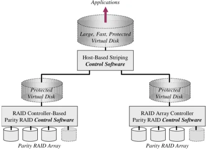
Host-based data striping is also particularly useful for aggregating the capacity and performance of the virtual disks instantiated by controller-based mirrored or parity RAID arrays.

RAID Array Controller Parity RAID Control Software

Parity RAID Array

RAID Controller-Based Parity RAID Control Software

Parity RAID Array Protected

Virtual Disk

Protected Virtual Disk

Host-Based Striping

Control Software Large, Fast, Protected

Virtual Disk Applications

Figure 10: Host-Based Striping of Controller-Based parity RAID Arrays

Figure 10 illustrates another application of data striping that is unique to host-based implementations. In many instances, it is beneficial to use host-based data striping to aggregate protected the virtual disks presented by RAID controllers into a single larger virtual disk for application use. The Large, Fast, Protected Virtual Disk pre-sented to applications by host-based control software in Figure 10 is a single block space that easier to manage, and will generally outperform two Protected Virtual

(21)

Disks presented individually. Host-based striping and mirroring control software can

be used in several similar circumstances to augment RAID controller capabilities.

Why Data Striping Works

Disk subsystem designers implement data striping to improve I/O performance. To understand why it works, one must appreciate that nearly all I/O intensive applica-tions fall into two broad categories:

➨ I/O request intensive. These applications typically perform some type of

trans-action processing, often using relational databases to manage their data. Their I/O requests tend to specify relatively small amounts of randomly addressed data. These applications usually consist of many concurrent execution threads, and thus many of their I/O requests are made without waiting for previous re-quests to be complete.

➨ data transfer intensive. These applications move long sequential streams of

data between application memory and storage. Scientific, engineering, graphics, and multimedia applications typically have this characteristic. I/O requests made by these applications typically specify large amounts of data, and are sometimes issued ahead of time (“double buffered”) to minimize idle time. Striping data across an array of disks improves the performance of both of these types of application, for different reasons. Some disk array subsystems allow the user to adjust the stripe depth to optimize for one type of application or the other.

Striping and I/O Request Intensive Applications

The performance of I/O request intensive applications is often limited by how fast disks can execute I/O requests. Today, a typical disk takes about 10 milliseconds to seek, rotate, and transfer data for a single small request (around 4K Bytes). The upper limit on the number of randomly addressed small requests such a disk can execute is therefore about 100 per second (1000 milliseconds in a second ÷ 10 milliseconds per request = 100 requests per second). Many server-class applications require

substan-tially more than this.

In principle, it is possible to split an application’s data into two or more files and store these on separate disks, thereby doubling the disk resources available to the applica-tion. In practice, however, there are two problems with this:

➨ It is awkward to implement, inflexible to use, and difficult to maintain.

➨ Application I/O requests do not necessarily split evenly across the disks.

So while dividing an application’s data into multiple files is sometimes done in very large applications, it is not a practical solution for most.

(22)

Data striping, on the other hand, does probabilistically balance such an application’s I/O requests evenly across its disk resources. To an application using a striped disk array, the entire array appears as one large disk. There is therefore no need to split data into multiple files.

Stripe 0

Stripe1 Record 000

Record 001 Record 002 Record 003 Record 004 Record 005 Record 006 Record 007

Record 007 Record 008 Record 009 Virtual Block 015

Virtual Block 004 Record 000 Record 001 Record 002

Record 003 Record 004 Record 005 Record 006

etc. Physical Disk C Application’s

view of file

Physical Data Layout

Record 008 Record 009

Figure 11: Effect of Data Striping on File Location

In the physical layout of data on the disks, however, the file will be split, as Figure 11 illustrates. Figure 11 shows a ten block file stored on a three disk striped array with a stripe depth of four blocks. To the application (and indeed, to all operating system, file system, and driver software components except array’s control software), the file appears to be laid out in consecutive disk blocks. In fact, however, the file’s records are spread across the three disks in the array.

If an application were to access this file randomly, with a uniform distribution of rec-ord numbers, about 30% of the requests would be executed by Disk A, 30% by Disk B, and 40% by Disk C. If the file were extended in place, the new records would be stored starting at Virtual Block 15, and then on Disk B, Disk C, and stripe 2 (not shown) of Disk A, and so forth. The larger a file, the more evenly its blocks are dis-tributed across a striped array’s disks.

Uniformly distributed requests for records in a large file will tend to be distributed uniformly across the disks, whether the array uses striped or contatenated mapping. The benefit of striping arises when request distribution is not uniform, as for example a batch program processing record updates in alphabetical order, which tends to cause relatively small segments of the file to be accessed frequently. Figure 12 illustrates this benefit.

(23)

Fry Frome Frederick Aaron Able Alpha Adelman Bates Carlton Farrell Feeney Disk A Fitzpatrick Franz Frederick Frizzell Frome Frugell Fry Frymoyer Disk B Harris Hart Jones Lambert Peterson Samuels Truestedt Young Disk C Application’s request stream Concatenated qrray: Most requests are directed to one disk

Fitzpatrick Farrell Stripe 0 Stripe1 Aaron Able Alpha Adelman Frome Frugell Fry Frymoyer Disk A Bates Carlton Farrell Feeney Harris Hart Jones Lambert Disk B Fitzpatrick Franz Frederick Frizzell Peterson Samuels Truestedt Young Disk C Striped array:

Requests are distributed across disks

Fry Frome

Frederick Fitzpatrick

Farrell

Figure 12: Effect of Data Striping on I/O Request Distribution

In the upper diagram of Figure 12, the large file is not striped across the disks. Most accesses to records for names beginning with the letter F are directed to Disk B, since that disk holds most of that segment of the file. Disks A and C remain nearly idle. With data striping, however, there is a natural distribution of accesses across all of the array’s disks, as the lower diagram of Figure 12 illustrates. Striping data across a disk array tends to use all of the disk resources simultaneously for higher throughput under most circumstances. Even if the application’s I/O pattern changes, the I/O request load remains balanced.

An important subtlety of I/O request intensive applications is that data striping does not improve the execution time of any single request. It improves the average

(24)

previous ones to finish processing. Data striping only improves performance for I/O request intensive applications if I/O requests overlap in time. This is different from the way in which data striping improves performance for data transfer intensive ap-plications.

Striping and Data Transfer Intensive Applications

With a data transfer intensive application, the goal is to move large blocks of data between memory and storage as quickly as possible. These applications’ data is al-most always sequential files that occupy many consecutive disk blocks.

If such an application uses one disk, then I/O performance is limited by how quickly the disk can read or write a large continuous block of data. Today’s disks typically transfer data at an average of 10-15 MBytes/second (disk interfaces like ATA and SCSI are capable of much higher speeds, but a disk can only deliver data as fast as a platter can rotate past a head.

If a data transfer intensive application uses a striped disk array, however, multiple disks cooperate to get the data transfer done faster. The data layout for a data transfer intensive application using the virtual disk presented by a three disk striped array is illustrated in Figure 13.

Stripe 0

Stripe1 Segment 000

Segment 001 Segment 002

Segment 017

Virtual Block 000 Virtual Block 001 Segment 000 Segment 001

Segment 010 Segment 011 Segment 012 Segment 013

etc. Disk A

etc. Disk B

Segment 018 Segment 019 Virtual Block 022 Virtual Block 023

etc. Disk C Application’s

view of data (e.g., video clip)

Physical Data Layout

Segment 018 Segment 019

• • •

Figure 13: Data Striping for Data Transfer Intensive Applications

The application illustrated in Figure 13 accesses a large file in consecutive segments.7

The segments have no meaning by themselves; they are simply a means for subdi-viding the file for buffer management purposes. When the application reads or writes this file, the entire file is transferred, and the faster the transfer occurs, the better. In

(25)

the extreme, the application might make one virtual disk request for the entire file. The disk array’s control software would translate this into:

1. A request to Disk A for Segments 000 and 001 2. A request to Disk B for Segments 002 through 005 3. A request to Disk C for Segments 006 through 009 4. A request to Disk A for Segments 010 through 013 5. A request to Disk B for Segments 014 through 017 6. A request to Disk C for Segments 018 and 019

Because the first three requests are addressed to different disks, they can execute si-multaneously. This reduces the data transfer time compared to transferring from a single disk. The control software can make the fourth request as soon as the first completes, the fifth as soon as the second completes, and the sixth as soon as the third completes. The overall data transfer time is about the time to transfer the eight seg-ments from Disk B, just a little over a third of the data transfer time for the entire file from one disk.

A Summary of the I/O Performance Effects of Data Striping

Figure 14 presents a qualitative summary of how a striped disk array performs rela-tive to a single disk. The icon at the center of the two dimensional graph represents performance that might be expected from a single disk. The other two icons represent how striped array performance compares to single disk performance.

Request Execution Time Throughput

(I/O Requests/Second)

Disk Small random reads and writes Large sequential

reads and writes

lower higher

fewer

more _{Striped Array} _{Striped Array}

Dotted lines represent typical single-disk

performance

(26)

Figure 14 has two dimensions because there are two important ways to measure I/O performance. One is throughput, how much work gets done per unit of time. The other is average execution time for individual requests (that does not include any time a request spends waiting to be executed).

The graph in Figure 14 indicates that for applications whose I/O consists of randomly addressed requests for small amounts of data, data striping improves throughput rela-tive to a single disk, but does not change the execution time of individual requests. Throughput improves because striping tends to balance the I/O requests across the disks, keeping them all “working.” Request execution time does not change because most requests are executed by one disk in both cases.

Even though request execution time does not change, data striping tends to reduce the time that requests have to wait for previous requests to finish before they can begin to execute. Thus, the user perception is that requests execute faster, because they spend less time waiting to start executing. Of course, if there is nothing to wait for, then a single request to a striped disk array will complete in about the same time as a similar request to a disk. The busier a striped array gets, the better it seems to perform, up to the point at which it is saturated (all of its disks are working at full speed).

Large sequential reads and writes also perform better with striped arrays. In this case, both throughput and request execution time are improved relative to a single disk. In-dividual request execution time is lower because data transfer, which accounts for most it, is done in parallel by some or all of the disks. Throughput is higher because each request takes less time to execute, so a stream of requests executes in a shorter time. In other words, more work gets done per unit time.

An Important Optimization: Gather Writing and Scatter Reading

Sophisticated disk subsystems can even combine requests for multiple data stripes into a single request, even though the data will be delivered to non-consecutive mem-ory addresses. Figure 15 illustrates this.

(27)

Segment 000 Segment 001 Segment 002

Segment 006

Virtual Block 000 Virtual Block 001 Segment 000 Segment 001 Segment 010 Segment 011 Segment 012 Segment 013 etc. Disk A Application memory

Disk A from Figure 11 Example Segment 007 Segment 008 Segment 003 Segment 004 Segment 005 Segment 009 Segment 010 Segment 011 Segment 012 Segment 013 Segment 000 Segment 001 Segment 002 Segment 006 Application memory) Segment 007 Segment 008 Segment 003 Segment 004 Segment 005 Segment 009 Segment 010 Segment 011 Segment 012 Segment 013 Segment 000 Segment 001 Segment 010 Segment 011 Segment 012 Segment 013 Segment 000 Segment 001 Segment 010 Segment 011 Segment 012 Segment 013 Gather writing Scatter reading etc.

Figure 15: Gather Writing and Scatter Reading

Figure 15 illustrates the Disk A of Figure 13. If the application writes the entire file at once, then Segments 000 and 001, and Segments 010 through 013 will be written to consecutive blocks on Disk A. Sophisticated disk subsystems include hardware that allows non-consecutive areas of application memory to be logically “gathered” so that they can be written to consecutive disk blocks with a single request. This is called

gather writing. These subsystems also support the converse capability—the delivery

of consecutive disk blocks to non-consecutive application memory areas as they are read from the disk. This is called scatter reading.

Scatter reading and gather writing improve performance by:

➨ eliminating at least half of the requests that control software must make to sat-isfy an application request, and,

➨ eliminating “missed” disk revolutions caused by the time required by control

software to issue these additional requests (e.g., requests 4-6 in the example of

Figure 13).

Scatter-gather capability is sometimes implemented by processor memory manage-ment units and sometimes by I/O interface ASICs.8_{It is therefore usually available to}

both host-based and controller-based RAID implementations.

Data Striping with Redundancy

The preceding examples have described a RAID Level 0 array, with data striped across the disks, but without any redundancy. While it enhances I/O performance, data striping also increases the impact of disk failure. If a disk in a striped array fails,

8 Application Specific Integrated Circuits, such as the single-chip SCSI and Fibre Channel interfaces found on some computer mainboards.

(28)

there is no reasonable way to recover any of the files striped across it. One disk fail-ure results in loss of all the data stored on the array. Therefore, when data is striped across arrays of disks to improve performance, it becomes crucial to protect it against disk failure. Data striping and data redundancy are a natural match. Figure 16 illus-trates how a striped disk array can be augmented with a “parity disk” for data redun-dancy. This is the check data layout that defined RAID Levels 3 and 4 in A Case for

Redundant Arrays of Inexpensive Disks.

Stripe 0

etc. Disk A

etc. Disk B

etc. Disk C

000 ⊕ 004 ⊕ 008 001 ⊕ 005 ⊕ 009 002 ⊕ 006 ⊕ 010 003 ⊕ 007 ⊕ 011 012 ⊕ 016 ⊕ 020 013 ⊕ 017 ⊕ 021 014 ⊕ 018 ⊕ 022 015 ⊕ 019 ⊕ 023

etc. Disk D

(parity)

Figure 16: Data Striping with Parity RAID

Disk D in Figure 16 holds no user data. All of its blocks are used to store the exclu-sive OR parity of the corresponding blocks on the array’s other three disks. Thus, Block 000 of Disk D contains the bit-by-bit exclusive OR of the contents of Virtual Blocks 000, 004, and 008, and so forth. The array depicted in Figure 16 offers the data protection of RAID and the performance benefits of striping…almost.

Writing Data to a RAID Array

RAID “works” because the parity block represents the exclusive OR of the corre-sponding data blocks, as illustrated in Figure 6 and Figure 7. But each time an appli-cation writes data to a virtual disk block, the parity that protects that block becomes invalid, and must be updated. Assume, for example, that an application writes Virtual Disk Block 012 in the array illustrated in Figure 16. The corresponding parity block on Disk D must be changed from

(old) Block 012 contents ⊕ Block 016 contents ⊕ Block 20 contents

to

(new) Block 012 contents ⊕ Block 016 contents ⊕ Block 20 contents

In other words, when an application writes Virtual Disk Block 012, the RAID array’s

control software must:

➨ Read the contents of Virtual Disk Block 012 into an internal buffer,

(29)

➨ Compute the exclusive OR of Virtual Disk Blocks 016 and 020,

➨ Compute the exclusive OR of the above result with the (new) contents for Vir-tual Disk Block 012,

➨ Make a log entry, either in non-volatile memory or on a disk, indicating that data is being updated,

➨ Write the new contents of Virtual Disk Block 012 to Disk A,

➨ Write the new parity check data to Disk D,

Make a further log entry, indicating that the update is complete. Figure 17 illustrates the reads and writes to the array’s disks required by a single application write request.

Stripe 0

(old)Virtual Block 012 Virtual Block 013 Virtual Block 014 Virtual Block 015

etc. Disk A

etc. Disk B

etc. Disk C

000 ⊕ 004 ⊕ 008 001 ⊕ 005 ⊕ 009 002 ⊕ 006 ⊕ 010 003 ⊕ 007 ⊕ 011 012 ⊕ 016 ⊕ 020 013 ⊕ 017 ⊕ 021 014 ⊕ 018 ⊕ 022 015 ⊕ 019 ⊕ 023

etc. Disk D

(parity)

Control Software computes

⊕

Virtual Block 016 Virtual Block 020

⊕

(new)Virtual Block 012

Control Software writes (new)Virtual Block 012

Application writes:

Control Software reads

Figure 17: One Write Algorithm for a Parity RAID Array

An Important Optimization for Small Writes

A useful property of the exclusive OR function is that adding the same number to an exclusive OR sum twice is the same as not adding it at all. This can easily be seen by observing that the exclusive OR of a binary number with itself is zero. This can be used to simplify RAID parity computations by observing that:

(old) Block 012 contents ⊕ (old)parity

is the same as:

(old) Block 012 contents ⊕[(old) Block 012 contents ⊕ Block 016 contents ⊕ Block 20 contents]

or:

[(old) Block 012 contents ⊕ (old) Block 012 contents]⊕ Block 016 contents ⊕ Block 20 contents

(30)

Block 016 contents ⊕ Block 20 contents.

In other words, the exclusive OR of the data to be replaced with the corresponding parity is equal to the exclusive OR of the other corresponding user data blocks in the array. This is true no matter how many disks are in the array.

This property leads to an alternate technique for updating parity. The control

soft-ware:

➨ reads the data block to be replaced,

➨ reads the corresponding parity block, and,

➨ computes the exclusive OR of the two.

These steps eliminate the “old” data’s contribution to the parity, but leave all other blocks’ contributions intact. Computing the exclusive OR of this result with the “new” data written by the application gives the correct parity for the newly written data. Using this technique, it is never necessary to access more than two disks (the disk to which application data is to be written and the disk containing the parity) for a single-block application write. The sequence of steps for updating Block 012 (Figure 16) is:

➨ Read the contents of Virtual Disk Block 012 into an internal buffer,

➨ Read the contents of the corresponding parity block on Disk D into an internal buffer,

➨ Compute the exclusive OR of the two blocks just read,

➨ Compute the exclusive OR of the above result with the (new) contents for Vir-tual Disk Block 012,

➨ Make a log entry, either in non-volatile memory or on a disk, indicating that data is being updated,

➨ Write the new contents of Virtual Disk Block 012 to Disk A,

➨ Write the new parity check data to Disk D,

➨ Make a further log entry, indicating that the update is complete.

The number of read, write, and computation steps using this algorithm is identical to that in the preceding example. For arrays with five or more disks, however, this algo-rithm is preferable, because it never requires accessing more than two of the array’s disks, whereas the preceding algorithm would require that all of the user data disks unmodified by the application’s write be read. This algorithm is therefore the one that is implemented in parity RAID control software.9

9 These examples deal with the case of an application write of a single block, which always maps to one disk in a parity RAID array. The same algorithms are valid for application writes of any number of consecutive blocks that map to a single disk. More complicated scenarios arise when an application write maps to blocks on two or more disks.

(31)

Stripe 0 Virtual Block 000

(old)Virtual Block 012 Virtual Block 013 Virtual Block 014 Virtual Block 015

etc. Disk A

etc. Disk B

etc. Disk C

000 ⊕ 004 ⊕ 008 001 ⊕ 005 ⊕ 009 002 ⊕ 006 ⊕ 010 003 ⊕ 007 ⊕ 011 012 ⊕ 016 ⊕ 020 013 ⊕ 017 ⊕ 021 014 ⊕ 018 ⊕ 022 015 ⊕ 019 ⊕ 023

etc. Disk D

(parity)

Control Software computes

⊕

(old)Virtual Block 012

012 ⊕ 016 ⊕ 020

⊕

(new)Virtual Block 012

Control Software writes (new)Virtual Block 012

Application writes:

Control Software reads

Figure 18: Optimized Write Algorithm for a Parity RAID Array

An Important Optimization for Large Writes

The preceding discussion dealt with application write requests that modify data on a single disk. If an application makes a large write request, then it is possible that all of the data in a stripe will be overwritten. In Figure 16, for example, an application re-quest to write Virtual Disk Blocks 12-23, would cause all the user data in a stripe to be overwritten.

When an application write results in all the data in a stripe being written, then “new” parity can be computed entirely from data supplied by the application. There is no need for the control software to perform “extra” disk reads. Once parity has been computed, the entire stripe, including data and parity, can be written in parallel. This results in a speedup, because the long data transfer is divided into parts, and the parts execute in parallel, as with the striped array in the example of Figure 13.

Even with these optimizations, the “extra” computation and I/O requred by RAID up-date algorithms takes time and consumes resources. Many users deemed early RAID subsystems unusable because of this “write penalty.” Today, the write penalty has largely been hidden from applications through the use of non-volatile cache memory, at least in controller-based RAID implementations.10_{In either case, with applications}

that do a lot of writing it is still possible to distinguish between the performance of a disk or striped array and the performance of a parity RAID array.

10 Non-volatile memory is not usually available to host-based RAID implementations, so it is more difficult to mask the write penalty with these. For this reason, mirroring and striping are generally preferable techniques for host-based RAID.

(32)

The Parity Disk Bottleneck

With a perfectly balanced I/O load of overlapping application write requests to Disks A, B, and C in the array depicted in Figure 16 (the goal of data striping), there is a natural bottleneck. Each of the application write requests causes the array’s control

software to go through a set of steps similar to those listed on page 30. In particular,

while data writes are distributed, every application write requires that the control

software write some block(s) on Disk D (the “parity” disk). The parity disk is the

ar-ray’s write performance limitation. Writes cannot proceed at a rate any greater than about half the speed with which the parity disk can execute I/O requests.

This bottleneck was discerned by early RAID researchers, who devised a means of balancing the parity I/O load across all of the array’s disks. They simply interleaved the parity with the striped data, distributing parity as well as data across all disks. Figure 19 illustrates a RAID array with data striping and interleaved parity.

Stripe 0

etc. Disk A

etc. Disk B

etc. Disk C

000⊕ 004⊕008 001⊕ 005⊕009 002⊕ 006⊕010 003⊕ 007⊕011 012⊕ 016⊕020

013⊕ 017⊕021 014⊕ 018⊕022 015⊕ 019⊕023

etc. Disk D

(parity)

Stripe 2

Virtual Block 044 Virtual Block 045 Virtual Block 046 Virtual Block 047 Virtual Block 028 Virtual Block 029 Virtual Block 030 Virtual Block 031

Virtual Block 040 Virtual Block 041 Virtual Block 042 Virtual Block 043 024⊕ 028⊕032

025⊕ 029⊕033 026⊕ 030⊕034 027⊕ 031⊕035 036⊕ 040⊕044

037⊕ 041⊕045 038⊕ 042⊕046 039⊕ 043⊕047

Figure 19: RAID Array with Data Striping and Interleaved Parity

Figure 19 illustrates a RAID array with both data striping and interleaved parity. The concept of parity interleaving is simple. The parity blocks for the first data stripe are stored on the “rightmost” disk of the array. The parity blocks for the second stripe are stored on the disk to its left, and so forth. In the example of Figure 19, the parity blocks for Stripe 4 would be stored on Disk D.

Distributing the RAID parity across all of the array’s disks balances the “overhead” I/O load caused by the need to update parity. All of the “extra” reads and writes de-scribed above must still occur, but the ones that update parity are no longer

(33)

concen-trated on a single disk. In the best case, an array with interleaved parity can execute random application write requests at about one fourth the speed of all the disks in the array combined.

With or without a cache to mask the effect of writing, interleaved parity makes arrays perform better, and so most of the arrays in use today use this technique. The combi-nation of interleaved parity check data and data striping was called RAID Level 5 in

A Case for Redundant Arrays of Inexpensive Disks. The 5 does not refer to the

number of disks in the array as is sometimes thought. RAID Level 5 arrays with as few as three and as many as 20 disks have been implemented. Typically, however, RAID Level 5 arrays contain between four and ten disks as illustrated in Figure 4.

A Summary of Parity RAID Performance

Figure 20 summarizes the performance of parity RAID arrays relative to that of an equivalent single disk. This summary reflects only disk and controller operations, and not the effect of write-back cache or other performance optimizations.

Request Execution Time Throughput

(I/O Requests/Second)

disk Small reads Large reads

lower higher

fewer more

Large writes

Small writes

parity RAID parity RAID

Figure 20: Relative Performance of Parity RAID Arrays

As Figure 20 indicates, a parity RAID typically performs both large sequential and small random read requests at a higher rate than a single disk. This is due to the load balancing that comes from striping of data across the disks as described in the exam-ple of Figure 13. When writing, there is fundamentally more work to be done, how-ever, as described on page 30. A parity RAID array therefore completes requests more slowly than a single disk. For large writes (for example, and entire stripe of data), this penalty can be mitigated by pre-computing parity as described on page 31.