Thesis

IMPACT OF SEA LEVEL RISE ON DEVELOPMENT SUITABILITY IN NEW YORK CITY

By Marisa Berry

Honors Thesis

Curriculum for the Environment and Ecology University of North Carolina at Chapel Hill

April 23, 2014

Approved:

Abstract

Global climate change and resultant rising sea levels and more frequent flooding are impacting the sustainability and vitality of coastal communities, making identifying vulnerable areas particularly important. Sea level rise projections for the 2020s and 2050s were

incorporated into a land use suitability analysis of New York City, which was conducted in a GIS environment based on Ian McHarg’s overlay methods. The analytical hierarchy process (AHP) was used to produce weights for the six criteria considered, which were then reclassified and combined according to a weighted linear combination. The results of the suitability analysis suggest that Eastern Staten Island and the southern shore of Brooklyn and Queens are

particularly unsuitable for future development. This analysis could be improved by better considering hydrological connectivity when modeling sea level rise.

Introduction

of areas suitable for urbanization and development based on a set of environmental criteria. Including sea level rise as a criterion in the suitability analysis introduces a temporal element that considers how suitability will change in response to global change and will make suitability analysis a more informative tool for decision makers.

I will first review the overarching issues of climate change, sea level rise, New York City’s particular vulnerability to sea level rise, and the city’s current patterns of development before providing a review of the literature on suitability analysis. I will then detail the data and methods used before discussing the results and implications of this analysis.

Background

Climate Change, Sea Level Rise, and Coastal Vulnerability

The IPCC (2007) predicts global sea levels to rise between 0.18 and 0.59m by 2100, although more recent studies provide evidence for a rise of over a meter in the same period of time (Rahmstorf et al. 2007; U.S. Army Corps of Engineers 2011; Scientific Committee on Antarctic Research 2009; Arctic Monitoring and Assessment Programme 2011; Vellinga et al. 2009). Rising sea levels are associated with more frequent acute weather events, such as typhoons and hurricanes, storm surges, and higher levels of precipitation (Balk et al. 2009; FitzGerald et al. 2008). Additionally, there is a high degree of uncertainty associated with these predictions, making planning for sea level rise and more extreme weather events challenging (Meo 1990).

beaches and barrier islands (London and Volonte 1991; FitzGerald et al., 2008). The changing topography and more frequent extreme weather events will, in turn, impact coastal communities and their ability to weather storms.

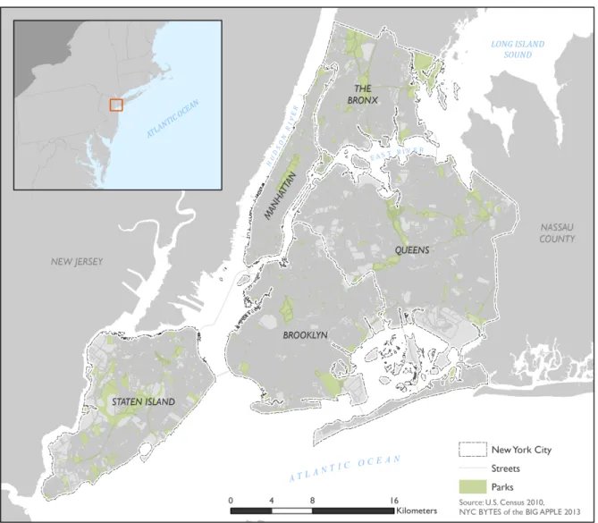
Study Area Figure 1. Study Area

global as average temperatures continue to increase. While global sea levels are projected to rise by 0.35 meters, it is expected that sea levels in the New York City region will rise 0.23 to 1.07 meters by 2100 (IPCC 2007; Bloomfield 1999). According to the New York City Panel on Climate Change (2013), middle range estimates place sea level rise are 0.10 to 0.20 meters in the 2020s and 0.28 to 0.61 meters in the 2050s.

In the fall of 2012, Hurricane Sandy served as a reminder to the area’s vulnerability. The storm’s aftermath presented the region with many challenges, as is the case with most natural disasters of comparable scale. After such an extreme event, infrastructure is wrecked, business activity is interrupted, and people migrate away from the impacted area (Ewing et al. 2007; Thompson 2009). The National Hurricane Center estimates Hurricane Sandy resulted in over $50 billion in damage (NOAA 2013).

Development Patterns and Policies

Before performing a suitability analysis, it is important to consider current and anticipated development patterns within the study area. While this analysis will consider

environmental factors, the natural environment is shaped by the policies governing development. New York City is intensifying development along certain portions of the waterfront, while also restoring the ecological integrity of other areas. There has been continuous redevelopment along the waterfront (Buttenwieser 1999). With PlaNYC: A Greener, Greater New York, the

Bloomberg administration accelerated waterfront redevelopment but also cited as a priority the city’s improved resilience to a changing climate (City of New York 2011). The study Urban Waterfront Adaptive Strategies identifies a variety of approaches for the City to take in adapting to threats associated with climate change and promoting coastal climate resilience (NYC

Department of City Planning 2013b). After Hurricane Sandy, the City unveiled the plan A Stronger, More Resilient New York, which outlines its approach to rebuilding post-Sandy and preventing another event comparable to Sandy from happening again (NYC Department of City Planning 2013a). All of these plans provide the City with a framework for waterfront

development.

Recent changes in flood zoning policy will also inform future development. The Federal Emergency Management Agency (FEMA) is expanding the flood zones designated in Flood Insurance Rate Maps (FIRMs) and flood elevations. This is in addition to the changes in the New York State Building Code adopted in January 2013 requiring building protections for one to two feet higher than FEMA flood levels (NYC City Planning Commission 2013). As a result of changes in the federal and state policy, more buildings will be designated within the flood zone and required to have the appropriate protections. In response, the New York City Council passed the Flood Resilience Zoning Text Amendment to allow for building construction based on the most recent FIRMs (NYC City Planning Commission 2013; Aerts and Botzen 2011). These federal, state and local policies are informing development in flood zones, and it is within this context that I will consider the future development suitability in New York City.

Suitability analysis: an overview

This study will use a land suitability analysis to identify areas best suited for urbanization with a particular interest as to how suitability change when considering rising sea levels. If in determining future land use decision makers employ suitability analysis, then it is logical to consider future conditions. The results of a suitability analysis today may be different from those fifty years from now simply because the processes which regulate the criteria considered in a suitability analysis are dynamic.

A GIS-based land suitability analysis can be used to determine land uses most

biological processes,” and he used that principle to develop the ecological inventory process through mapping overlay technique (1969, p. 104). Since the publication of McHarg’s Design with Nature, methods for suitability analysis have evolved and today it is used for a variety of applications, including but not limited to: geological favorability, agriculture, site selection, habitat for animal and plant species, and environmental impact assessment (Malczewski 2004).

There are three general methods to perform a suitability analysis: computer-assisted overlay mapping, multi-criteria evaluation, and artificial intelligence (Chakma 2014; Malczewski 2004). Elements of the three methods are often blended in practice, and some form of overlay mapping is used in most methods. Computer-assisted overlay mapping is the next step in the evolution of the manual overlay mapping method. It is commonly applied through Boolean operation and weighted linear combination (WLC). This method is easy to implement in a GIS environment, but is often used without a full understanding of the underlying assumptions (the weights assigned to each criteria). The overlay mapping method is insufficient by itself because it assumes all attributes to be linearly independent (Hopkins 1977). Boolean operations and WLC may oversimplify land use planning by excluding any consideration for value judgments and only focusing on facts. Value judgments can be incorporated through multi-criteria decision making (MCDM) methods.

There has been substantial research on the topic of the integration between GIS and MCDM and is a widespread approach to suitability analysis (Yu et al. 2009; Malczewski 2006). MCDM methods apply both spatial and non-spatial data to decision making and are divided between multi-objective methods and multi-attribute methods (Malczewski 2004). Multiattribute methods are data-oriented, whereas multi-objective methods are based on mathematical

their ability to incorporate both qualitative and quantitative criteria (Greene et al. 2011). As a result of their relative ease, multi-attribute methods are more commonly used in solving land-suitability problems. The analytical hierarchy process (AHP), developed by Saaty (1980), is a widely used multi-attribute technique used to obtain the weights for each suitability criteria. It is regularly integrated into GIS-based suitability analysis because the AHP makes it relatively easy to derive criteria’s weights, one of the problems associated with MCDM (Saaty 1980; Saaty and Vargas 1991).

There are a number of problems associated with MCDM methods. First, multi-attribute methods do not solve the problem of assumed linearity among attributes that also plagues the overlay method. Second, the MCDM method assumes the input data to be accurate when in reality the data will have some associated degree of inaccuracy and uncertainty. Using a multi-criteria evaluation method in land suitability analysis has the potential to overlook the

complexities of the systems underlying land use planning (Yu et al. 2011). While the AHP is a widely used approach, there are other methods that might produce different results, and the inconsistency between methods is an additional problem with MCDM.

Finally, artificial intelligence (AI) methods address data inaccuracies and uncertainties by allowing for vagueness and uncertainty (Cheng et al. 2001). AI methods include fuzzy logic techniques, neural networks, evolutionary algorithms, and cellular automata. Fuzzy logic is an AI method particularly appropriate for addressing the uncertainty of spatial boundaries

methods, but their complexity limits their application and renders them inaccessible to many city planners and policymakers (Malczewski 2004). Additionally, they are less easily integrated into a GIS environment and many AI methods’ internal processes are hidden. This lack of

transparency makes their results less likely to be considered by decision makers (O’Sullivan and Unwin 2003).

This study will apply MCDM methods through the AHP and weighted linear combination to determine how sea level rise will influence land uses. MCDM methods are preferred because of their ability to incorporate value judgments and because they are able to consider both qualitative and quantitative criteria (Malczewski 2006; Greene et al. 2011). The AHP will be used to calculate criteria weights because of its ability to objectively compare and rank

Methodology

Evaluation Criteria

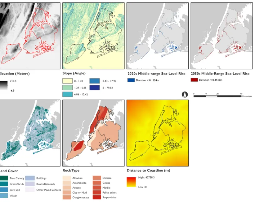
Evaluation criteria should be chosen so that they offer a comprehensive understanding of the problem, and were selected based on a review of similar studies (Saaty and Vargas 2001; Malczewski 1999; Chen et al. 2009). The following criteria will be used: land cover; elevation; slope; rock type; distance to coastline; and areas inundated from sea level rise (Table 1, Fig. 2).

Table 1. Data Sources

Evaluation Criteria Source Citation

Land Cover University of Vermont Spatial Analysis Laboratory & New York City Urban Field Station (2010)

Rojas, Pino & Jacque 2013; Pathan et al. 1992; Chakma 2013; Doygun et al. 2008; Dong et al. 2008; Reshmidevi et al. 2009; Yu et al. 2011

Elevation US Geological Survey (2013) Chakma 2013; Dong et al. 2008; _{Reshmidevi et al. 2009}

Slope Derived from DEM (USGS 2013). Joerin et al. 2001; Davidson et al. 1994; Aly _{et al. 2005; Pourebrahim et. Al. 2011}

Rock Type USGS (2008) Davidson et al. 1994; Yu et al. 2009; Pathan _{et al. 1992; Reshmidevi et al. 2009} Distance to

Modeling Inundation

Inundated areas will be modeled by applying sea-level rise projections from the NYC Panel on Climate Change (2013) to the bathtub model approach (Poulter and Haplin 2008; Gesch 2009). This method assumes that sea-level rise will be evenly distributed and sea levels will rise as if filling up a bathtub. This is an elementary approach, as sea level rise will not be uniform across a region and will be influenced by changing landscape morphology and ecological feedbacks (Poulter and Haplin 2008).

A land cell is considered inundated if it meets two conditions: its elevation is lower than that of the considered sea level rise projection, and it is connected to the ocean via a continuous path of other inundated cells (Gesch 2009; Poulter and Halpin 2007; Bales et al. 2007). The second condition considers the hydrological connectivity of the land cell; otherwise, isolated inland land cells meeting the elevation threshold would be included. The averages of the middle range estimates are used in this analysis (Table 2).

Table 2. Sea Level Rise Projections

Baseline (2000-2004) 0 meters Middle range (25th to 75th percentile) Average

2020s 0.1016m to 0.2032m 0.1524m

2050s 0.2794m to 0.6096m 0.4445m

Analytical Hierarchy Process and Weighted Linear Combination

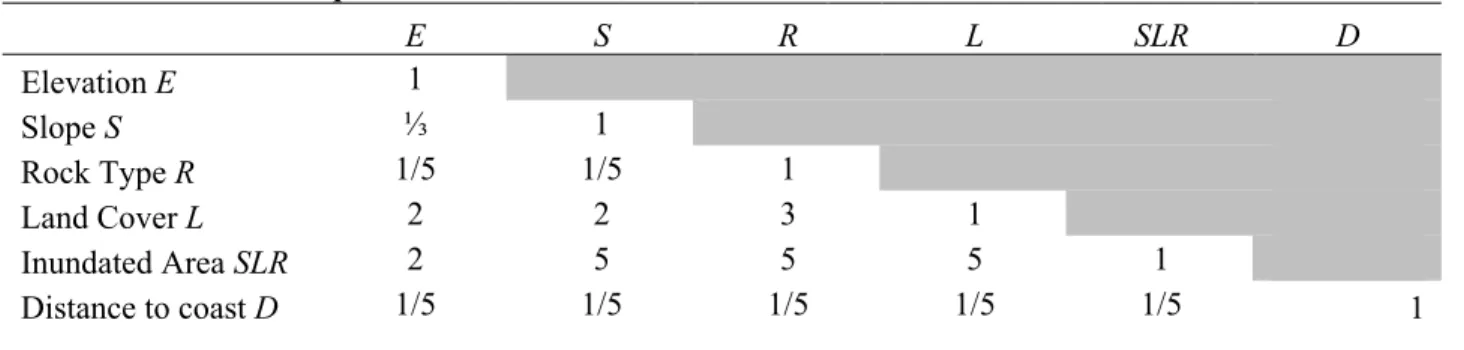
The criteria considered are not measured according to the same scale, and land cover and lithology are categorical. In order to combine criteria, the different scales are reconciled by establishing priorities through pairwise comparisons. The AHP uses a “fundamental scale” of 1-9; it is fundamental in that has been evaluated for effectiveness and is based on

stimulus-response theory (Saaty and Vargas 2001; Saaty 2001). The values of 1-9 (or, alternatively, their inverses) are assigned to each pair of criteria to establish their importance relative to one another. One refers to the pair of criteria being of equal importance, while 9 refers to the criterion being of extreme importance relative to the other criterion being compared. The resultant inverse matrix (Table 3) details each pairwise comparison and their relative priorities.

An advantage of the pairwise method is that only two criteria are considered at a time, eliminating the need to rank all of the criteria relative to each other at once (Malczewski 1999). Additionally, pairwise comparisons are better suited to situations in which “the accuracy and theoretical foundations are the main concerns (Malczewski 1999, p. 189).”

Table 3. Pairwise Comparison Matrix

E S R L SLR D

Elevation E 1

Slope S ⅓ 1

Rock Type R 1/5 1/5 1

Land Cover L 2 2 3 1

Inundated Area SLR 2 5 5 5 1

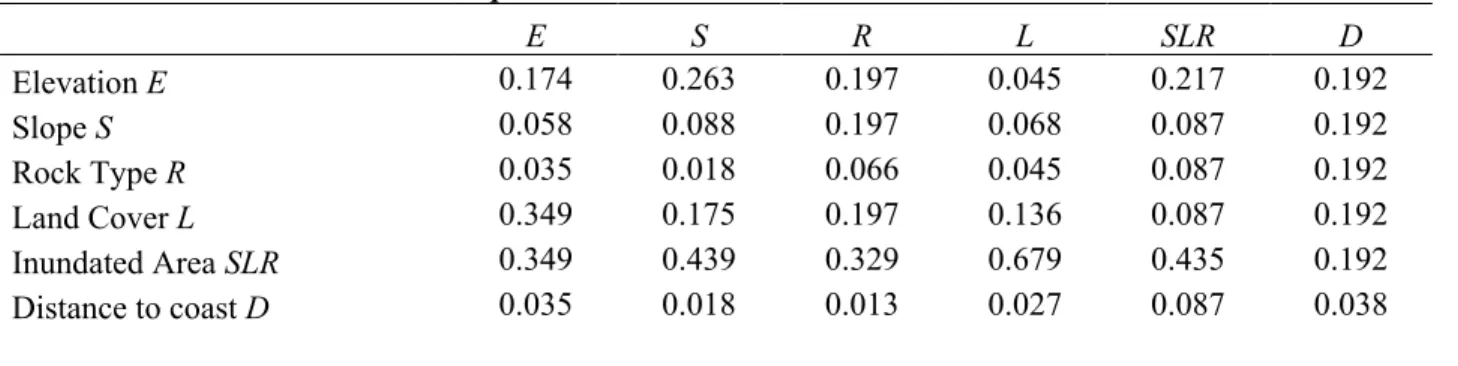
Table 4. Normalized Pairwise Comparison

E S R L SLR D

Elevation E 0.174 0.263 0.197 0.045 0.217 0.192

Slope S 0.058 0.088 0.197 0.068 0.087 0.192

Rock Type R 0.035 0.018 0.066 0.045 0.087 0.192

Land Cover L 0.349 0.175 0.197 0.136 0.087 0.192

Inundated Area SLR 0.349 0.439 0.329 0.679 0.435 0.192

Distance to coast D 0.035 0.018 0.013 0.027 0.087 0.038

The criterion weights are derived from the normalized pairwise comparison matrix (Table 4). The elements of the Eigenvector that corresponds to the maximum Eigenvalue of the normalized pairwise comparison matrix represent the criteria weights (Saaty and Vargas 2001; Feizizadeh and Blaschke 2012). An Eigenvector v is a nonzero vector that when multiplied by a matrix M

results in a vector that is parallel to v or equal to zero: Mv = λv, where λ is the Eigenvalue, a

scalar, associated with a given Eigenvector (Kuttler 2012).

Each criterion weight wi is the sum of a column in the normalized matrix divided by the sum of all of the normalized matrix elements bij. The weights are calculated as such:

The consistencies of priorities established in the pairwise comparison matrix are evaluated through the consistency ratio. A pairwise comparison matrix is considered consistent if the consistency ratio (CR) is less than 0.10 while a value greater than 0.10 suggests that the value judgments are inconsistent with each other and should be reevaluated (Saaty and Vargas 2001).

€

wi =

bij j=1 n

∑

bij j=1 n

∑

The CR is calculated as:

where CI is is the Consistency Index and RI is the Random Index, the consistency index of a

completely random comparison matrix. The RI associated with 6 criteria is 1.24. The

consistency index (CI) is found as:

where n is the number of criteria, and λmax is the Eigenvector associated with the comparison

matrix’s largest Eigenvalue. The consistency ratio associated with this pairwise comparison

matrix is 0.09; the pairwise comparisons are consistent and the resulting weights are appropriate

for a weighted linear combination.

In order to perform a weighted linear combination, the criteria’s heterogeneous

measurement scales and units were reconciled with each other by reclassifying their values

(Greene et al. 2011; Malczewski 2004). The criteria were reclassified into a scale of 0 to 4, with

4 representing the most suitable alternative (Fig 3; Table 5). The divisions of a criterion’s classes

were established at the natural breaks according to the Jenks Method, which minimizes statistical

variation within each class (Baz et al. 2009; Jenks 1977). As land cover and rock type are

qualitative criteria, they were reclassified according to standards in the literature (Afrouz 1992;

Djuric et al. 2013). Sea level rise was only reclassified into a binary scale, with 1 representing

no inundation and 0 representing inundation.

€

CR=CI

RI

€

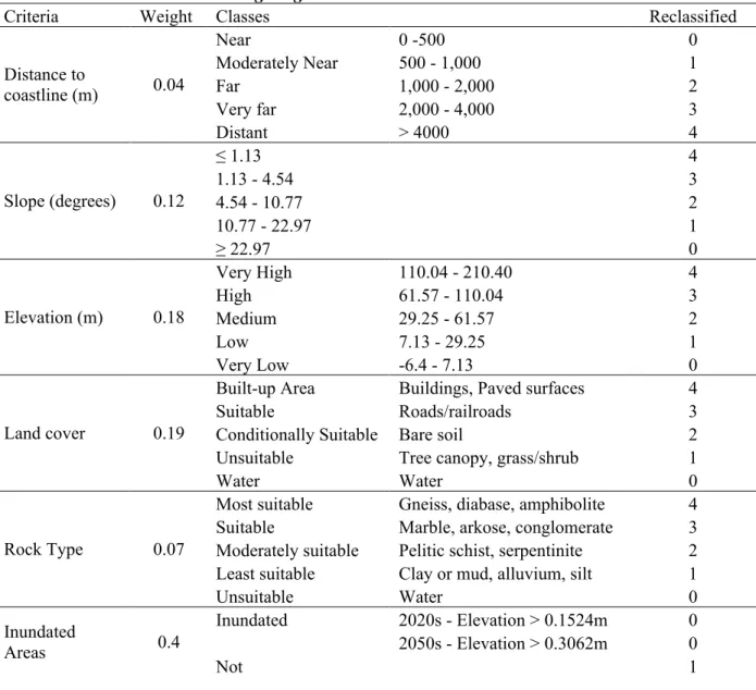
Table 5. Criteria Classes and Weighting

Criteria Weight Classes Reclassified

Near 0 -500 0

Moderately Near 500 - 1,000 1

Far 1,000 - 2,000 2

Very far 2,000 - 4,000 3

Distance to

coastline (m) 0.04

Distant > 4000 4

≤ 1.13 4

1.13 - 4.54 3

4.54 - 10.77 2

10.77 - 22.97 1

Slope (degrees) 0.12

≥ 22.97 0

Very High 110.04 - 210.40 4

High 61.57 - 110.04 3

Medium 29.25 - 61.57 2

Low 7.13 - 29.25 1

Elevation (m) 0.18

Very Low -6.4 - 7.13 0

Built-up Area Buildings, Paved surfaces 4

Suitable Roads/railroads 3

Conditionally Suitable Bare soil 2

Unsuitable Tree canopy, grass/shrub 1 Land cover 0.19

Water Water 0

Most suitable Gneiss, diabase, amphibolite 4 Suitable Marble, arkose, conglomerate 3 Moderately suitable Pelitic schist, serpentinite 2 Least suitable Clay or mud, alluvium, silt 1 Rock Type 0.07

Unsuitable Water 0

Inundated 2020s - Elevation > 0.1524m 0 2050s - Elevation > 0.3062m 0 Inundated

Areas 0.4

A weighted linear combination produced the final suitability score. The reclassified criteria were

weighted according to the weights generated by the AHP and then summed using the map

algebra tool in ArcGIS 10.1. The resultant number is a numeric representation of the land cell’s

suitability. In order to make the results more easily communicated, the final suitability scores

were then reclassified at their natural breaks according the Jenks Method. The final suitability

classes include: Most Suitable, Suitable, Conditionally Suitable, Moderately Suitable, and Not

Suitable.

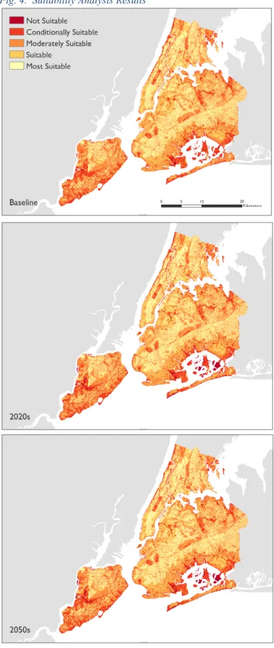
Results

Suitability maps for the baseline conditions and sea level rise projections for the 2020s and

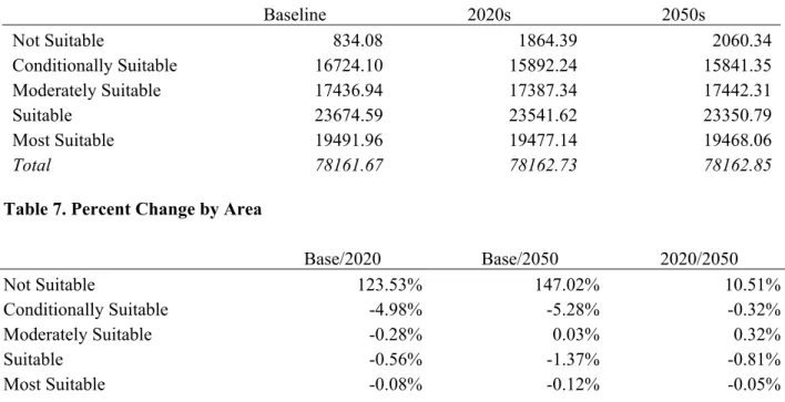
2050s were created (Fig. 4; Table 6; Table 7). The area classified as Not Suitable increased for

both the 2020s and 2050s, while Conditionally Suitable, Suitable, and Most Suitable decreased

for both time periods. The Moderately Suitable areas decreased between the baseline conditions

and the 2020s, but slightly increased between the 2020s and the 2050s.

Table 6. Suitability Classes by Area (Hectares)

Baseline 2020s 2050s

Not Suitable 834.08 1864.39 2060.34

Conditionally Suitable 16724.10 15892.24 15841.35

Moderately Suitable 17436.94 17387.34 17442.31

Suitable 23674.59 23541.62 23350.79

Most Suitable 19491.96 19477.14 19468.06

Total 78161.67 78162.73 78162.85

Table 7. Percent Change by Area

Base/2020 Base/2050 2020/2050

Not Suitable 123.53% 147.02% 10.51%

Conditionally Suitable -4.98% -5.28% -0.32%

Moderately Suitable -0.28% 0.03% 0.32%

Suitable -0.56% -1.37% -0.81%

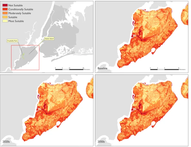
The areas with the most visible changes in suitability are eastern Staten Island (Fig. 6) and the

southern portions of Brooklyn and Queens, particularly Rockaway Peninsula and Jamaica Bay

(Fig. 5). Staten Island and Rockaway Peninsula act as New York City’s initial barriers to storms

moving in from the Atlantic Ocean. In the Rockaways, the peninsula separating Jamaica Bay

from the Atlantic Ocean, there was a significant decrease in suitable areas between the baseline

conditions and the 2020s. There was little significant change between the 2020s and 2050s for

the Rockaways. On Staten Island, the Not Suitable area increased most significantly on the

western edge bordering New Jersey in Freshkills Park along with the eastern side adjacent to

New York Bay. The impact of sea level rise on Staten Island’s eastern side is likely understated

Discussion

We can compare the areas affected by Hurricane Sandy with the results of this suitability

analysis (Fig. 7; Table 8). This analysis characterizes the extent of the one meter storm surge

during Hurricane Sandy as predominantly Conditionally Suitable, Moderately Suitable, and

Suitable. The storm surge extent has a larger area classified as Not Suitable when compared with

the city as a whole for both the 2020s and 2050s suitability analysis. For the entire city, the area

classified as Not Suitable was 2.38% and 2.64% for the 2020s and 2050s projections

respectively. However, within the storm surge extent, it is 3.66% for the 2020s and 4.81% for

the 2050s.

Table 8. Comparison of Suitability Analysis Results with Hurricane Sandy 1m Storm Surge Extent

Area (Hectares)

Percentage of Storm Surge Extent Area

2020s 2050s 2020s 2050s

Not Suitable 436.088 573.06 3.66% 4.81%

Conditionally Suitable 4649.34 4625.62 38.99% 38.79%

Moderately Suitable 2416.15 2463.07 20.26% 20.65%

Suitable 4004.78 3852.14 33.58% 32.30%

Most Suitable 419.11 411.67 3.51% 3.45%

That this suitability analysis characterizes the Hurricane Sandy storm surge extent as less

suitable than the rest of the city suggests this analysis provides results that reflect current

There are several limitations to this analysis. It is dependent on the accuracy of sea level rise

projections, and there is uncertainty associated with all climate models. The bathtub model

assumes that sea-level rise will be uniform across the region, when it will really be subject to

more local conditions. A more accurate model of sea level rise would account for bathymetry,

tidal patterns, and coastal geomorphology, among other factors. The distance to the shoreline

was used in combination with inundated areas as a proxy for flood and storm surge risk.

Incorporating floodplain areas and giving weight to areas more likely to flood would further

improve this analysis.

The biggest limitation with this suitability analysis is that it fails to fully consider the

relation between sea level rise and the adjacent areas. The only changes in suitability came in

the inundated areas, but rising sea levels and a changing coastline will have an impact beyond

them. For example, there was a limited change in suitability in Lower Manhattan. However,

based on previous flooding events, it’s evident that this area is much less suitable for

development than this analysis suggests. In future analysis, this disconnected could be remedied

by incorporating fuzzy logic techniques. Doing such would allow the inundated areas to have

more of an influence on the adjacent areas, whereas in this suitability analysis they were to a

certain degree treated independently.

One of the goals of this analysis was to examine how a changing condition – sea level

rise – impacts the suitability for future development. It assumes that the other conditions are

static; in reality they are dynamic and will not be the same in the observed time span. Criteria

are subject to both environmental and human forces. Unless there are significant human impacts,

the rock type, elevation, and slope will be largely the same given they change on a geologic time

therefore it is important to consider the results of this analysis within the context of current and

future patterns of development. In New York City, there has been a focus on waterfront

development, but this analysis does not consider how that development is adapted to withstand

environmental factors. This analysis could be improved by incorporating more detailed

information about the type of protections and adaptations used in a given building.

Another goal of this analysis was to provide a potential tool to urban planners,

developers, and policymakers regarding future development. While some areas are clearly

dominated by a single suitability class, other areas are a mix of two or three classes. These

mixed areas would make it difficult to translate the analysis’s results to real-world applications.

Conclusion

In this paper, I conducted a suitability analysis for development in New York City and examined

how sea level rise will affect areas suitable for development. It expanded on McHarg’s (1969)

original analysis of Staten Island and subsequent research on GIS-based suitability analysis

(Malczewski 2004; Feizizadeh & Blaschke 2013). The criteria used to assess the area’s

suitability included: elevation, slope, land cover, rock type, distance to shoreline, and areas

inundated by rising sea levels. The weights of each criterion were produced using the AHP.

After reclassifying the criteria into a scale of 0 to 4 according to the Jenks Method, they were

combined through a weighted linear combination

Sea-level rise will dramatically increase the areas not suitable for development, but over

the 2020s and 2050s time periods. In particular, Eastern Staten Island and the southern shore of

Brooklyn and Queens are projected to become less suitable for development.

This analysis provides policymakers and urban planning professionals with a tool for

examining the suitability of an area for development that is rooted in the area’s natural and

man-made landscape. The methodology used is not unique to New York City, and can therefore be

adapted to other coastal areas. It can inform future land use decisions and help aid in risk

management and prevention. Incorporating a temporal element (sea level rise) partially removed

the assumption that conditions are static; incorporating other temporal elements would further

strengthen this analysis. Additionally, improving the modeling techniques used for sea-level rise

and considering how the criteria aside from sea level rise will make this analysis more

References

Aerts, J. C. H. J., & Botzen, W. J. W. (2011). Flood-resilient waterfront development in New

York City: Bridging flood insurance, building codes, and flood zoning. Annals of the

New York Academy of Sciences, 1227, 1-82.

Afrouz, A. A. (1992). Practical Handbook of Rock Mass Classification Systems and Modes of

Ground Failure. Boca Raton, FL: CRC Press, Inc.

Arctic Monitoring and Assessment Programme (2011). Snow, Water, Ice and Permafrost in the

Arctic. Oslo: AMAP.

Bales, J.D., Wagner, C.R., Tighe, K.C., and Terziotti, S. (2007). LiDAR-derived

flood-inundation maps for real-time flood-mapping applications, Tar River basin, North

Carolina: U.S. Geological Survey Scientific Investigations Report, 5032. Reston, VA:

USGS.

Balk, D., M.R. Montgomery, G. McGranahan, D. Kim, V. Mara, M. Todd, T. Buettner and A.

Dorelien (2009). Mapping urban settlements and the risks of climate change in Africa,

Asia and South America. In J. M. Guzmán, G.

Martine, G. McGranahan, D. Schensul and C. Tacoli (Eds.), Population dynamics and

climate change (pp. 80-103). London: IIED.

Baz, I., Geymen, A., & Er, S. N. (2009). Development and application of GIS-based analysis’

synthesis modeling techniques for urban planning of Istanbul Metropolitan Area.

Advances in Engineering Software, 40(2), 128-140.

IPCC (2007). Summary for Policymakers. In: Climate Change 2007: The Physical Science

Basis. Contribution of Working Group I to the Fourth Assessment Report of the

Chen, M. Marquis, K.B. Averyt, M.Tignor and H.L. Miller (eds.)]. Cambridge University

Press, Cambridge, United Kingdom and New York, NY, USA.

Bloomfield, J., M. Smith, and N. Thompson (1999). Hot nights in the city: global warming,

sea-level rise and the New York metropolitan region. New York: Environmental Defense

Fund.

Buttenwieser, A. (1999). Manhattan water-bound: Manhattan's waterfront from the seventeenth

century to the present. Syracuse, NY: Syracuse University Press.

Chakma, S. (2014). Analysis of urban development suitability. In Dewan, A. & Corner, R. (Eds),

Dhaka Megacity: Geospatial Perspectives on Urbanisation, Environment, and Health

Series (147-161). Dordrecht: Springer Science.

Chen, Y., Yu, J., & Khan, S. (2010). Spatial sensitivity analysis of multi-criteria weights in

GIS-based land suitability evaluation. Environmental Modeling and Software, 25(12),

1582-1591.

Cheng, T., Molenaar, M., & Lin, H. (2001). Formalizing fuzzy objects from uncertain

classification results. International Journal of Geographical Information Science, 15(1),

27-42.

City Of New York (2011). PlaNYC: a Greener, Greater New York. New York, NY: City of New

York.

Colle, B. A., Buonaiuto, F., Bowman, M. J., Wilson, R. E., Flood, R., & Hunter, R. (2008). New

York City's vulnerability to coastal flooding. Bulletin of the American Meteorological

Collins, M. G., Steiner, F. R., & Rushman, M. J. (2001). Land-use suitability analysis in the

United States: Historical development and promising technological achievements.

Environmental Management, 28(5), 611-621.

Crowell, M., Johnson, C., Westcott, J., Bellomo, D., Edelman, S. & Hirsch, E. (2010). An

estimate of the U.S. population living in 100-year coastal flood hazard areas. Journal of

Coastal Research, 26(2), 201–211.

Djuric, U., Milos, M., Susic, V., Petrovic, R., Abolmasov, B., Zecevic, S. & Basaric, I. (2013,

January). Land-use suitability analysis of Belgrade city suburb using machine learning

algorithm. Paper presented at the Proceedings of the Symposium GIS Ostrava 2013 –

Geoinformatics for the City Transformation. Ostrava, Czech Republic.

Ewing, B. T., & Brown Kruse, J. (2007). Hurricanes and economic research: An introduction to

the Hurricane Katrina symposium. Southern Economic Journal, 74(2), 315-325.

Feizizadeh, B., & Blaschke, T. (2013). Land suitability analysis for Tabriz county, Iran: A

multi-criteria evaluation approach using GIS. Journal of Environmental Planning and

Management, 56(1), 1-23.

FitzGerald, D., Fenster, M., Argow, B., & Buynevich, I. (2008). Coastal impacts due to sea-level

rise. Annual Review of Earth and Planetary Sciences, 36(1), 601-647.

Gesch, D. B. (2009). Analysis of LiDAR elevation data for improved identification and

delineation of lands vulnerable to sea-level rise. Journal of Coastal Research, 25(6),

49-58.

Greene, R., Devillers, R., Luther, J. E., & Eddy, B. G. (2011). GIS-Based Multiple-Criteria

Hanson, S., Nicholls, R., Ranger, N., Hallegatte, S., Corfee-Morlot, J., Herweijer, C., et al.

(2011). A global ranking of port cities with high exposure to climate extremes. Climatic

Change, 104(1), 89-111.

Hopkins, L. D. (1977). Methods for generating land suitability maps: A comparative evaluation.

Journal of the American Institute of Planners, 43(4), 386-400.

Jenks, G. F. (1977). Optimal data classification for chloropleth maps. Occasional paper no. 2.

Lawrence, Kansas: University of Kansas.

Kuttler, K. (2012). Elementary Linear Algebra. Bookboon. Online.

London, J., & Volonte, C. (1991). Land-use implications of sea-level rise - a case-study at

Myrtle Beach, South Carolina. Coastal Management, 19(2), 205-218.

Malczewski, J. (2006). Ordered weighted averaging with fuzzy quantifiers: GIS-based

multicriteria evaluation for land-use suitability analysis. International Journal of Applied

Earth Observation and Geoinformation, 8(4), 270-277.

Malczewski, J. (2002). Fuzzy screening for land suitability analysis. Geographical and

Environmental Modeling, 6(1), 27-27.

Malczewski, J. (2004). GIS-based land-use suitability analysis: A critical overview. Progress in

Planning, 62(1), 3-65.

Malczewski, J. (1999). GIS and multicriteria decision analysis. New York: J. Wiley & Sons.

McGranahan, G., Balk, D., & Anderson, B. (2007). The rising tide: assessing the risks of

climate change and human settlements in low elevation coastal zones. Environment and

Urbanization, 19(1), 17-37.

McHarg, I. L. (1969). Design with nature. Garden City, NY: Natural History Press.

Murgante, B. & Las Casa, G. (2004). G.I.S. and Fuzzy Sets for the Land Suitability Analysis. In

A. Laganá, M. L. Gavrilova, V. Kumar, Y. Mun, C. J. K. Tan, & O. Gervasi (Eds.),

Computational Science and its Applications – ICSSA 2004 (1036-1045). Berlin: Springer

Berlin Heidelberg.

National Oceanic and Atmosphere Administration [NOAA] (2013). Service assessment:

Hurricane/Post-Tropical Cyclone Sandy, October 22–29, 2012. Silver Springs, MD: U.S.

Department of Commerce.

NYC City Planning Commission (2013). City Planning Commission Report: N 130331(A)

ZRY. New York, NY: NYC Department of City Planning.

New York City Department of City Planning (2012). New York City Borough Boundary. New

York: NYC Department of City Planning.

New York City Department of City Planning (2013a). A Stronger, More Resilient New York.

New York, NY: City of New York.

New York City Department of City Planning (2013b). Urban waterfront adaptive strategies: A

guide to identifying and evaluating strategies for increasing the resilience of waterfront

neighborhoods to coastal storms and sea level rise. New York, NY: City of New York.

New York City Panel on Climate Change [NPCC] (2013). Climate Risk Information 2013:

Observations, Climate Change Projections, and Maps. Rozenweig, C. & Solecki, W.

(Eds.). New York, NY: City of New York.

Poulter, B., & Halpin, P. N. (2008). Raster modeling of coastal flooding from sea"level rise.

International Journal of Geographical Information Science, 22(2), 167-182.

Rahmstorf, S. (2012). Sea-level rise: towards understanding local vulnerability. Environmental

Saaty, T. L. (1980). The analytical hierarchy process. New York: McGraw-Hill.

Saaty, T. L. (2001). Deriving the AHP 1-9 scale from first principles. ISAHP 2001 proceedings,

Bern, Switzerland.

Saaty, T. L., & Vargas, L. G. (2001). Models, methods, concepts & applications of the analytic

hierarchy process. Boston: Kluwer Academic Publishers.

Sallenger, A., Doran, K., & Howd, P. (2012). Hotspot of accelerated sea-level rise on the

Atlantic coast of North America. Nature Climate Change, 2(12), 884-888.

Scientific Committee on Antarctic Research (2009). Antarctic Climate Change and the

Environment. Cambridge: Scott Polar Research Institute.

Strauss, B., Ziemlinski, R., Weiss, J., & Overpeck, J. (2012). Tidally adjusted estimates of

topographic vulnerability to sea level rise and flooding for the contiguous United States.

Environmental Research Letters, 7(1)

Thompson, M. A. (2009). Hurricane Katrina and economic loss: An alternative measure of

economic activity. Journal of Business Valuation and Economic Loss Analysis, 4(2), 1-9.

US Army Corps of Engineers (2011). Sea-Level Change Considerations for Civil Works

Programs. Washington, DC: Department of the Army.

USGS. (2008). Integrated Geologic Map Databases for the United States: Delaware, Maryland,

New York, Pennsylvania, and Virginia. Reston, VA: USGS.

U.S. Geological Survey (2013). National Elevation Dataset (NED) raster digital data. Sioux

Falls, SD: U.S. Geological Survey.

University of Vermont Spatial Analysis Laboratory & New York City Urban Field Station

(2012). New York City Landcover 2010 (3ft version). Burlington, VT: University of

Vellinga P., Katsman C. A., Sterl A. and Beersma J. J. (2009). Exploring high-end climate

change scenarios for flood protection of the Netherlands. De Bilt, The Netherlands:

KNMI.

Williams, S. (2013). Sea-level rise implications for coastal regions. Journal of Coastal Research,

63(63), 184-196.

Yu, J., Chen, Y., Wu, J., & Khan, S. (2011). Cellular automata-based spatial multi-criteria land

suitability simulation for irrigated agriculture. International Journal of Geographical