Economic Design of T2 −V SSC Chart Using Genetic Algorithms

(1)

Vol. 13, No. 2, pp 225-247

Economic Design of

T

2

−

V SSC

Chart Using

Genetic Algorithms

Marzieh Arbabi, Zahra Rezaei Ghahroodi

Statistical Research and Training Center, Tehran, Iran.

Abstract. The principal function of a control chart is to help man-agement distinguish diﬀerent sources of variation in a process. Control charts are widely used as a graphical tool to monitor a process in or-der to improve the quality of the product. Chen and Hsieh (2007) have

designed a T2 control chart using a Variable Sampling Size and

Con-trol limits (V SSC) scheme. They have shown that using the V SSC

scheme results in charts with more statistical power to detect small to

moderate shifts in the process mean vector than the otherT2 charts. In

this paper, we develop an economic design for the T2−V SSC chart to

help determine the design parameters and then minimize the cost model proposed by Costa and Rahim (2001) using a Genetic Algorithm (GA)

approach. We also compare economic design of the T2−V SSC chart

with theT2−DW L,T2−V SSI andT2−F RS charts so as to choose

the best option and, ﬁnally, carry out a sensitivity analysis to investigate the eﬀects of model parameters on the solution of the economic design.

Keywords. Adjusted average time to signal (AAT S), economic de-sign (ED), genetic algorithm (GA), Markov chain, multivariate con-trol charts, sensitivity analysis, variable sample size and concon-trol limits (V SSC).

MSC: 62M99, 62P30.

Marzieh Arbabi( )([email protected]), Zahra Rezaei Ghahroodi(z rezaei @srtc.ac.ir)

Received: March 2012; Accepted: April 2014

(2)

1 Introduction

An eﬀective method for improving the quality of productions or ser-vices in companies is Statistical Process Control (SPC). Control charts are the most common tools of SPC for detecting the occurrence of an assignable cause which leads to non-conforming products and hence a change mean and variance values from target values. In some industrial situations, quality control problems may characterize a single charac-teristic which is a normal continuous random variable. When process quality can be described by a single quality characteristic, univariate control charts are used to maintain current control of the process. The most common control chart for monitoring the mean of a single variable

is the ¯X chart. Walter Shewhart created these charts in the 1920s to

monitor processes to detect any large shift in process mean and process variance. However, it is increasingly common today for processes to be characterized by more than one variable which are usually correlated and have a multivariate normal distribution. For example, resistance of an industrial piece (e.g. a wheelwork), its dimensions and its weight have univariate normal distribution, separately; But the correlation be-tween these characteristics is not zero and hence, joint distribution of them is multivariate normal. First time, Hotelling (1947) has developed quality control procedures for several related random variables (or pro-cess characteristics) with normal distribution. Among these procedures,

Hotelling’sT2 control chart is probably the most widely known and

ap-plied in industry. Of course, recently Mason and Young (2002) showed that if correlated quality characteristics have non-normal distribution,

the distribution of T2 will be a function of Beta distribution which is

not studied in this paper.

Generally, the traditional practice for applying a control chart to monitor a process is to obtain samples of ﬁxed size at ﬁxed sampling in-tervals between successive samples. This procedure is called Fixed Ratio

Sampling (F RS). The eﬃciency ofF RS scheme is good for large shifts

but not for small or even moderate shifts. The use of the ¯X −F RS

control chart requires the user to select three design parameters: the

sample size (n), the sampling interval (h), and the width of the control

limit (k). To improve the eﬃciency, theF RS policy was modiﬁed to a

Variable Ratio Sampling (V RS) policy. One procedure for comparing

the statistical performance of V RS schemes is a Variable Sample Size

(V SS) scheme. In this scheme, the sample size varies and is a

func-tion of prior sample results. The use of the ¯X −V SS control chart

requires the user to select ﬁve design parameters: the small and large

(3)

sample sizes (n1,n2), the sampling interval (h), the warning limit (w),

and the control limit (k). The statistical design of the V SS scheme

for univariate Shewhart control chart has been studied by Burr (1969), Daudin (1992), Prabhu et al (1993), Costa (1994) and Zimmer et al

(1998). Aparisi (1996) generalizedV SS scheme to the multivariate case

and Faraz and Moghadam (2008) compared the T2 −V SS chart with

the T2−F RS chart. Another procedure is the Variable Sampling

In-terval (V SI) scheme where the sampling interval is a function of prior

sample results. The ¯X−V SI chart was introduced by Reynolds (1988),

Reynolds and Arnold (1989) and Runger and Pignatiellow (1991). Also,

theT2−V SI chart was studied by Aparisi and Haro (2001) and Faraz

et al (2009a). Variable Sample size and Sampling Interval (V SSI) is

another procedure in V RS schemes where both sample size and

sam-pling interval are functions of prior sample results. Prabhu et al (1994)

were the ﬁrst to study the ¯X−V SSI chart. Costa (1997) obtained

similar results when comparing the V SSI scheme with the V SS, V SI

and F RS schemes. Aparisi and Haro (2003) developed V SSI scheme

to the multivariate case. The Double Warning Line (DW L) scheme

de-signed by Faraz and Parsian (2006) for the multivariate case, is also a

procedure inV RS schemes where there are two warning lines and both,

sample size and sampling interval, are functions of prior sample results. As control charts became ubiquitous in industrial practice, researchers became concerned over the economic consequences of control charts de-sign and control charts which were dede-signed based on statistical criteria and cost parameters in a process became less popular. The method of designing control charts based on economic models is called Economic Design (ED). Based on the ED procedure, the charts are designed in such a way that the overall costs associated with maintaining current control of a process are minimized. Duncan (1956) proposed the ﬁrst

economic model and used it to ED of the Shewhart ¯X chart. Also,

Lorenzen and Vance (1986) developed a cost model which is appropriate for all kind of control charts. Costa and Rahim (2001), proposing a new

economic model made a comparison between theF RS and Variable

Pa-rameters (VP) schemes in the univariate case. Montgomery and Klatt

(1972) were the ﬁrst to design a multivariateF RScontrol chart,

econom-ically. Chou et al (2006) studied the ED of the T2−V SI control chart.

Also, Chen (2006, a-b) studied ED ofT2−V SI and T2−V SSI charts.

Faraz et al (2009b) and Faraz et al (2010a) economically designed the

T2−V SS chart using the Costa and Rahim (2001) and Lorenzen and

Vance (1986) economic models. Also, Faraz et al (2010b) studied the

(4)

ED of theT2−DW Lchart using the Costa and Rahim (2001) economic model.

Chen and Hsieh (2007) designed a new V RSscheme called Variable

Sample Size and Control limits (V SSC), to improve the power of T2

control charts, statistically. In some industries, economic aspects are more important than statistical aspects. So, in this paper, we investigate

the eﬀect of incorporating the T2−V SSC chart into economic designs

and compare the ED of the T2 −V SSC chart with the other V RS

schemes. Also, for investigating the eﬀects of model parameters on the economic model, sensitivity analysis is used. The paper is organized as

follows: In Section 2, theT2−V SSCchart and a Markov chain approach

to V SSC scheme are brieﬂy reviewed. In Section 3, the cost model proposed by Costa and Rahim (2001) is used to build a model of process

controlled by theT2₋_{V SSC}_{chart. In Section 4, the Genetic Algorithm}

(GA) is employed to obtain the optimal values of the parameters. Also, theV SSC scheme is compared with otherV RS schemes. In Section 5, a sensitivity analysis is carried out to investigate the eﬀects of model parameters on the solution of the economic design and ﬁnally, section 6 contains a conclusion.

2 T

2

−

V SSC

Chart and the Markov Chain

Approach

Consider a process in whichpcorrelated quality characteristics are

mea-sured simultaneously and the distribution of these quality characteristics

is a p-variate normal with mean vectorµµµ and covariance matrix ΣΣΣ. In

practice, the vectorµµµand matrix ΣΣΣ are usually unknown and estimated

using the sample mean vector, ¯X, and the sample variance-covariance

matrix, ¯S. ˆ

µµµ= ¯X= 1

m m

∑

i=1

¯

Xi , X¯i=

1

n n

∑

j=1

Xij ,

ˆ Σ

ΣΣ = ¯S= 1

m m

∑

i=1

( ¯Xi−X¯)( ¯Xi−X¯)′

where Xij is the jth sample in the ith subgroup and ¯Xi is the mean

of the ith subgroup. Moreover, n is the sample size for all subgroups

and m is number of subgroups in the initial sampling from the process.

When the vector µµµ and matrix ΣΣΣ are known, the charting statistic, for

every subgroup, is T2 = n( ¯X−µµµ)′ΣΣΣ−1( ¯X−µµµ) which is plotted on a

(5)

control chart. The vectorµµµ′₀= (µ01, . . . , µ0p) is the vector of in-control

means for quality characteristics. Assuming to unknownµµµ and ΣΣΣ, the

ith subgroup statistic,T_i2 =n( ¯Xi−X¯)′SSS−1( ¯Xi−X¯) fori= 1,2, . . . , m, is

plotted on a control chart in sequential order. If a value of this statistic

is greater than the Upper Control Limit (U CL), the process will be

considered out of control. Otherwise, the process is in control.

In statistical design methodology, if the process parameters (µµµand ΣΣΣ)

are known, T2 has a chi-square distribution with p degrees of freedom

and so U CL = χ2₍_p,α₎. In practical situations, µµµ and ΣΣΣ are unknown

and for each i, the distribution of T_i2 is the Hotelling distribution and

U CL=C(m, n, p)F(p, ν, α), where

C(m, n, p) =           

p(m+ 1)(n−1)

m(n−1)−p+ 1 n >1

p(m+ 1)(m−1)

m(m−p) n= 1

and

ν =   

m(n−1)−p+ 1 n >1

m−p n= 1

It is usually assumed that the variance-covariance matrix is ﬁxed but unknown and an assignable cause occurs upon a change of the mean

fromµµµ0 toµµµ1. The magnitude of this shift is expressed by Mahalanobis

distance,d2= (µµµ1−µµµ0)′ΣΣΣ−1(µµµ1−µµµ0). If the process is out of control (d̸=

0), the chart statistic will be distributed as a non-central distribution

with non-centrality parameter η=nd2_.

In theF RS scheme, the chart parameters (sample size,n0, sampling

interval, h0, and U CL) are ﬁxed. Applying this method is very simple

but its eﬃciency in detecting the small or moderate shifts is not good

enough and hence,V RSschemes are necessary. OneV RSscheme is the

V SSCscheme in which we have a ﬁxed sampling interval,h, two sample sizes,n1 and n2 (n1< n2), two warning lines,w1 andw2 (w1 > w2) and

two control limits, k1 and k2 (k1 > k2). The sample size and sampling

interval in a subgroup depend totally on the appearance of a prior sample point on the chart. We describe this chart below.

If the sample point falls in the interval [0,wi],i= 1,2, the next

sam-ple size will be n1 and the warning line and control limit for the next

sample will be w1 and k1, respectively. When the sample point falls in

the interval (wi, ki], i = 1,2, the next sample size will be n2 and the

warning line and control limit for the next sample will be w2 and k2,

(6)

respectively. Therefore, theT2−V SSC chart is deﬁned as follows:

LCL= 0

U CL=C(m, nj, p)F(p, ν,1−α)

(ni, wi, ki) =

  

(n1, w1, k1) 0< T_i2₋₁ ≤wj

(n2, w2, k2) wj < Ti2−1 ≤kj

, j = 1,2

If T_i2₋₁ > kj, we say the process is out of control. However, if there is

not any assignable cause, then the signal is a false alarm. Note that the sample size at the start of the process is chosen at random.

In this chart, at each sampling stage, one of the six following states may occur according to the status of the process.

State 1: 0< T2≤wi and the process is in control (d= 0).

State 2: wi < T2 ≤ki and the process is in control (d= 0).

State 3: T2_{> k}

i and the process is in control (d= 0).

State 4: 0< T2≤wi and the process is out of control (d̸= 0).

State 5: wi < T2 ≤ki and the process is out of control (d̸= 0).

State 6: T2_{> k}

i and the process is out of control (d̸= 0).

The control chart produces a signal when T2 > ki. If the signal is

genuine, then the process should be stopped and after repair, it starts to work again. The signal in state 3 is a false alarm and the signal in state 6 is a genuine alarm (absorbing state in Markov chain). The transition matrix between states may be written as

P =        

p11 p12 p13 p14 p15 p16

p21 p22 p23 p24 p25 p26

p31 p32 p33 p34 p35 p36

0 0 0 p44 p45 p46

0 0 0 p54 p55 p56

0 0 0 0 0 1

       

wherepij denotes the transition probability from state ito statej. We

have deﬁnedpij’s as follows:

(7)

p11 = P(0< T2 ≤w1)e−λh=F(

w1

C(m, n1, p)

, p, ν1,0)×e−λh

p12 = P(w1 < T2 ≤k1)e−λh

= [F( k1

C(m, n1, p)

, p, ν1,0)−F(

w1

C(m, n1, p)

, p, ν1,0)]×e−λh

p13 = P(T2 > k1)e−λh= [1−F(

k1

C(m, n1, p)

, p, ν1,0)]×e−λh

p14 = P(0< T2 ≤w1)(1−e−λh)

= F( w1

C(m, n1, p)

, p, ν1,0)×(1−e−λh)

p15 = P(w1 < T2 ≤k1)(1−e−λh)

= [F( k1

C(m, n1, p)

, p, ν1,0)−F(

w1

C(m, n1, p)

, p, ν1,0)]×(1−e−λh)

p16 = P(T2 > k1)(1−e−λh)

= [1−F( k1

C(m, n1, p)

, p, ν1,0)]×(1−e−λh)

p21 = p31=P(0< T2≤w2)e−λh=F(

w2

C(m, n2, p)

, p, ν2,0)×e−λh

p22 = p32=P(w2< T2 ≤k2)e−λh

= [F( k2

C(m, n2, p)

, p, ν2,0)−F(

w2

C(m, n2, p)

, p, ν2,0)]×e−λh

p23 = p33=P(T2> k2)e−λh= [1−F(

k2

C(m, n2, p)

, p, ν2,0)]×e−λh

p24 = p34=P(0< T2≤w2)(1−e−λh)

= F( w2

C(m, n2, p)

, p, ν2,0)×(1−e−λh)

p25 = p35=P(w2< T2 ≤k2)(1−e−λh)

= [F( k2

C(m, n2, p)

, p, ν2,0)−F(

w2

C(m, n2, p)

, p, ν2,0)]×(1−e−λh)

p26 = p36=P(T2> k2)(1−e−λh)

= [1−F( k2

C(m, n2, p)

, p, ν2,0)]×(1−e−λh)

p44 = P(0< T2 ≤w1) =F(

w1

C(m, n1, p)

, p, ν1, η1)

p45 = P(w1 < T2 ≤k1)

= F( k1

C(m, n1, p)

, p, ν1, η1)−F(

w1

C(m, n1, p)

, p, ν1, η1)

p46 = P(T2 > k1) = 1−F(

k1

C(m, n1, p)

, p, ν1, η1)

(8)

p54 = P(0< T2 ≤w2) =F(

w2

C(m, n2, p)

, p, ν2, η2)

p55 = P(w2 < T2≤k2)

= F( k2

C(m, n2, p)

, p, ν2, η2)−F(

w2

C(m, n2, p)

, p, ν2, η2)

p56 = P(T2 > k2) = 1−F(

k2

C(m, n2, p)

, p, ν2, η2),

whereF(x, p, νi, ηi) is deﬁned as the cumulative probability distribution

function of a non-central F distribution with p and νi = m(ni −1)−

p+ 1 degrees of freedom and non-centrality parameter ηi = nid2, and

C(m, ni, p) =

p(m+ 1)(ni−1)

m(ni−1)−p+ 1

. When the mean vector and variance-covariance matrix are known, instead of F(x, p, νi, ηi) we useF(x, p, ηi)

which is deﬁned as the cumulative probability distribution function of a

non-centralχ2 distribution withp degrees of freedom and non-centrality

parameterηi.

In the investigations of Costa (1994), Duncan (1956), Lorenzen and Vance (1986), Faraz and Moghadam (2008), Montgomery and Klatte (1972), Chou et al (2006), the most recently used statistical measure to

compare the eﬃciency of diﬀerent control schemes, is AAT S, the

aver-age time from the process mean shift until the chart produces a signal. This statistical measure determines the speed with which a control chart detects a process mean shift and is related to the average time of the

cycle (AT C) which is the average time from the start of the production

until the production of ﬁrst signal after the process shift. If it is assumed that the shift in the process mean occurs at some random time in the future (not at beginning) and that this random time has an

exponen-tially distributed random variable with mean 1

λ, then the time that the

process is in control, has an exponential distribution with parameterλ.

So, the average time before occurrence of assignable cause is 1

λ and the

steady-state AAT S is

AAT S =AT C− 1 λ.

We can compute the average time of the cycle using the Markov chain property (see Cinlar, 1975).

AT C=b′(I −Q)−1h

(9)

whereb′ = (p1, p2, p3,0,0) is a vector of initial probabilities with

∑3

i=1pi

= 1, I is the identity matrix of order 5,Q is the 5×5 matrix obtained

fromP by deleting the absorbing row and column andh′ = (h, h, h, h, h).

Alsob′(I−Q)−1provides the expected number of trials needed to reach

the absorbing state. In this paper, we chooseb′ = (0,1,0,0,0) for extra

protection and for preventing problems that may be encountered during start-up.

We may also calculate the expected number of false alarm (AN F),

the expected number of inspected items (AN I) and the expected

num-ber of samples (AN S) as follows:

AN F = b′(I−Q)−1(0,0,1,0,0)′

AN S = b′(I−Q)−1(1,1,1,1,1)′

AN I = b′(I−Q)−1(n1, n2, n2, n1, n2)′

3 The Economic Model and Optimization

In this paper, we apply Costa and Rahim’s cost model (2001) to study

the ED of aT2−V SSC chart. To formulate an economic model for the

design of a control chart, it is necessary to make certain assumptions about the behavior of the process.

Suppose that the p quality characteristics follow ap-variate normal

distribution with mean vector µµµ and variance-covariance matrix ΣΣΣ. At

the beginning the process is in control. In this state, we have µµµ = µµµ0

and only an assignable cause changes the process mean from µµµ = µµµ0

toµµµ =µµµ1 (µµµ1 is known). Also the variance-covariance matrix ΣΣΣ stays

constant. The assignable cause occurs according to a Poisson process

with a mean ofλoccurrences per an hour. So, the time interval that the

process remains in control is an exponential variable with mean 1

λ. Also,

the process is not self-correcting. Hence, the process can be returned to the in-control state from an out-of-control state only by management intervention and appropriate corrective actions. We assume that the quality cycle starts in an in-control state and continues until the process reaches an out-of-control state, when it is repaired. The quality cycle follows a renewal reward process. Note that during the search for an assignable cause, the process is shut down.

According to the model, the production cycle may be divided to four time intervals: An in-control process period, a period of searching for

(10)

a false alarm, an out-of-control period and a period for identifying the assignable cause and correcting the process. It is clear that the expected

time the process is in control, is equal to 1

λ. The expected out-of-control

time period is the expected time from the process mean shift until an

out-of-control signal is triggered. This expected time is given byAAT S

andAT C is the average time from the moment of stating process to the

time of chart signal after the process shift. Let T0 be the average time

wasted searching for an assignable cause when the process is in control

and T1 be the average time to ﬁnd and correct the assignable cause.

Hence, the expected time of a production cycle is given by

E(T) = 1

λ+T0AN F +AAT S+T1

= AT C+T0AN F +T1

The profit from a production cycle includes the average profit while the process is in control as well as where it is out of control. We also incur a cost when searching for false alarms or assignable causes, for repairing the process and for sampling and inspecting items. So, the expected net profit from a production cycle is given by

E(I) =V0

1

λ+V1AAT S−C0AN F −C1−sAN I

where V0 is the average proﬁt per hour earned when the process is in

control, V1 is the average proﬁt per hour earned when the process is

out of control, C0 is the expected cost of searching for false alarms,C1

is the expected cost of searching for an assignable cause and repairing

the process ands is the cost of inspecting an item. Due to the renewal

reward assumption, the expected net proﬁt per hour is E(I)

E(T).

Hence, the loss function,E(L), is given by

E(L) =V0−

E(I)

E(T)

To obtain the ED of a T2−V SSC chart, we must obtain optimal

values for the seven chart parameters (k1, k2, w1, w2, n1, n2, h) of the cost

model, E(L), given the process parameters (p, λ, d, T0, T1) and the cost

parameters (V0, V1, C0, C1, s). Among the seven chart parameters, the

sample sizes are discrete variables (where 1 ≤ n1 < n0 < n2) and the

(11)

other variables are continuous (where 0 < w1 < k1, 0 < w2 < k2,

0< w2< w1 and 0< k2 < k1). The maximum value of the parameterh

is considered as the maximum hours available in a work shift, i.e. h≤10.

Therefore, the general optimization problem is deﬁned as follows:

M in E(L)

subject to: 0< w1 < k1

0< w2 < k2

0< w2 < w1

0< k2< k1

0.1≤h≤10

1≤n1 < n0< n2

n1, n2 ∈Z+.

This model is a non-linear function of the chart parameters with mixed continuous-discrete variables and a discontinuous and non-convex solution space. So, linear methods are ineﬃcient for the minimization problem and non-linear programming techniques to search for optimal solution are necessary.

4 A Numerical Comparison between

T

2

−

F RS

,

T

2

−

V SSI

,

T

2

−

DW L

and

T

2

−

V SSC

Control

Charts

For a fair comparison of the economic performance of the T2 −V SSC

chart with otherT2_{control charts (}_{DW L}_,_{V SSI} _and_{F RS}_{), they should}

have the same costs when the process is in control. Two schemes which have the same in-control time, are comparable if and only if they have the same in-control cycle cost i.e. they must have the same expected number of false alarms, the same expected number of inspected items

and the same expected number of samples. On the other hand, AN F,

AN S and AN I values in all of these schemes should be equal during

the in-control period. Here, for the sake of simplicity, we suppose that

the vectorµµµand matrix ΣΣΣ are known. Hence, for theF RS scheme, the

in-control statistical measures are

AN F = αe

−λh0

1−e−λh0 , AN S =

1

1−e−λh0 , AN I =

n0

1−e−λh0

(12)

and in theV SSC scheme, these measures are

AN F=BF(w2, p,0)e

−λh₊_A₍₁₋_F₍_k

2, p,0))e−λh A[1−(1−F(w2, p,0))e−λh]

,

AN S= F(w2, p,0)e −λh

[1−(F(w1, p,0)−F(w2, p,0))e−λh+A] A[1−(1−F(w2, p,0))e−λh]

,

AN I=F(w2, p,0)e −λh_{

n1[1−(1−F(w2, p,0))e−λh] +n2[(1−F(w1, p,0))e−λh+A]} A[1−(1−F(w2, p,0))e−λh]

.

where

A = 1−[1−F(w2, p,0) +F(w1, p,0)

−(F(w1, p,0)−F(w2, p,0))e−λh]e−λh

B = e−λh{(1−F(w1, p,0))(1−F(k2, p,0))e−λh

+(1−F(k1, p,0))[1−(1−F(w2, p,0))e−λh]}

Equating the statistical measures in these two schemes, we have h=

h0 and

k2 =F−1(1−K, p,0)

where

K= [1−(1−F(w2, p,0))e

−λh_]_{_αe−λh0_A−₍₁−_e−λh0₎_e−2λh_F₍_w₂_{, p,}₀₎₍₁−_F₍_k₁_{, p,}₀₎₎} (1−e−λh0₎_e−λh_[_F₍_w₂_{, p,}₀₎₍₁−_F₍_w₁_{, p,}₀₎₎_e−2λh₊_A_]

and

n2=n0{A[1−(1−F(w2, p,0))e

−λh]} −n1F(w2, p,0)e−λh[1−(1−F(w2, p,0))e−λh](1−e−λh0)

F(w2, p,0)e−λh[(1−F(w1, p,0))e−λh+A](1−e−λh0)

Note that fori= 1,2,F(x, p, ηi) is deﬁned as the cumulative

proba-bility distribution function of a non-central chi-square distribution with

p degrees of freedom and non-centrality parameterηi=nid2.

Therefore, choosing optimal values of k1, w1, w2 and ﬁxing n1, n0

andh0, we can obtaink2andn2. This optimization problem is a decision

problem with continuous decision variables and a discontinuous and non-convex solution space and may be solved using Meta heuristic methods, such as Genetic Algorithms (GAs)(Goldberg, 1989).

In this paper, for a given parameters (k0,n0,h0), GA ﬁnds optimal

values of k1, w1 and w2 and then computes the values of k2 and n2

and, ﬁnally, E(L). The initial values of the used GA parameters are the

crossover rate (rC), the population sizes (Npop) and the mutation rate

(rM) were set to Npop = 100, rC = 0.2 and rM = 0.25. The number of

iterations was set to 200.

(13)

The MATLAB/GA computer program is used to perform a compar-ison between these schemes using a numerical example. Consider a soft drink fabrication process involving two quality characteristics of interest. One of the quality characteristics is the pressure inside the soft drink bottle and the other is the gas volume present in the drink. These qual-ity characteristics directly aﬀect the product qualqual-ity. Diﬀerence levels of the parameters were determined based on previous studies investigated which are given in Table 1.

As in Chen (2006a), Table 2 provides a Taguchi orthogonal array

L16(2942) of a mixed 24 levels experimental design for assigning 11

vari-ables to the columns of theL16(2942) orthogonal array. In theL16(2942)

orthogonal array experiment, there are 16 trials (16 diﬀerent level com-binations of the eleven variables).

To compare the eﬀectiveness of the V SSC and DW L, V SSI and

F RS schemes, we use the ﬁrst level of the parameters in Table 1 for

d= 0.25(0.25)4 and obtain the optimal values of the design parameters

using GAs. Ford= 0.25(0.25)4, tables 4, 5 and 6 respectively show the

optimal design parameters and the expected hourly loss for the T2 −

V SSC chart together with the outputs of the T2₋_{F RS}_, _T2₋_{DW L}

and T2−V SSI control charts. For each trial in Table 2, the optimal solution to the design parameters is obtained by GAs with the objective of minimizing the expected hourly loss. Table 3 displays the optimal

design parameters and the expected hourly loss for the T2 −V SSC

control chart of these 16 trials. All comparisons (V SSC and DW L,

V SSC andV SSI, and V SSC andF RS) are fair. The results indicate

that the expected hourly loss of the V SSC scheme is smaller than the

DW L, V SSI and F RS schemes. In fact, for small to large values of

d (d = 0.25(0.25)4), when compared with the F RS scheme, there an

average hourly saving of approximately 4.05%. Also, a comparison of

V SSC and DW L schemes, shows an average hourly saving of 23.90%

and a comparison ofV SSCandV SSI schemes, an average hourly saving

of 14.45%. For small to moderate shifts (d < 2), these amounts change

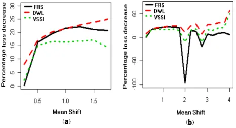
to 17.36%, 19.76% and 14.08% respectively. The results are plotted in

Figure 1. This ﬁgure shows that for small to moderate shifts (Figure

1 (a)), the V SSC scheme has a greater economic advantage versus the

DW L, V SSI and F RS schemes. This is not unexpected. Faraz et al

(2010b) concluded that theT2−DW Lcontrol chart is more economical

than theT2−V SSI,T2−V SS,T2−V SI and T2−F RS charts. So,

we can conclude that, specially for small to moderate shifts, theV SSC

scheme is more economical than otherV RS and F RS schemes.

(14)

5 Sensitivity Analysis

In this section, we conduct a sensitivity analysis for the above example to study the eﬀects of the model parameters (process parameters and

cost parameters) on the economic design of theT2−V SSC chart. This

study is carried out using experimental design and linear regression anal-ysis. In each linear regression model, given values of process parameters (p, λ, d, T0, T1, m) and given values of cost parameters (V0, V1, C0, C1, s)

are regarded as possible independent variables while the test parameters and the expected total cost are treated as the dependent variables. The eleven model parameters considered in the sensitivity analysis and their corresponding level plans are shown in Table 1. In our plan we have nine parameters with two levels and two parameters with four levels.

To study the eﬀect of the model parameters on the solution of

eco-nomic design of the V SSC scheme based on the data in Table 6, the

statistical software SPSS is used to run the regression analysis for each dependent variable. For each dependent variable, the output of SPSS includes an ANOVA table for regression and a table of regression co-eﬃcients, showing the corresponding information about statistical hy-pothesis testing. Table 7 is the SPSS output for the small sample size

(n1). From the ANOVA in Table 7(a), we conclude that at least one

model parameter signiﬁcantly aﬀects the value of small sample size. On

examining Table 7(b), we ﬁnd that both the parameters dand C1

sig-niﬁcantly aﬀect the value of sample size n1. We note that the sign of

the coeﬃcient ofdandC1 is negative which indicates that higher values

of the magnitude of the shift and the expected cost of searching for an

assignable cause reduce the sample sizen1. Table 8 is based on the large

sample size (n2) and shows that the parametersd and V0 signiﬁcantly

aﬀect the value of sample sizen2. Increasing values of the magnitude of

the shift cause a decrease in the sample size n2 and lower values of the

average proﬁt per hour earned when the process is in control leads to larger values forn2.

Tables 9 and 10 are the SPSS outputs for the warning lines (w1,

w2). From these tables, we see that the only model parameter that

signiﬁcantly aﬀects the warning lines is p. Higher values of the number

of correlated quality characteristics leads to larger values forw1 andw2.

Tables 11 and 12 which display the results for changing control limits

(k1, k2), show that both parameters d and p signiﬁcantly aﬀect the

control limits. Higher values of the magnitude of the shift and number

of correlated quality characteristics lead to larger values for k1 and k2.

Table 13 gives the SPSS output for the expected loss value E(L). It is

(15)

obvious that the parameters λ, V0, T1,d and m signiﬁcantly aﬀect the

expected loss. Since a higher penalty cost of defective products leads to a higher total cost, to reduce the total cost, the penalty cost of defective products should be decreased as much as possible.

6 Conclusion

In the present paper, the economic design of the T2 −V SSC chart

is developed based on the cost model proposed by Costa and Rahim (2001). The expected total cost per hour is minimized using GA and

ﬁnally, the T2 −V SSC chart and the T2 −DW L, T2 −V SSI and

T2 ₋_{F RS} _{control charts are compared from an economic viewpoint.}

Also, sensitivity analysis is carried out to investigate the eﬀects of model parameters on the solution of the economic design. The results indicate that among the four possible schemes, the expected hourly loss of the

V SSC scheme is smaller than the DW L, V SSI and F RS schemes, specially for small to moderate shifts. These results are presented on a

graph. Since Faraz et al (2010b) concluded that theT2−DW Lcontrol

chart is more economical when compared with T2−V SSI, T2−V SS,

T2−V SI and T2 −F RS control charts, we conclude that the V SSC

scheme is more economical than the otherV RS and F RS schemes.

Sensitivity analysis shows that C1, s, V1 and T0 have no signiﬁcant

impact on the optimal solution of the V SSC scheme, while the eight

parametersm,s,d,C0,V0,T1,λandpplay signiﬁcant role in inﬂuencing

the response parameters.

Acknowledgment

The authors are grateful to Professor Mahbanoo Tata for making many helpful comments and suggestions.

(16)

Tables

Table 1. Levels for each model parameter

Model parameter Level 1 Level 2 Level 3 Level 4

m 10 50 100 1000

d 0.5 1.0 1.5 2.0

s 5 10

C0 250 500

C1 50 500

V0 250 500

V1 50 100

T0 2.5 5

T1 1 10

λ 0.01 0.05

p 2 5

Table 2. Experimental layout of theL16(2942) array

No. m d s C0 C1 V0 V1 T0 T1 λ p

1 10 0.5 5 250 50 250 50 2.5 1 0.01 2

2 10 1.0 5 250 50 500 100 5 10 0.05 5

3 50 0.5 5 500 500 250 50 5 10 0.05 5

4 50 1.0 5 500 500 500 100 2.5 1 0.01 2

5 50 1.5 10 250 50 250 100 2.5 1 0.05 5

6 50 2.0 10 250 50 500 50 5 10 0.01 2

7 10 1.5 10 500 500 250 100 5 10 0.01 2

8 10 2.0 10 500 500 500 50 2.5 1 0.05 5

9 100 0.5 10 250 500 500 100 2.5 10 0.01 5

10 100 1.0 10 250 500 250 50 5 1 0.05 2

11 1000 0.5 10 500 50 500 100 5 1 0.05 2

12 1000 1.0 10 500 50 250 50 2.5 10 0.01 5

13 1000 1.5 5 250 500 500 50 2.5 10 0.05 2

14 1000 2.0 5 250 500 250 100 5 1 0.01 5

15 100 1.5 5 500 50 500 50 5 1 0.01 5

16 100 2.0 5 500 50 250 100 2.5 10 0.05 2

(17)

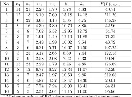
Table 3. Optimal set of parameters for ED of the T2₋ V SSCcontrol chart for 16 trails

No. n1 n2 w1 w2 k1 k2 E(L)V SSC

1 14 21 2.20 1.70 5.73 4.63 40.71

2 12 18 8.10 7.60 15.18 14.18 211.20

3 6 22 3.63 3.13 5.05 4.75 146.28

4 9 16 4.30 3.80 10.70 8.85 42.96

5 4 8 7.02 6.52 12.95 12.72 54.74

6 3 5 1.91 1.40 12.10 11.85 71.32

7 4 7 2.49 1.99 10.02 9.54 43.72

8 3 6 6.21 5.71 16.67 16.50 107.25

9 3 25 3.17 2.68 8.30 7.44 122.18

10 5 9 2.58 2.08 7.22 6.33 90.80

11 15 23 2.29 1.79 5.46 4.85 176.69

12 8 12 6.77 6.27 12.34 11.07 52.29

13 4 7 2.47 1.97 10.53 9.85 212.08

14 4 6 4.87 4.37 18.47 18.30 20.01

15 7 12 7.74 7.24 18.90 18.41 34.31

16 2 5 2.54 2.04 11.15 11.00 95.96

∗_{Minimum values of E(L) for given and optimal parameters}

Table 4.Optimal set of parameters for ED ofT2₋_{V SSC}_and_T2₋_{F RS}

control charts

d n1 n2 w1 w2 k1 k2 E(L)V SSC k0 h0 n0 E(L)F RS % of improvement 0.25 2 5 1.07 0.57 1.88 1.60 58.34∗ 1.67 10 3 58.43 0.15 0.50 13 23 2.27 1.77 5.65 4.68 40.71∗ 5.21 5.96 16 48.71 16.42 0.75 10 17 2.63 2.13 7.51 6.41 31.02∗ 7.09 4.49 12 38.55 19.53 1.00 7 12 3.57 3.07 8.72 7.38 25.06∗ 8.36 3.65 8 31.98 21.64 1.25 5 10 3.61 3.11 9.51 8.66 21.43∗ 9.32 3.08 8 27.48 22.02 1.50 4 7 2.59 2.09 10.36 9.64 19.14∗ 10.10 2.68 5 24.23 21.01 1.75 3 5 1.89 1.39 11.16 10.37 17.25∗ 10.75 3.37 4 21.76 20.73 2.00 2 4 1.96 1.45 11.40 3.60 39.23 11.31 2.13 3 19.83∗ -97.83 2.25 2 4 1.97 1.46 11.90 10.73 15.66∗ 11.80 1.94 3 18.27 14.29 2.50 2 4 1.97 1.47 12.30 11.34 14.83∗ 12.23 1.78 3 16.98 12.66 2.75 2 59 15.96 4.60 19.39 5.10 19.12 12.83 1.76 3 15.93∗ -20.03 3.00 2 6 3.18 2.65 14.82 11.80 14.10∗ 13.54 1.80 3 15.18 7.11 3.25 2 20 6.62 5.26 15.26 10.20 14.09∗ 14.29 1.83 3 14.65 3.82 3.50 2 4 1.97 1.47 18.40 13.76 13.09∗ 15.08 1.85 3 14.29 8.40 3.75 2 4 1.97 1.46 18.75 14.89 12.75∗ 19.92 1.88 3 14.03 9.12 4.00 2 56 17.95 10.50 17.97 11.00 13.07∗ 16.81 1.88 3 13.87 5.77

∗_{Minimum values of E(L) for given and optimal parameters}

Table 5. Optimal set of parameters for ED of theT2₋_{DW L}_{control chart}

d n1 n2 h1 h2 wN wT k E(L)DW L E(L)V SSC % of improvement

0.25 2 4 10.00 9.00 1.05 1.55 1.67 63.39 58.34∗ 7.97 0.50 13 20 6.09 5.70 1.95 2.45 5.21 49.17 40.71∗ 17.21 0.75 11 18 4.59 3.79 4.45 4.95 7.09 38.85 31.02∗ 20.15 1.00 7 14 3.75 2.86 4.57 5.07 8.36 31.89 25.06∗ 21.42 1.25 5 15 3.18 0.19 5.40 5.90 9.31 27.74 21.43∗ 22.75 1.50 4 9 2.10 2.78 3.67 4.17 10.10 25.11 19.14∗ 23.77 1.75 3 16 2.47 0.89 5.92 6.42 10.76 23.01 17.25∗ 25.03 2.00 2 8 2.23 1.43 3.99 4.49 5.21 43.69 39.23∗ 10.21 2.25 2 16 2.04 0.33 5.96 6.46 11.31 20.73 15.66∗ 24.46 2.50 2 11 1.88 0.72 4.83 5.33 11.83 20.68 14.83∗ 28.29 2.75 2 4 1.88 1.50 1.89 2.39 12.87 20.59 19.12∗ 7.14 3.00 2 13 1.90 0.51 5.31 5.81 13.62 19.40 14.10∗ 27.32 3.25 2 5 1.93 1.49 2.57 3.07 14.26 19.31 14.09∗ 27.03 3.50 2 6 1.95 1.39 3.14 3.64 15.20 19.03 13.09∗ 31.21 3.75 2 12 1.98 0.71 5.10 5.60 16.22 18.58 12.75∗ 31.38 4.00 2 7 1.98 1.30 3.56 4.06 7.03 30.46 13.07∗ 57.09 ∗_{Minimum values of E(L) for given and optimal parameters}

(18)

Table 6. Optimal set of parameters for ED of theT2₋_{V SSI}_{control chart}

d n1 n2 h1 h2 w k E(L)V SSI E(L)V SSC % of improvement

0.25 2 4 10.00 9.00 0.50 1.67 59.55 58.34∗ 2.03 0.50 11 18 7.60 4.01 1.30 5.21 48.02 40.71∗ 15.22 0.75 8 13 6.57 2.06 1.30 7.09 37.19 31.02∗ 16.59 1.00 4 9 5.80 0.87 1.18 8.36 29.99 25.06∗ 16.44 1.25 2 7 4.65 1.06 1.19 9.31 25.75 21.43∗ 16.78 1.50 2 6 4.07 1.01 1.25 10.10 23.07 19.14∗ 17.03 1.75 2 5 3.96 0.14 1.09 10.76 20.17 17.25∗ 14.48 2.00 2 19 5.03 1.39 3.34 5.21 35.44∗ 39.23 -10.69 2.25 1 4 2.66 1.13 1.30 11.31 18.23 15.66∗ 14.10 2.50 1 4 2.40 1.07 1.29 11.83 17.85 14.83∗ 16.92 2.75 2 5 1.97 1.60 1.72 12.87 17.32∗ 19.12 -10.39 3.00 2 5 2.06 1.60 1.70 13.63 16.87 14.10∗ 16.42 3.25 2 5 2.00 1.70 1.75 14.26 16.54 14.09∗ 14.81 3.50 2 5 2.05 1.70 1.73 15.20 16.30 13.09∗ 19.69 3.75 2 5 2.11 1.70 1.72 16.22 16.13 12.75∗ 20.95 4.00 2 17 3.14 1.65 3.90 7.03 26.61 13.07∗ 50.88

∗ _{Minimum values of E(L) for given and optimal parameters}

Figure 1: Percentage loss decrease of E(L) for the VSSC scheme versus FRS, DWL and VSSI schemes as a function of d.

Table 7(a). ANOVA table for sample sizen1

Source Sum of Squares DF Mean Square F Value P−V alue

Regression∗ 153.675 2 76.837 10.166 0.002 Residual 98.262 13 7.559

Total 251.937 15

∗ _{Predictors: (Constant),}_d_,_C₁

Table 7(b). Coeﬃcients table for sample size n1

Model βˆ Std. Error t P−V alue

Constant 14.313 1.882 7.607 0.000

d -4.650 1.230 -3.782 0.002

C1 -0.008 0.003 -2.455 0.029

(19)

Table 8(a). ANOVA table for sample sizen2

Total 761.750 15

∗ _{Predictors: (Constant),}_d_,_V₀

Table 8(b). Coeﬃcients table for sample size n2

Constant 22.750 2.427 9.373 0.000

d -11.400 1.121 -10.168 0.000

V0 0.011 0.005 2.194 0.047

Table 9(a). ANOVA table for warning linew1

Total 72.299 15

∗ _{Predictors: (Constant),}_p

Table 9(b). Coeﬃcients table for warning linew1

Constant 0.370 0.899 0.415 0.685

p 1.114 0.234 4.756 0.000

Table 10(a). ANOVA table for warning linew2

Total 72.324 15

∗ _{Predictors: (Constant),}_p

Table 10(b). Coeﬃcients for warning linew2

Constant -0.113 0.891 -0.149 0.884

p 1.115 0.234 4.763 0.000

Table 11(a). ANOVA table for control limitk1

Total 289.957 15

∗ _{Predictors: (Constant),}_d_,_p

(20)

Table 11(b). Coeﬃcients table for control limitk1

Constant -0.581 1.912 -0.304 0.766

d 5.425 1.01 5.367 0.0020

p 1.456 0.377 3.865 0.002

Table 12(a). ANOVA table for control limitk2

Total 309.421 15

∗ _{Predictors: (Constant),}_d_,_p

Table 12(b). Coeﬃcients table for control limitk2

Constant -2.024 1.718 -1.178 0.260

d 5.892 0.909 6.485 0.000

p 1.511 0.339 4.463 0.001

Table 13(a). ANOVA table forE(L)

Total 59017.781 15

∗ _{Predictors: (Constant),}_λ_,_V

0,T1,d,m Table 13(b). Coeﬃcients table forE(L)

Constant -47.055 19.397 -2.426 0.036

λ 2085.937 221.095 9.435 0.000

V0 0.217 0.035 6.127 0.000

T1 5.383 0.983 5.478 0.000

d -31.318 7.910 -3.959 0.003

m 0.027 0.011 2.532 0.030

References

Aparisi, F. (1996), Hotelling’s T2 control chart with adaptive

sam-ple sizes. International Journal of Production Research,34 (10),

2853-2862.

(21)

Aparisi, F. and Haro, C. L. (2001), Hotellings T2 control chart with variable sampling intervals. International Journal of Production

Research,39(14), 3127-3140.

Aparisi, F. and Haro, C. L. (2003), A comparison of T2 control charts

with variable sampling scheme as opposed to MEWMA chart.

In-ternational Journal of Production Research,41, 2169-2182.

Burr, I. W. (1969), Control charts for measurements with varying

sam-ple sizes. Journal of Quality Technology,1, 163-167.

Chen, Y. K. (2006a), Economic design of variable sampling intervals

T2 control charts- A hybrid Markov Chain approach with genetic

algorithms. Expert System with Applications,33, 683-689.

Chen, Y. K. (2006b), Economic design of T2 control charts with the

V SSIsampling scheme. Quality & Quantity, DOI:10.1007/s11135-007-9101-7.

Chen, Y. K. and Hsieh, K. L. (2007), Hotelling’sT2 control chart with

variable sample size and control limit. European Journal of

Oper-ational Research,182, 1251-1262, DOI:10.1016/j.ejor.2006.09.046.

Chou, C. Y., Chen, C. H., and Chen, C. H. (2006), Economic design

of variable sampling intervalsT2 control charts using genetic

algo-rithms. Expert System with Applications, 30, 233-242.

Cinlar, E. (1975), Introduction to Stochastic Process. Prentice Hall, Englewood Cliﬀs, NJ.

Costa, A. F. B. (1994), ¯X chart with variable sample sizes. Journal of

Quality Technology,21, 155-163.

Costa, A. F. B. (1997), ¯Xchart with variable sample sizes and sampling

intervals. Journal of Quality Technology,29(2), 197-204.

Costa, A. F. B. and Rahim, M. A. (2001), Economic design of ¯Xcharts

with variable parameters: the Markov Chain approach. Journal of

Applied Statistics,28(7), 875-885.

Duncan, A. J. (1956), The Economic Design of ¯Xcharts used to

Main-tain Current Control of a Process. Journal of American Statistical

association, 51(274), 228-242.

(22)

Daudin, J. J. (1992), Double sampling ¯X charts. Journal of Quality

Technology,24, 78-87.

Faraz, A. and Moghadam, M. B. (2008), Hotelling’s T2 control chart

with two adaptive sample sizes. Quality & Quantity, International

Journal of Methodology, 43(6), 903-912.

Faraz, A. and Parsian, A. (2006), Hotelling’s T2 control chart with

double warning lines. Journal of Statistical Papers, 47, 569-593.

Faraz, A., Chalaki, K., and Moghadam, M. B. (2009a), On the

prop-erties of the Hotelling’s T2 control chart with variable sampling

intervals. Quality & Quantity, International Journal of Methodol-ogy, DOI:10.1007/s11135-010-9314-z.

Faraz, A., Kazemzade, R. B., and Saniga E. (2009b), Economic and

economic-statistical design of T2 control chart with two adaptive

sample sizes. Journal of Statistical Computation and Simulation, DOI:10.1080/00949650903062574.

Faraz, A., Kazemzade, R. B., and Moghadam, M. B. (2010a), A study

on the economic propertis of the T2 control chart with adaptive

sample sizes. Technometrics, (Accepted to appear 2010).

Faraz, A., Kazemzade, R. B., Moghadam, M. B., and Parsian, A. (2010b), On the Advantages of Economically Design Variable

Sam-ple Sizes and Sampling IntervalsT2 Control Chart- Double

Warn-ing Line Scheme. Quality & Quantity, Interational Journal of

Methodology, (Accepted to appear 2010).

Goldberg, D. E. (1989), Genetic algorithms in search, optimization, and machine learning reading. Addison-Wesley, MA.

Hotelling, H. (1947), Multivariate quality control illustrated by the air testing of sample bombsights, in Techniques of Statistical Analysis, C. Eisenhart, M.W. Hastay, and W.A. Wallis, eds., MacGraw-Hill, NewYork, 111-184.

Lorenzen, T. J. and Vance, L. C. (1986), The Economic Design of

Control Charts: A Uniﬁed Approach. Technometrics,28(1), 3-10.

Mason, R. L. and Young J. C. (2002), Multivariate statistical process control with industrial applications. Society for Industrial

Mathe-matics, Arabian Journal for Science and Engineering,36(7),

1461-1470.

(23)

Montgomery, D. C. and Klatt, P. J. (1972), Economic Design of T2

Control Charts to maintain current control of a process.

Manage-ment Science,19(1), 76-89.

Prabhu, S. S., Montgomery, D. C., and Runger, G. C. (1994), A

combined adaptive sample sizes and sampling interval ¯X control

scheme. Journal of Quality Technology,26(3), 164-176.

Prabhu, S. S., Runger, G. C., and Keats, J. B. (1993), ¯X chart with

adaptive sample sizes. International Journal of Production

Re-search,31(12), 2895-2909.

Reynolds Jr, M. R. (1988), Optimal variable sampling interval control

charts. Sequential Analysis,8, 361-379.

Reynolds Jr, M. R. and Arnold, J. C. (1989), Optimal one-side She-whart control chart with variable sampling ntervals. Sequential

Analysis,9, 51-77.

Runger, G. C. and Pignatiellow, J. J. (1991), Adaptive sampling for

process control. Journal of Quality Technology, 23(2), 133-155.

Zimmer, L. S., Mongomery, D. C., and Runger, G. C. (1998),

Evalua-tion of a three-state adaptive sample size ¯X control chart.

Inter-national Journal of Production Research,36(3), 733-743.

(24)