ORIGINAL ARTICLE
Co-integration between globalisation and economic growth
Cândida Ferreira
ISEG, Universidade de Lisboa and UECE
Abstract: This paper analyses the co-integration relationship between globalisation and economic growth of 26 more or less developed countries across almost all Continents for the time period 1970–2013. Globalisation is proxied by the overall globalisation index and the sub-indices representing economic globalisation, social globalisation and political globalisation, all provided by the Swiss Economic Institute. Economic growth is measured through the natural logarithm of the real Gross Domestic Product, sourced from the World Development Indicators which are provided by the World Bank. Co-integration is tested with quantile co-integration regressions. The results obtained clearly confirm the existence of non-linear co-integration relationships between the considered globalisation indices and the real economic growth.
Keywords: Economic growth; globalisation; KOF globalisation indices; co-integration; quantile regressions
1. Introduction
Globalisation has often been considered as a key factor for economic growth as at least from an economic and policy perspective, the relationship between globalisation and economic growth is undoubtedly relevant.
There is also a general agreement concerning the belief that globalisation has been making people and countries more interdependent and that this interdependence is not strictly economic, but also political and social. Therefore, the definition of relevant measures of globalisation is not easy to formulate as a reliable indicator should consider economic, political and social aspects.
These multiple dimensions of globalisation were constructively taken into account by Dreher[5], updated and
discussed in Dreher et al.[6,7] , who created an overall index of globalisation covering economic integration, social
integration and political integration. These authors critically analyse the differences between the existing globalisation indices, clearly underlying their inherent limitations, but also defending the relevance of these indices as promising means for providing objectives data to measure globalisation meaningfully, despite the different methodologies, choices of variables and weights.
Nowadays, the index presented in Dreher[5]and Dreher et al.[6,7]is known as the KOF index of globalisation and is
provided by the Swiss Economic Institute.
Since its construction, the KOF globalisation index and its main sub-indices have been used in many empirical analyses. Among others, Chang and Lee[1]use panel data including 23 countries within the Organisation for Economic
Co-operation and Development (OECD) for the period 1970–2006 and apply panel co-integration techniques to test the main dimensions: economic, political and social integration. The main conclusions point to the existence of long-term
Copyright © 2017 Cândida Ferreira doi: 10.18686/fm.v2i2.917
This is an open-access article distributed under the terms of the Creative Commons Attribution Unported License
(http://creativecommons.org/licenses/by-nc/4.0/), which permits unrestricted use, distribution, and reproduction in any medium, provided the original work is properly cited.
long-term co-movements and causality between economic growth and the overall KOF globalisation index and its three unidirectional causality running from the overall index of globalisation, economic globalisation and social globalisation to economic growth.
Changet al.[2]also test the relationship between growth in gross domestic product (GDP) and the KOF globalisation index
and its three main dimensions using panel co-integration techniques, considering the G7 countries in the period 1970–2006. They conclude that both the overall globalisation index and the social globalisation index have a direct positive impact on GDP growth.
The same variables are used in panel co-integration estimations by Ying et al.[16]to test the long-term
relationships between economic growth and globalisation in the Association of Southern Asian Nations (ASEAN) over the period 1970–2008, concluding that economic globalisation has a significantly positive influence on economic growth, but social globalisation has a negative influence on economic growth and political globalization has a non-significant negative effect.
Chang et al.[3]test the existence of non-linear relationships between real output and the KOF globalisation index
and its three main dimensions (economical, political and social) through quantile co-integration regressions and considering the G7 countries over the period 1970–2006. They conclude overall that the three dimensions of globalisation act as engines of real output and play a key role in long-term growth.
Kazar and Kazar[10]use the KOF globalisation index to investigate the relationship between globalisation, financial
development and economic growth, with panel co-integration techniques, in OECD and non-OECD countries classified according to their income levels from 1980 to 2010 and obtain different conclusions according to the country classification. More precisely, they conclude that the driving force of economic growth in terms of globalisation for low-income and non-OECD high-income countries is mainly the social globalisation dimension; for high-income OECD and upper middle-income economies, it is the political globalisation dimension; for lower middle-income countries, it is the economic globalisation dimension.
In spite of the vast literature on globalisation issues and the recognition of their relevance not only for the academic and scientific community, but also for policymakers and the general public, the relationship between the different aspects of globalisation and economic growth is still unresolved and controversial, thus deserving further examination.
Is this paper we contribute to the literature by testing the existence of co-integration between economic growth and the KOF Overall Globalisation Index as well as the 3 KOF sub-indices of globalisation, representing the economic, social and political dimensions of globalisation .
We consider 26 countries with different levels of development across almost all continents. The period of analysis covers the period 1970–2013. In our estimations we test the long-term equilibrium relationships applying quantile co-integration regressions.
The remainder of this paper is organised as follows: Section 2 describes the methodology and the data used; Section 3 presents the results obtained and Section 4 concludes.
2. Methodology and data
The application of co-integration techniques provides an appropriate conceptual framework to analyse the long-term relationship between economic growth and globalisation. The existence of co-integration implies that causality exists between the two series, although it does not indicate the direction of the causal relationship. The general definition of co-integration follows that of Engle and Granger[8], meaning that two non-stationary series, xt and yt, with
a stationary linear combination of these series, zt, which can be defined using the equation:
zt = xt - a - byt (1)
where a and b are constant terms.
Thus, we should first test the stationarity of the series. Here we use the augmented Dickey–Fuller (ADF; Dickey and Fuller[4]) and the Phillips–Perron (PP; Phillips and Perron[13]) unit root tests.
Then, we will follow Xiao[15]in testing the presence of co-integration using quantile regressions, which allow us to
analyse the co-integration relationships between the variables considered across several quantiles, taking into account the possibility that the co-integration vectors might not be constant. In the next sub-sections we provide brief descriptions of these methodological steps.
2.1 Unit root tests
A series possessing a unit root is a non-stationary series. However, as has been clearly demonstrated, for instance by Granger and Swanson[9], the first difference of this series can be stationary.
Beginning with the definition of a first-order autoregressive process, AR(1), we estimate:
yt = yt-1 + t (2)
where t is the zero mean, independent and identically distributed (i.i.d.), with variance
2 .From the previous equation, we can obtain:
yt - yt-1 =t = t (3)
wheret is the zero mean, i.i.d., with variance
2. Thust can be a stationary series, even if yt is non-stationary.The null hypothesis of the ADF unit root test is that the series has a unit root. From the AR(1) process represented in equation (2), we can obtain:
yt =+yt-1 + t + t (4)
whereis the constant term,is a coefficient,t is the time trend and t is also a zero mean, i.i.d., with variance
2.Extending equation (4) with the inclusion of p lagged differences and removing the eventual serial correlation in the lagged variables, we obtain the ADF equation:
yt =+yt-1 +t +1yt-1 +2yt-2 + … +pyt-p + t (5)
The number of augmenting lags (p) should be determined by minimizing the Schwartz Bayesian information criterion (SBIC; Schwartz[14]), or minimizing the Akaike information criterion (AIC), or dropping lags until the last lag
is statistically significant.
The PP test statistics can be viewed as Dickey–Fuller statistics that have been made robust to serial correlation. The advantages of the PP unit root test over the ADF test are that the PP test is robust to general forms of heteroscedasticity in the error term ut and that it is not necessary to specify a lag length for the test regression. The test regression for the PP unit root test is given by:
yt =+yt-1 + ut (6)
2.2 Quantile co-integration regressions
Traditional co-integration tests are mostly based on the assumption of constant co-integrating vectors and this may be one of the reasons why in many cases co-integration has not been found among series that are seemingly co-integrated (as well underlined, among others, by Park and Hahn[12]).
In terms of the long-term relationship between globalisation and real output growth, we may consider that it is primarily a time-varying long-term process and should not be considered as constant over time. Thus, instead of focusing on the average relationship between globalisation and economic growth through a conditional mean function, we may assume that these long-term relationships are non-linear and can be influenced by time-varying shocks.
Under these assumptions, quantile co-integration methodology is considered more adequate than traditional co-integration testing. Xiao[15] analyses the evolution of the quantile regression approach, namely in financial
applications related to risk management, portfolio optimisation and asset pricing, demonstrating that this approach can capture the influences of conditional variables on the location, scale and shape of the conditional distribution of the response and thus represent a significant extension of the classical co-integration models.
Therefore, quantile methodology provides the possibility of quantifying the impact of the signs and magnitudes of a shock on the long-term vector and the different values of the co-integrating coefficients, which represent positive or negative shocks, can be detected. Moreover, quantile regressions allow for additional volatility in the dependent variables, in addition to the regressors, and provide an interesting class of the co-integration model with conditional heteroscedasticity; the estimated co-integration coefficients may also be influenced by the innovations in each period and thus will vary from quantile to quantile.
Following Xiao[15] and the simplifications presented in Lee and Zeng[11] and Chang et al.[3], we recall that the
traditional co-integration model can be represented with the general equation yt =+ ’xt + ut, where yt and xt are integrated at order 1 and ut is stationary in level. To address the endogeneity that may occur in traditional co-integration models, it is possible to decompose ut into lead-lag terms and the pure innovation component, t, obtaining the following model:
' t
K
K
j t j j
t
t x x
y
(7)
Considering the -th quantile of t with Q ( ), which is conditional ont (and assuming thatt = xt , xt-i ,
j), the -th quantile of yt can be written as:
) ( )'
( )
( 1
x
x FQ K
K
j t j j
t t
yt
(8) where F(.) is the conditional distribution function of t.
Taking Zt to represent the vector of regressors consisting of zt = (1, xt) and (x’t-j, j = -K, …, K), = (,’t,
’-K, … ,’K)’ and() = ((),()’,’-K, … ,’K)’, where() = F -1(), we may re-write yt as:
yt =’ Zt +t (9)
and also:
)'
(
)
(
t ty
Z
Q
t
(10)Moreover, if we consider that t = t - F -1, we obtain Q t( ) = 0.
Therefore – and still following Xiao[15]– we can conclude that with this methodology the value of the co-integration
coefficients will be affected by the innovations in each time period and thus the co-integration vector will vary over the quantiles and will be quantile -dependent.
2.3 Data
We test the relationship between globalisation and the economic growth of 26 countries, spread across almost all continents, for the years 1970–2013: Australia, Austria, Brazil, Canada, Denmark, France, Germany, Greece, Iceland, India, Indonesia, Ireland, Italy, Japan, Mexico, the Netherlands, New Zealand (only from 1977), Norway, Portugal, South Africa, Spain, Sweden, Switzerland (only from 1980), Turkey, the United Kingdom (UK) and the United States of America (USA).
In this paper economic growth is represented by the natural logarithm of real GDP with data sourced from the World Development Indicators provided by the World Bank (series “GDP at market prices, constant 2010 US$”). Globalisation is proxied by the KOF indices provided by the Swiss database, here we include not only the overall index but also the three sub-indices measuring the three relevant dimensions of globalisation: economic, social and political.
3. Results
Following the methodological steps presented in the previous section we will first report the results obtained the two unit root tests and then present and discuss the results obtained with the quantile co-integration regressions.
3.1 ADF and PP unit root tests
In the first step we examine the stationarity of the series, implementing two unit root tests: ADF and PP. Before performing these tests, we selected the number of lags to be used in each situation. Using Stata software, we followed the results obtained with the most used criteria: the AIC and the SBIC.
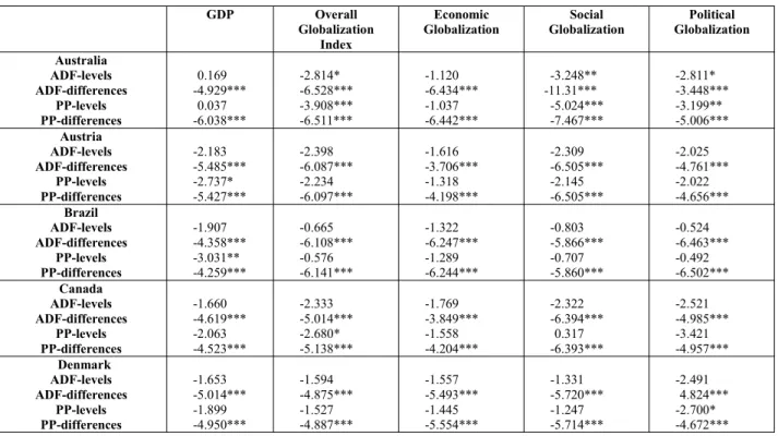
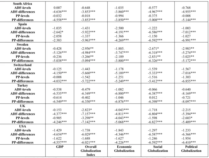
Table 1 presents the obtained ADF and PP unit root test results for the considered series, both in levels and in first differences. Almost all variables are non-stationary at their levels and become stationary at their first differences, showing that these variables are integrated in the order of I(1).
Table 1 – Test statistic values obtained with ADF and PP unit root tests
GDP Overall Globalization
Index
Economic
Globalization GlobalizationSocial GlobalizationPolitical Australia
ADF-levels ADF-differences
PP-levels PP-differences
0.169 -4.929***
0.037 -6.038***
-2.814* -6.528*** -3.908*** -6.511***
-1.120 -6.434*** -1.037 -6.442***
-3.248** -11.31*** -5.024*** -7.467***
-2.811* -3.448*** -3.199** -5.006***
Austria ADF-levels ADF-differences
PP-levels PP-differences
-2.183 -5.485*** -2.737* -5.427***
-2.398 -6.087*** -2.234 -6.097***
-1.616 -3.706*** -1.318 -4.198***
-2.309 -6.505*** -2.145 -6.505***
-2.025 -4.761*** -2.022 -4.656***
Brazil ADF-levels ADF-differences
PP-levels PP-differences
-1.907 -4.358*** -3.031** -4.259***
-0.665 -6.108*** -0.576 -6.141***
-1.322 -6.247*** -1.289 -6.244***
-0.803 -5.866*** -0.707 -5.860***
-0.524 -6.463*** -0.492 -6.502***
Canada ADF-levels ADF-differences
PP-levels PP-differences
-1.660 -4.619*** -2.063 -4.523***
-2.333 -5.014*** -2.680* -5.138***
-1.769 -3.849*** -1.558 -4.204***
-2.322 -6.394***
0.317 -6.393***
-2.521 -4.985*** -3.421 -4.957***
Denmark ADF-levels ADF-differences
PP-levels PP-differences
-1.653 -5.014*** -1.899 -4.950***
-1.594 -4.875*** -1.527 -4.887***
-1.557 -5.493*** -1.445 -5.554***
-1.331 -5.720*** -1.247 -5.714***
-2.491 4.824*** -2.700* -4.672***
France ADF-levels ADF-differences PP-levels PP-differences -3.841*** -4.439*** -3.555 -4.329*** -1.648 -5.226*** -1.542 -5.261*** -1.418 -5.466*** -1.375 -5.523*** -1.394 -6.843*** -1.269 -6.885*** -2.560 -4.628*** -2.263 -4.584*** Germany ADF-levels ADF-differences PP-levels PP-differences -1.791 -5.267*** -2.436 -5.155*** -1.342 -6.184*** -1.781 -6.187*** -1.379 -4.851*** -1.291 -4.902*** -0.729 -8.023*** -3.989*** -8.008*** -0.536 -5.453*** -0.585 -5.407*** Greece ADF-levels ADF-differences PP-levels PP-differences -1.439 -3.508*** -2.425 -3.470*** -0.564 -5.573*** -0.460 -5.586*** -0.947 -5.829*** -0.880 -5.806*** -0.265 -5.686*** -0.148 -5.734*** -1.247 -5.615*** -1.148 -5.561*** Iceland ADF-levels ADF-differences PP-levels PP-differences -1.482 -4.532*** -2.383 -4.521*** -1.577 -5.672*** -1.454 -5.789*** -0.699 -5.824*** -0.824 -5.806*** -1.488 -5.725*** -1.434 -5.759*** -2.488 -5.472*** -2.353 -5.437*** India ADF-levels ADF-differences PP-levels PP-differences 3.299 -5.948*** 4.201 -5.957*** 0.307 -5.699*** 0.437 -5.760*** -0.174 -5.643*** 0.792 -5.843*** -0.428 -4.711*** -0.233 -4.711*** -0.766 -8.491*** -0.855 -8.877*** Indonesia ADF-levels ADF-differences PP-levels PP-differences -1.564 -4.530*** -1.837 -4.513*** -0.888 -5.515*** -0.807 -5.531*** -0.919 -3.533*** -0.783 -5.158*** -0.217 -5.850*** -0.116 -5.843*** -2.216 -5.662*** -2.102 -5.678*** Ireland ADF-levels ADF-differences PP-levels PP-differences -0.702 -3.084** -0.740 -3.091** -1.082 -5.810*** -1.017 -5.783*** -2.192 -6.350*** -1.988 -6.392*** -0.296 -6.902*** -0.261 -7.056*** -1.303 -4.078*** -1.639 -4.076*** Italy ADF-levels ADF-differences PP-levels PP-differences -3.834*** -4.446*** -4.160*** -4.497*** -0.908 -5.207*** -0.811 -5.224*** -1.081 -4.968*** -0.487 -5.042*** -0.703 -6.487*** -0.650 -6.490*** -1.133 -4.654*** -1.343 -4.578*** Japan ADF-levels ADF-differences PP-levels PP-differences -3.467*** -4.188*** -4.449*** -4.154*** -0.115 -7.411*** -0.667 -7.718*** -0.865 -5.503*** -0.863 -5.439*** 0.340 -7.616*** -0.601 -7.663*** -0.655 -7.142*** -1.195 -7.557*** Mexico ADF-levels ADF-differences PP-levels PP-differences -2.267 -4.711*** -2.438 -4.676*** -0.717 -7.063*** -0.656 -7.114*** -0.518 -7.172*** -0.359 -7.285*** -0.706 -6.387*** -0.683 -6.394*** -2.001 -5.575*** -2.170 -5.548*** Netherlands ADF-levels ADF-differences PP-levels PP-differences -1.289 -3.697*** -1.685 -3.617*** -2.719* -5.481*** -2.877** -5.537*** -2.276 -5.481*** -2.790* -5.480*** -2.201 -6.801*** -2.415 -6.815*** -2.052 -3.832*** -2.377 -4.786*** New Zealand ADF-levels ADF-differences PP-levels PP-differences 0.137 -3.748*** -0.028 -3.803*** -0.999 -3.128** -0.972 -3.120** -1.771 -4.478*** -1.620 -4.532*** -0.886 -3.536*** -0.999 -3.555*** -0.449 -3.493*** -0.710 -3.476*** Norway ADF-levels ADF-differences PP-levels PP-differences -2.526 -3.055** -3.612*** -2.999** -2.503 -6.217*** -2.186 -6.233*** -2.211 -7.498*** -2.347 -7.502*** -1.122 -6.586*** -1.135 -6.587*** -2.270 -4.585*** -2.415 -4.456*** Portugal ADF-levels ADF-differences PP-levels -2.235 -3.727*** -3.074** -0.535 -3.950*** -0.616 -0.970 -4.992*** -0.975 -0.025 -5.704*** -0.069 -1.236 -3.430*** -1.327
South Africa ADF-levels ADF-differences PP-levels PP-differences 0.007 -4.636*** -0.032 -4.558*** -0.648 -3.853*** -0.018 -3.853*** -1.035 -3.860*** -0.994 -3.850*** -0.577 -4.967*** -0.375 -5.008*** -0.768 -4.955*** -0.008 -5.144*** Spain ADF-levels ADF-differences PP-levels PP-differences -1.035 -2.642* -2.058 -2.383 -1.431 -5.922*** -1.337 -5.963*** -2.500 -4.191*** -1.366 -4.269*** -1.222 -6.586*** -1.150 -6.592*** -1.003 -7.012*** -1.027 -6.991*** Sweden ADF-levels ADF-differences PP-levels PP-differences -0.428 -5.126*** -0.236 -5.038*** -2.956** -4.984*** -3.266** -5.094*** -1.885. -3.747*** -2.189 -3.800*** -2.671* -6.318*** -2.831** -6.326*** -2.983** -5.274*** -3.025** -5.172*** Switzerland ADF-levels ADF-differences PP-levels PP-differences -0.125 -4.150*** -0.008 -4.032*** -1.443 -5.660*** -1.542 -5.722*** -1.178 -5.189*** -1.251 -5.249*** -1.539 -5.333*** -1.516 -5.412*** -1.567 -7.016*** -1.303 -6.855*** Turkey ADF-levels ADF-differences PP-levels PP-differences -0.538 -6.535*** -0.614 -6.549*** -0.479 -6.349*** -0.402 -6.350*** -1.082 -6.880*** -1.046 -6.876*** -0.066 -6.387*** 0.012 -6.398*** -0.640 -8.169*** -0.721 -8.097*** UK ADF-levels ADF-differences PP-levels PP-differences -0.153 -4.377*** -0.905 -4.246*** -2.823* -7.157*** -3.298** -7.142*** -4.043*** -4.811*** -4.043*** -5.068*** -1.718 -6.804*** -1.598 -6.827*** -2.215 -5.394*** -2.603* -5.409*** USA ADF-levels ADF-differences PP-levels PP-differences -1.429 -4.654*** -1.622 -4.557*** -1.738 -6.029*** -1.688 -6.021*** -1.843 -4.346*** -1.627 -4.226*** -1.297 -6.587*** -1.246 -6.592*** -1.233 -6.366*** -1.954 -6.410*** GDP Overall Globalization Index Economic
Globalization GlobalizationSocial GlobalizationPolitical
* Statistically significant at 10%; ** statistically significant at 5%; *** statistically significant at 1%.
Source: Author’s results obtained using STATA software.
3.2 Results obtained with quantile co-integration regressions
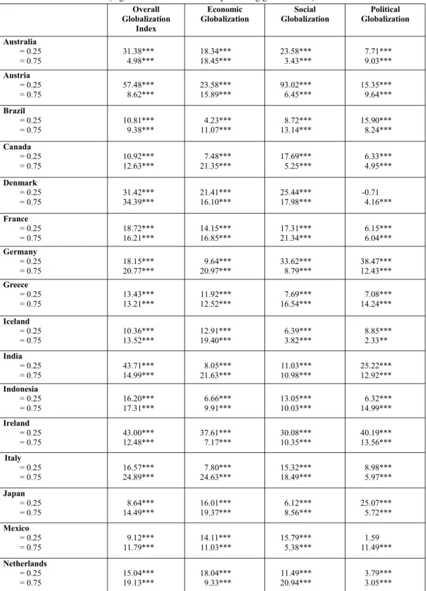
Following the methodology presented in the previous section, we estimate quantile co-integration regressions considering two quantiles: = 0.25 and = 0.75.
Table 2 reports the t-statistics for each of these regressions and in general terms demonstrates the statistical robustness of the results obtained, confirming the existence of non-linear co-integrating relationships between the countries’ economic growth and the globalisation indicators considered.
A detailed analysis of the results presented in Table 2 reveals that for 23 countries there are no doubts concerning the statistical robustness of the quantile regressions as in all situations they are statistically significant (and almost always at the 1% level).
With regard to the other countries, in general the results raise few doubts as the results are statistically significant for at least one of the considered quantiles.
The main doubts are related to the results obtained for the political globalisation for Denmark and Mexico (but only for the quantile = 0.25) and for Sweden (in this case for the quantile = 0.75)
These results may be explained mostly in terms of the particular definition of the globalisation indices considered, taking into account the relevant discussion, for example, in Dreher et al[7], and the arguments that the globalisation
variables and weights. Therefore, we should be very cautious in our conclusions regarding the results obtained for these three countries (Denmark, Mexico and Sweden) but. in general, these results may be interpreted as a confirmation of the non-linearity of the co-integration relationships between economic growth and globalisation.
Table 2 – Results (t-statistics) obtained with quantile co-integration regressions (log GDP and the variables representing globalization)
Overall Globalization
Index
Economic
Globalization GlobalizationSocial GlobalizationPolitical Australia
= 0.25
= 0.75 31.38***4.98*** 18.34***18.45*** 23.58***3.43*** 7.71***9.03***
Austria
= 0.25
= 0.75 57.48***8.62*** 23.58***15.89*** 93.02***6.45*** 15.35***9.64***
Brazil
= 0.25
= 0.75 10.81***9.38*** 11.07***4.23*** 13.14***8.72*** 15.90***8.24***
Canada
= 0.25
= 0.75 10.92***12.63*** 21.35***7.48*** 17.69***5.25*** 6.33***4.95***
Denmark
= 0.25
= 0.75 31.42***34.39*** 21.41***16.10*** 25.44***17.98*** -0.714.16***
France
= 0.25
= 0.75 18.72***16.21*** 14.15***16.85*** 17.31***21.34*** 6.15***6.04***
Germany
= 0.25
= 0.75 18.15***20.77*** 20.97***9.64*** 33.62***8.79*** 38.47***12.43***
Greece
= 0.25
= 0.75 13.43***13.21*** 12.52***11.92*** 16.54***7.69*** 14.24***7.08***
Iceland
= 0.25
= 0.75 10.36***13.52*** 12.91***19.40*** 6.39***3.82*** 8.85***2.33**
India
= 0.25
= 0.75 43.71***14.99*** 21.63***8.05*** 10.98***11.03*** 25.22***12.92***
Indonesia
= 0.25
= 0.75 16.20***17.31*** 6.66***9.91*** 13.05***10.03*** 14.99***6.32***
Ireland
= 0.25
= 0.75 43.00***12.48*** 37.61***7.17*** 30.08***10.35*** 40.19***13.56***
Italy
= 0.25
= 0.75 16.57***24.89*** 24.63***7.80*** 15.32***18.49*** 8.98***5.97***
Japan
= 0.25
= 0.75 14.49***8.64*** 16.01***19.37*** 6.12***8.56*** 25.07***5.72***
Mexico
= 0.25
= 0.75 11.79***9.12*** 14.11***11.03*** 15.79***5.38*** 11.49***1.59
Netherlands
= 0.25
New Zealand
= 0.25
= 0.75 12.96***17.33*** 15.54***17.69*** 10.79***9.72*** 10.18***6.59***
Norway
= 0.25
= 0.75 34.16***22.51*** 19.06***13.67*** 35.27***12.66*** 3.30***4.63***
Portugal
= 0.25
= 0.75 19.99***13.11*** 14.93***19.11*** 12.07***14.25*** 15.92***12.74***
South Africa
= 0.25
= 0.75 7.68***7.31*** 7.75***5.70*** 18.17***5.87*** 12.68***8.84***
Spain
= 0.25
= 0.75 16.65***15.64*** 20.31***13.21*** 22.68***8.75*** 23.71***7.86***
Sweden
= 0.25
= 0.75 23.33***7.51*** 22.93***14.68*** 36.53***3.84*** 3.58***0.99
Switzerland
= 0.25
= 0.75 7.68***4.13*** -1.74**2.20** 13.50***10.24*** 5.51***4.84***
Turkey
= 0.25
= 0.75 13.59***26.56*** 7.53***8.16*** 12.57***43.09*** 15.71***10.29***
UK
= 0.25
= 0.75 36.26***6.00*** 10.87***4.67*** 31.17***11.85*** -2.94***2.44**
USA
= 0.25
= 0.75 25.85***15.30*** 21.06***6.17*** 13.80***19.86*** 12.50***5.87***
Overall Globalization
Index
Economic
Globalization GlobalizationSocial GlobalizationPolitical
* Statistically significant at 10%; ** statistically significant at 5%; *** statistically significant at 1%. Source: Author’s results obtained using STATA software.
4. Concluding remarks
In this paper we confirm the non-linearity of the co-integrating long-term relationships between real GDP growth and globalisation in -26 countries across almost all continents, covering the period 1970–2013.
Globalisation is proxied by the KOF overall globalisation index as well as by the subindices representing economic, social and political globalisation.
To test the stationarity of the series, we used ADF and PP unit root tests. The results obtained reveal that almost all series are non-stationary at their levels and become stationary at their first differences, thus revealing the possibility of co-integration relationships between economic growth and globalisation.
Testing co-integration with quantile regressions, we found clear and statistically robust evidence of the existence of non-linear co-integration relationships between real economic growth and the considered globalisation KOF indices. Summarising our results, we may confirm the relevance of the co-integration relationships between globalisation and economic growth, but only if we consider these long-term relationships as corresponding to non-linear and time-varying processes. Moreover, the results do not reveal any significant differences between European and non-European countries or between more or less developed countries.
References
1. Chang, C.P. and Lee, C.C. (2010) “Globalization and growth: A political economy analysis for OECD countries”, Global Economic Review, 39 (2), pp. 151–173.
2. Chang, C.P., Lee, C.C. and Hsieh, M. C. (2011) “Globalization, real output and multiple structural breaks”, Global Economic Review, 40 (4), pp. 421–444.
3. Chang, C.P., Lee, C.C. and Hsieh, M.C. (2015) “Does globalization promote economic growth? Evidence from quantile cointegration regression”, Economic Modelling, 44, pp. 25–36.
4. Dickey, D.A. and Fuller, W.A. (1979) “Distribution of the estimators for autoregressive time series with a unit root”, Journal of the American Statistical Society, 75, pp. 427–431.
5. Dreher, A. (2006) “Does globalization affect growth? Evidence from a new index of globalization”, Applied Economics, 38, pp. 1091–1110.
6. Dreher, A., Gaston, N. and Martens, P. (2008) Measuring globalisation: Gauging its consequences, Springer, New York. 7. Dreher, A., Gaston, N., Martens, P. and Van Boxen, L. (2010) “Measuring
globalization - opening the black box. A critical analysis of globalization indices”, Journal of Globalization Studies, 1 (1), pp. 166-185.
8. Engle, R.F. and Granger, C.W.J. (1987) “Cointegration and error correction: Representation, estimation and testing”, Econometrica, 55, pp. 251–276.
9. Granger, C. and Swanson, N. (1997) “An introduction to stochastic unit-root processes”, Journal of Econometrics, 80 (1), pp. 35–62
10. Kazar, A. and Kazar, G. (2016) “Globalization, Financial Development and Economic Growth”, International Journal of Economic and Financial Issues, 6, pp. 578-587.
11. Lee, C.C. and Zeng, J.H. (2011) “Revisiting the relationship between spot and futures oil prices: Evidence from quantile cointegrating regression”, Energy Economics, 33, pp. 924–935.
12. Park, J.Y. and Hahn, S.B. (1999) “Cointegrating regressions with time varying coefficients”, Econometric Theory, 15, pp. 664–703.
13. Phillips, P.C.B. and Perron, P. (1988) “Testing for a unit root in time series regressions”, Biometrica, 75, pp. 335–346. 14. Schwartz, G. E. (1978) “Estimating the dimension of a model”, Annals of Statistics, 6 (2), pp. 461–464.
15. Xiao, Z. (2009) “Quantile cointegrating regression”, Journal of Econometrics, 150, pp. 248–260.
16. Ying, Y.H., Chang, K. and Lee, C. H. (2014) “The impact of globalization on economic growth”, Romanian Journal of Economic Forecasting, XVII (2), pp. 25–34.