IMPROVING LAND SURFACE MODELING USING SATELLITE AND FIELD OBSERVATION DATA FOR A METEOROLOGY AND AIR QUALITY MODELING
SYSTEM
Limei Ran
A dissertation submitted to the faculty of the University of North Carolina at Chapel Hill in partial fulfillment of the requirements for the degree of Doctor of Philosophy in the Curriculum
for the Environment and Ecology.
Chapel Hill 2015
Approved by: Larry E. Band
Francis S. Binkowski Adel Hanna
ii © 2015 Limei Ran
iii ABSTRACT
LIMEI RAN: Improving Land Surface Modeling Using Satellite and Field Observation Data for a Meteorology and Air Quality Modeling System
(Under the direction of Larry E. Band)
Ingesting MODIS satellite derived leaf area index (LAI), fraction of absorbed
photosynthetically active radiation (FPAR), and albedo into the Pleim-Xiu (PX) land surface model (LSM) in the combined meteorology and air quality modeling system WRF/CMAQ, composed of the Weather Research and Forecast (WRF) model and Community Multiscale Air Quality (CMAQ), adds realism to the system especially for vegetation fractional coverage in western drylands because the PX LSM intentionally exaggerates vegetation coverage in these sparsely vegetated areas for more effective soil moisture nudging for surface temperature and water vapor mixing ratio estimations. Initial simulations with realistic MODIS vegetation show mixed results with greater error and bias in daytime temperature and greater high bias for ozone concentrations but reduced error and bias in moisture over the western arid regions.
iv
PSN) is developed for the PX LSM in a diagnostic box model. The PX PSN shows distinct advantages in simulating latent heat over landscapes with short vegetation such as grassland and cropland. The advanced approach performs exceptionally well in simulating ozone deposition velocity and flux while the current PX approach significantly overestimates.
The future work is to implement the evaluated photosynthesis-based stomatal
v
vi
ACKNOWLEDGEMENTS
I have many people to thank for supporting and helping me on this long study and research journey while working at the same time. I am very grateful to my advisor, Larry Band, for his valuable advice and continuous support. My committee has been helpful and supportive on guiding me through the research. Frank Binkowski has always been there to help and I learnt a lot not only from talking to him routinely but also from many research articles he sent to me related to my research. Adel Hanna is always supportive on my research and encouraged me year after year. Much of my knowledge on photosynthesis modeling is from Conghe Song from whom I took two classes which benefit my last chapter research greatly. I am thankful for his guidance on the photosynthesis research. My understanding on atmosphere chemistry and modeling is attributable to Jason West and it is very rewarding to take his class related to my research.
I am thankful to many research scientists at the U.S. Environmental Protection Agency for their support and help. Robert Gilliam kindly helped me on WRF simulations and input files. My research benefited a lot from his many suggestions on meteorology simulations and
evaluations. Christian Hogrefe helped me on 2006 CONUS emission input and CMAQ initial and boundary condition inputs which were used for the AQMEII-2 study. His kindly
vii
research will not be complete. K. Wyat Appel provided AMET air quality analysis scripts on processing CMAQ output data for evaluation.
I am grateful for the help from Aijun Xiu on WRF data assimilation method and the support from many of my friends who have always been there when I am in need.
viii
TABLE OF CONTENTS
LIST OF TABLES ... xi
LIST OF FIGURES ... xii
LIST OF ABBREVIATIONS ... xix
LIST OF SYMBOLES ...xxv
CHAPTER 1: INTRODUCTION ...1
1.1 Introduction ... 1
1.2 Objective ... 2
1.3 Method ... 2
1.4 Expected Results ... 4
CHAPTER 2: SENSITIVITY OF THE WEATHER RESEARCH AND FORECAST/COMMUNITY MULTISCALE AIR QUALITY MODELING SYSTEM TO MODIS LAI, FPAR, AND ALBEDO ...5
Abstract ... 5
2.1 Introduction ... 6
2.2 Evaluation of Current WRF/CMAQ ... 11
2.2.1 Leaf Area Index ... 11
2.2.2 Vegetation Fraction ... 14
2.2.3 Albedo ... 15
2.3 Data and Methods... 17
2.3.1 MODIS Data ... 18
ix
2.4 Results and Analysis ... 23
2.4.1 Surface T, Q and O3 ... 24
2.4.2 Surface Fluxes and PBLH ... 33
2.4.3 Precipitation and NH4 Wet Deposition ... 38
2.5 Conclusions and Future Work ... 41
REFERENCES ... 45
CHAPTER 3: IMPROVED METEOROLOGY FROM AN UPDATED WRF/CMAQ MODELING SYSTEM WITH MODIS VEGETATION AND ALBEDO ...53
Abstract ... 53
3.1 Introduction ... 54
3.2 Vegetation and Soil Process Improvements ... 59
3.2.1 Vegetation Processes ... 60
3.2.2 Soil Processes... 63
3.3 Data and Methods... 66
3.3.1 MODIS Data ... 67
3.3.2 WRF and CMAQ Modeling... 68
3.4 Data and Methods... 70
3.4.1 Assessment of Updated WRF/CMAQ ... 71
3.4.2 Annual WRF Simulations ... 81
3.4.3 April-August-October Ozone Simulations ... 90
3.5 Conclusions and Future Plans ... 94
REFERENCES ... 99
CHAPTER 4: A PHOTOSYNTHESIS-BASED TWO-LEAF CANOPY STOMATAL CONDUCTANCE MODEL FOR WRF/CMAQ WITH MODIS INPUT ...109
x
4.1 Introduction ... 110
4.2 Photosynthesis-based Stomatal Conductance Approach ... 115
4.2.1 Stomatal Conductance ... 116
4.2.2 Leaf-scale Photosynthesis ... 118
4.2.3 Leaf to Canopy Scaling ... 122
4.2.4 Box Model Implementation ... 126
4.2.5 Photosynthesis-based Model ... 127
4.3 Model Evaluation and Analysis ... 133
4.3.1 FLUXNET Site Simulations ... 136
4.3.2 Ozone Site Simulations ... 149
4.4 Conclusions and Future Work ... 154
REFERENCES ... 159
CHAPTER 5: SYNTHESIS ...167
5.1 Summary ... 167
5.2 Future Plans ... 172
xi
LIST OF TABLES
Table 3.1. Domain-wide statistical metrics for simulated 2 m T, 2 m Q, and 10 m WS using the previous WRF [Ran et al., 2015] and the updated WRF for the base and MODIS cases against MADIS
observations over the period from 10 August to 9 September 2006. ... 72 Table 3.2. Domain-wide statistical metrics for the simulated daily
maximum 8 h average O3 concentration (ppb) from the base and MODIS cases against EPA AQS site observations for April, August,
and October 2006. ... 93 Table 4.1. Site and key parameters for selected four FLUXNET sites
and EPA flux ozone site. ... 135
xii
LIST OF FIGURES
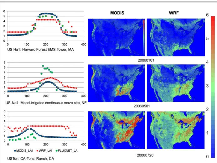
Figure 2.1. PX LSM WRF, MODIS, and FLUNXET LAI comparisons. The LAI graphs on the left have LAI on the vertical axis and day of
year with 1 for Jan. 1, 2006 on the horizontal axis... 13 Figure 2.2. PX WRF vegetation cover and MODIS gridded FPAR used
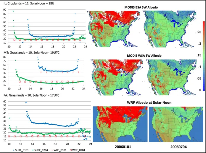
as the surrogate of vegetation cover fraction for 2006-08-10. ... 15 Figure 2.3. PX WRF, SURFRAD, and MODIS albedo comparisons.
The albedo graphs on the left have albedo (%) on the vertical axis
and local time zone hour of day on the horizontal axis. ... 17 Figure 2.4. Statistical metrics (y axis) vs. observation range (x axis) for
2 m T (K) and Q (g kg-1) over the period from Aug. 10 – Sept. 9, 2006. The top plots are for 2 m T and the bottom for 2 m Q. The two plots on the left are from the base case meteorology and the
plots on the right are from the LAI-FPAR case. ... 26 Figure 2.5. Mean Bias Difference (LAI-FPAR Case – Base Case) spatial
and histogram plots over the period from Aug. 10 – Sept. 9, 2006.
The top row is for 2 m T (K) and the bottom row is for Q(g kg-1). ... 27 Figure 2.6. ASOS measurement site 2 m T (K) and Q (g kg-1) time series
comparison for the period from Aug. 15-25, 2006. KDAG site is in black line, LAI-FPAR case is in red line, and base case is in blue line. Site grid cell has VF 0.669 and LAI 2.282 for the base case and
VF 0.186 and LAI 1.258 for the LAI-FPAR case. ... 29 Figure 2.7. ASOS measurement site 2 m T (K) and Q (g kg-1) time series
comparison for the period from Aug. 15-25, 2006. KPGA site is in black line, LAI-FPAR case is in red line, and base case is in blue line. Site grid cell has VF 0.580 and LAI 1.918 for the base case and
VF 0.105 and LAI 1.227 for the LAI-FPAR case. ... 30 Figure 2.8. Mean bias difference (CMAQ LAI-FPAR-Albedo Case –
Base Case) spatial plot for daily maximum 8-hour average O3 (ppb)
over the period from Aug. 10-30, 2006. ... 32 Figure 2.9. Mean bias (MB) and root mean square error (RMSE) of
daily maximum 8-hour average O3 (ppb) over the binned
observation range for CMAQ LAI-FPAR-Albedo Case (in red) and Base Case (in blue) from Aug. 10-30, 2006. Line length is for the range of MB and RMSE, triangle for the median, and asterisk for
the mean... 32 Figure 2.10. Tonzi-CA FLUXNET measurement latent and sensible
xiii
FLUXNET site is in blue line, base case is in red line, and
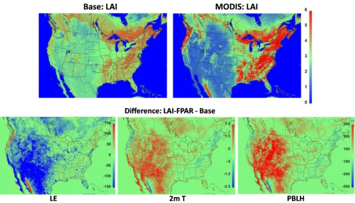
LAI-FPAR case is in green line. ... 34 Figure 2.11. LAI for 20Z, August 10, 2006 and average differences of
latent heat (W m-2), 2 m T (K), and PBLH (m) between the LAI-FPAR case and base case for 20 UTC from August 10 to September
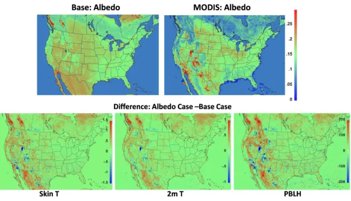
09, 2006. ... 35 Figure 2.12. Albedo (fraction) for 20Z, August 10, 2006 and average
differences of surface skin T (K), 2 m T (K) and PBLH (m) between the albedo case and the base case for 20 UTC from August 10 to
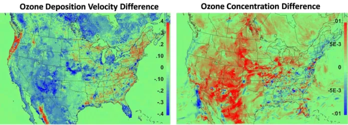
September 09, 2006. ... 36 Figure 2.13. Difference of ozone deposition velocity (cm s-1) and ozone
concentration (ppmV) at the surface layer between the CMAQ
LAI-FPAR-albedo case and base case for 20Z, August 10, 2006. ... 38 Figure 2.14. Monthly precipitation difference (mm) of the LAI-FPAR
case and the base case from the PRISM precipitation for August
2006. ... 39 Figure 2.15. Mean bias difference of precipitation (mm) between the
LAI-FPAR-Albedo case and the base case at the National
Atmospheric Deposition Program (NADP) sites for August. ... 40 Figure 2.16. Mean bias difference of NH4 wet deposition (kg ha-1)
between the LAI-FPAR-Albedo case and the base case at the National Atmospheric Deposition Program (NADP) sites for
August... 41 Figure 3.1. Original (F1_old) and improved (F1_new) F1 functions with
incoming solar radiation Rg (W m-2) in the PX LSM Jarvis stomatal
conductance function. F1 (scalar) represents the impact of Rg on
stomatal conductance or photosynthesis when other factors are at optimal conditions. F1 is computed for broadleaf forest type with assumed Rstmin=200 (s m-1), Rstmax=5000.0 (s m-1), and LAI=5.5(m2
m-2). ... 62 Figure 3.2. Comparison of soil resistances computed based four
formulations described by Sakaguchi and Zeng [2009], Sellers et al. [1992], Lee and Pielke [1992], and Kondo et al. [1990] for sandy loam soil. Soil resistances are computed with wfc=0.195 m3 m-3,
wsat=0.435 m3 m-3, wres=0.01 m3 m-3, b=4.9, d1=1.75 cm, and Raw=50
s m-1. ... 66 Figure 3.3. Diurnal domain-wide statistical metrics (y axis) for
xiv
with UTC hours. The left column is for the previous WRF [Ran et al., 2015] and the right column is for the updated WRF. The top row is for the base case simulations without MODIS input and the
bottom row is for the MODIS case simulations. ... 73 Figure 3.4. Diurnal domain-wide statistical metrics (y axis) for
simulated 2 m Q (g kg-1) against MADIS observations over the period from 10 August to 9 September 2006. The x axis is time of day with UTC hours. The left column is for the previous WRF [Ran et al., 2015] and the right column is for the updated WRF. The top row is for the base case simulations without MODIS input and the
bottom row is for the MODIS case simulations. ... 74 Figure 3.5. Spatial plots for the differences of the absolute mean biases
(MODIS case – base case) for WRF simulations against MADIS observation sites over the period from 10 August to 9 September 2006. The left column is for the previous WRF [Ran et al., 2015] and the right column is for the updated WRF. The top row is for 2
m T (K) and the bottom row is for 2 m Q (g kg-1). ... 76 Figure 3.6. Spatial plots of statistical metrics for WRF simulations with
MODIS input against MADIS observation sites over the period from 10 August to 9 September 2006. The left column is for the mean bias of the MODIS case using the previous model [Ran et al., 2015], the middle column is for the difference of the absolute mean biases between the MODIS cases using the updated model and previous model, and the right column is for the difference of the mean absolute errors. The top row is for 2 m T (K) and the bottom row is
for 2 m Q (g kg-1)... 77 Figure 3.7. Evaluation of daily maximum 8 h average O3 (ppb)
simulated with MODIS input using the updated WRF/CMAQ and the previous WRF/CMAQ [Ran et al., 2015] over the period from 10 to 30 August 2006 against the EPA AQS sites. The top plot displays mean of daily maximum 8 h average O3 from the previous
system (blue line), updated system (red line) and all AQS sites (black line). The spatial plot shows the difference of absolute mean bias for daily maximum 8 h average O3 between the updated system
and previous system. ... 79 Figure 3.8. Mean bias (MB, left plot) and root-mean-square error
(RMSE, right plot) of daily maximum 8 h average O3 (ppb)
xv
MB and RMSE, triangle and circle for the median, and asterisk for
the mean... 80 Figure 3.9. 2006 monthly and daily average statistical metrics for 2 m Q
(g kg-1, y axis) domain-wide for the base and MODIS WRF
simulations against MADIS observations. The left graph is for the monthly averages of the mean biases and mean absolute errors. The right graph is for the daily average of the mean biases and root mean
square errors. ... 82 Figure 3.10. April 2006 LAI (m2 m-2), latent heat (W m-2), and 2 m Q (g
kg-1) spatial evaluation. The top row is for the monthly average LAI from the MODIS case (top left) and base case (top middle) and for the difference of the average LAI between the two cases (top right). The bottom left plot is for the difference of the monthly average latent heat between the two cases for 20 UTC. The bottom middle plot is for the mean bias of 2 m Q from the MODIS case against MADIS observations. The bottom right plot is the difference of
absolute mean bias for 2 m Q between the two cases. ... 85 Figure 3.11. May 2006 LAI (m2 m-2), latent heat (W m-2), and 2 m Q (g
kg-1) spatial evaluation. Plot descriptions are the same as those in
the figure 3.10 caption. ... 86 Figure 3.12. June 2006 LAI (m2 m-2), latent heat (W m-2), and 2 m Q (g
kg-1) spatial evaluation. Plot descriptions are the same as those in
the figure 3.10 caption. ... 88 Figure 3.13. August 2006 LAI (m2 m-2), latent heat (W m-2), and 2 m Q
(g kg-1) spatial evaluation. Plot descriptions are the same as those in
the figure 3.10 caption. ... 88 Figure 3.14. October 2006 LAI (m2 m-2), latent heat (W m-2), and 2 m Q
(g kg-1) spatial evaluation. Plot descriptions are the same as those in
the figure 3.10 caption. ... 90 Figure 3.15. Monthly average difference of LAI (m2 m-2), ozone
deposition velocity (cm s-1), and ozone concentration (ppmV) at the surface layer between the MODIS case and base case for 20 UTC
over April, August, and October 2006. ... 92 Figure 3.16. Evaluation of daily maximum 8 h average O3 (ppb)
simulated from the base and MODIS case WRF/CMAQ over August 2006 again the EPA AQS sites. The top plot displays mean of daily maximum 8 h average O3 from the base case (blue line),
xvi
maximum 8 h average O3 between the MODIS case and the base
case. ... 94 Figure 4.1. Evaluation of daily maximum 8 hour average O3 (ppb)
simulated from an improved WRF/CMAQ with/without MODIS vegetation and albedo input over August 2006 against the EPA Air Quality System (AQS) sites. The top plot displays mean of daily maximum 8 hour average O3 from the base model (blue line), the
model with MODIS input (red line) and all AQS sites (black line). The bottom plot is the mean bias spatial plot for daily maximum 8 hour average O3 simulated from the base model without MODIS
input. The base model’s vegetation is computed from vegetation parameters prescribed in land use category lookup tables using
equations 2 and 3 in Ran et al. [2015a]. ... 111 Figure 4.2. Canopy scaling and radiative transfer parameters plots. The
top row plots are the leaf canopy fraction (top left) and the absorbed PAR fraction to the incident PAR (top right) for the sunlit and shaded leaves. The bottom row plots are the sunlit and shaded LAI (bottom left) with changing zenith angle and the direct and diffuse extinction coefficients (bottom right) as a function of zenith angle and LAI. Parameters are computed based on US-Ha1 data on 13 June 2006 at 12pm with longitude = W 72.1715, latitude = N
42.5378, LAI = 4 (m2 m-2), zenith angle = 20°, x = 1 (spherical leaf), αleaf = 0.8 for PAR (leaf absorptivity), and αleaf = 0.2 for NIR, forest
floor reflectance = 0.10... 128 Figure 4.3. Transpiration as a function of deep soil moisture (F2 function
by eq. 4.3), computed based on US-Ha1 data on 2 July 2006 at 12pm with changing deep soil moisture (w2). The box model uses
the loam soil properties (wfc = 0.24 m3 m-3, wsat = 0.451 m3 m-3,
wwlt=0.155 m3 m-3) from the box PX LSM for the site. ... 131
Figure 4.4. Diurnal median comparisons of the estimated latent heat (LH) from the photosynthesis approaches used by JULES [Clark et al., 2011], Song et al. [2009], and photosynthesis-based PX LSM (PX PSN) to compute three potential assimilation rates (Ac, Aj, and
Ae) in comparison with LH from the PX LSM Jarvis approach
[Pleim and Xiu, 1995] and the observation data at the FLUXNET Harvard Forest US-Ha1 site [Urbanski et al., 2007]. The broadleaf C3 plant simulations are conducted in the PX box model using July
2006 US-Ha1 standardized L2 data with canopy height = 25 m, x = 1 (spherical leaf), αleaf = 0.8 for PAR (leaf absorptivity), αleaf = 0.2
for NIR, forest floor reflectance = 0.10, VCMAX25_0= 30×10-6 mol m-2
s-1, kn = 0.17, Tlow = 0.0 °C, Tup = 36 °C, leaf scattering coefficient
0.15, quantum yield ε = 0.08 (mol CO2 mol-1
photon), and Jarvis
xvii
Figure 4.5. Stomatal conductance (m s-1, left) and ozone deposition velocity (m s-1, right) computed from the PX Jarvis and
photosynthesis-based approach from 2 to 11 July 2006 with the
modeling parameters described in the figure 4.4 caption. ... 133 Figure 4.6. Missouri Ozark/US-Moz site LH diurnal median
comparisons. LH is simulated with the photosynthesis-based and Jarvis approaches using the observed LAI (left plot) and the MODIS LAI (right plot) from 9 July (190) - 14 November (318) 2006. The observed LAI from the site 2006 biological data and processed 2006 MODIS LAI for the deciduous broadleaf land cover type at the 12 km CMAQ grid cell are displayed in the middle plot. Soil moisture
measurements at 100 cm deep are used. ... 138 Figure 4.7. Missouri Ozark/US-Moz site scatter plot comparisons of
daily total LH estimations. ... 139 Figure 4.8. Wind River Field Station/US-Wrc site LH diurnal medium
comparisons. LH is simulated with the photosynthesis-based and Jarvis approaches using the observed LAI (left plot) and the MODIS LAI (right plot) from 7 January (7) - 28 November (333) 2008. The observed LAI of the C3 vegetation from the study by Thomas and
Winner [2000] and processed 2006 MODIS LAI for the evergreen needleleaf land cover type at the 12 km CMAQ grid cell are
displayed in the middle plot. Soil moisture measurements at 40 cm
deep are used. ... 143 Figure 4.9. Fermi Prairie/US-IB2 site LH diurnal median comparisons.
LH is simulated with the photosynthesis-based and Jarvis
approaches using the observed LAI (left plot) and the MODIS LAI (right plot) from 22 May (142) - 20 September (263) 2006. The observed LAI of the C4 grassland from the site 2006 biological data
and processed 2006 MODIS LAI for the grassland land cover type at the 12 km CMAQ grid cell are displayed in the middle plot. Soil
moisture measurements at 25 cm deep are used. ... 145 Figure 4.10. Fermi Prairie/US-IB2 site scatter plot comparisons of daily
total LH estimations. ... 146 Figure 4.11. Mead Irrigated Rotation/US-Ne2 site LH diurnal median
comparisons. LH is simulated with the photosynthesis-based and Jarvis approaches using the observed LAI (left plot) and the MODIS LAI (right plot) from 12 June (163) - 5 October (278) 2006. The observed LAI of C3 soybean from the site 2006 biological data and
processed 2006 MODIS LAI for the cropland land cover type at the 12 km CMAQ grid cell are displayed in the middle plot. Soil
xviii
Figure 4.12. Mead Irrigated Rotation/US-Ne2 site scatter plot
comparisons of daily total LH estimations. ... 149 Figure 4.13. Duke Forest Open Field/US-Dk1 site LH diurnal median
(left plot) and selected hourly (right plot) comparisons. Simulations are conducted based on LAI = 3 (m2 m-2) and other parameters listed in table 4.1 for the periods of 17 May (day 137) to 18 June (day 169) and 18 to 28 September (day 261 to 271) 2013 with
measurements. Hourly display is for 25 to 30 May 2013 (day 145 to
150). ... 151 Figure 4.14. Duke Forest Open Field/US-Dk1 site diurnal median
comparisons for estimated stomatal conductance (cm s-1, left plot), ozone deposition velocity (cm s-1, middle plot), and ozone flux (μg
m-2 s-1, right plot). ... 152 Figure 4.15. Duke Forest Open Field/US-Dk1 site scatter plot
comparisons of daily total LH and ozone flux estimations. ... 152 Figure 4.16. Duke Forest Open Field/US-Dk2 site hourly comparisons
for estimated stomatal conductance (cm s-1, left plot), ozone
deposition velocity (cm s-1, middle plot), and ozone flux (μg m-2 s-1,
xix
LIST OF ABBREVIATIONS ACM2 Asymmetric Convective Model version 2
AE6 Aerosol 6 module
AMET Atmospheric Model Evaluation Tool
APAR Absorbed photosynthetically active radiation
AQ Air quality
AQS Air Quality System
AQMEII Air Quality Model Evaluation International Initiative ASOS Automated Surface Observing System
AZ Arizona
BIAS Mean bias
BRDF Bidirectional reflectance distribution function
BWB the Ball-Woodrow-Berry
C3 C3 carbon fixation in photosynthesis
C4 C4 carbon fixation in photosynthesis
CA California
“CAA” Clean Air Act
CESM Community Earth System Model
CB05 Carbon Bond mechanism
CLM Community Land Model
cm Centimeter
CO Carbon monoxide
CO2 Carbon dioxide
xx
DAMB Difference of absolute mean biases DMAE Difference of mean absolute errors E, ET Evapotranspiration
EPA Environmental Protection Agency
FLUXNET Flux Network
FPAR Fraction of absorbed photosynthetically active radiation
g Grams
GCM Global climate model
GEOV1 GEOLAND2 Version 1
GHGs Greenhouse gases
GLASS Global Land Surface Satellite GLOBMAP Global mapping
ha Hectares
hPA Hectopascal
IGBP International Geosphere-Biosphere Programme ISBA Interactions Soil Biosphere Atmosphere
JRC-TIP Joint Research Centre Two-stream Inversion Package JULES Joint UK Land Environment Simulator
K Kevin
KDAG ASOS site at the Barstow-Daggett airport, CA, US
KF2 Kain–Fritsch 2
kg Kilograms
KPGA ASOS site at the Page Municipal Airport, Arizona, US
L2 Level 2
xxi
LAI Leaf area index
LBC Lateral boundary conditions
LE, LH Latent heat
LSM Land surface model
m Meter
MACC-II Monitoring Atmospheric Composition and Climate Interim Implementation
MADIS Meteorological Assimilation Data Ingest System
MAE Mean absolute error
MB Mean bias
MCD43A1 MODIS BRDF/Albedo Model Parameters product MCD43A2 MODIS BRDF/Albedo Quality product
MCD43A3 MODIS Albedo product at 500m resolution MCIP Meteorology-Chemistry Interface Processor
mm Millimetre
MOD15A2GFS Gap-Filled, smoothed MODIS LAI/FPAR products MODIS Moderate Resolution Imaging Spectroradiometer MOST Monin-Obukov similarity theory
NACP North American Carbon Program
NADP National Atmospheric Deposition Program
NAM North American Model
λE Latent heat (W m-2)
xxii
netCDF Network Common Data Form
NH3 Ammonia
NH4 Ammonium
NIR Near infrared radiation
NLCD National Land Cover Database
NMB Normalized mean bias
NME Normalized mean error
NO2 Nitrogen dioxide
NOAA Oceanic and Atmospheric Administration
NOx Nitrogen oxides
O3 Ozone
OBS Observation
PAR Photosynthetically active (visible) radiation
PBL Planetary boundary layer
PBLH Planetary boundary layer height
PEP Phosphoenolpyruvate
PFT Plant function type
PM2.5 Fine particulate matter
ppb Parts per billion
ppmV Parts per million by volume
PRISM Parameter-elevation Relationships on Independent Slopes Model
PX Pleim-Xiu
PX PSN Photosynthesis-based stomatal conductance model for the PX LSM RAMS Regional Atmospheric Modeling System
xxiii
RRTMG WRF Rapid Radiative Transfer Model for GCMs
SH Sensible heat
SFDDA Surface four-dimensional data assimilation
SO2 Sulfur dioxide
StDev Standard deviation
SURFRAD SURFace RADiation Budget Measurement
SW South west
SZA Solar zenith angle
μg Microgram
UK United Kingdom
U.S. United States
US-Dk1 U.S. FLUXNET Duke Forest Open Field in North Carolina US-IB2 U.S. FLUXNET Fermi Prairie in Illinois
US-Ha1 U.S. FLUXNET Harvard Forest in Massachusetts US-MOz U.S. FLUXNET Missouri Ozark
US-Ne1 U.S. FLUXNET Mead irrigated maize in Nebraska US-Ne2 U.S. FLUXNET Mead irrigated rotation in Nebraska US-Ton U.S. FLUXNET Tonzi Ranch in California
US-Wrc U.S. FLUXNET Wind River Field Station in Washington
UV Ultraviolet
U/V Wind u (zonal velocity) and v (meridional velocity) components UTC Coordinated Universal Time
VF Vegetation fraction
xxiv WRF Weather Research and Forecast
WS Wind speed
xxv
LIST OF SYMBOLES A Leaf CO2 assimilation rate (mol CO2 m-2 s-1)
Ac Leaf CO2 assimilation rate limited by Rubisco (mol CO2 m-2 s-1)
Acnet Net CO2 assimilation rate at the canopy scale (mol CO2 m-2 s-1)
Ae Leaf CO2 assimilation rate limited by transport of photosynthetic products
for C3 plants or phosphoenolpyruvate (PEP) carboxylase limitation for C4
plants (mol CO2 m-2 s-1)
Ai Smoothed minimum of Ac and Aj leaf CO2 assimilation rate (mol CO2 m-2
s-1)
Aj Leaf CO2 assimilation rate limited by light (mol CO2 m-2 s-1)
α Constant (set to 1) in surface soil layer temperature Tg computation
αBSA Black-sky albedo (direct)
αBLUE Blue-sky albedo (actual)
αleaf Leaf absorptivity
αWSA White-sky albedo (diffuse)
Anet Net CO2 assimilation rate at the leaf scale (mol CO2 m-2 s-1)
Anet_shd Net CO2 assimilation rate at the shaded leaf scale (mol CO2 m-2 s-1)
Anet_sun Net CO2 assimilation rate at the sunlit leaf scale (mol CO2 m-2 s-1)
ANIR Absorbed NIR at the leaf (sunlit or shaded) (W m-2) APAR Absorbed PAR at the leaf (sunlit or shaded) (W m-2)
b Slope of the retention curve varying with soil texture in soil resistance computation
β Factor of the volumetric water content of the top soil layer and at field capacity
cc CO2 compensation point in the absence of non-photorespiratory
xxvi
ch Volumetric heat capacity (J m-3 k-1 )
ci CO2 partial pressure inside the leaf stomata (Pa)
cs CO2 partial pressure at the leaf surface (Pa)
Ct Coefficient that is inversely proportional to heat capacity (K m2 J-1)
Cg Ct for the soil surface in a grid cell (K m2 J-1)
Cv Ctfor vegetation in a grid cell and set to 1.2×10⁻⁵ (K m2 J-1)
d Damping depth of the diurnal temperature wave (m) d1 Top soil layer thickness which is set to 1.75 cm
D Diffuse radiation fraction
D0 Molecular diffusion coefficient of water vapor in the atmosphere and is set
to a constant 2.59 × 10⁻⁵ (m2 s-1)
Ds Reduced soil vapor diffusivity soil for soil resistance computation (m2 s-1)
e Constant 2.71828
Eg Evaporation from the soil surface (kg m-2 s-1)
ei Saturation vapor pressure (Pa) inside the leaf stomata at the vegetation
surface temperature (Ts)
ε Quantum yield in photosynthesis (mol CO2 mol-1 photon)
εj Computed electron transport quantum use efficiency in photosynthesis
(mol CO2 mol-1 photon)
es Vapor pressure at the leaf surface (Pa)
Ess Evaporation from the bare soil surface (kg m-2 s-1)
ETc Evapotranspiration from the canopy (kg m-2 s-1)
Evs Evaporation from the vegetation surface (kg m-2 s-1)
F1 Fractional degree (0 to 1) of stomatal closure caused by photosynthetically
xxvii
F2 Fractional degree (0 to 1) of stomatal closure caused by Root-depth (1 m)
volumetric soil moisture (w2)
F3 Fractional degree (0 to 1) of stomatal closure caused by relative humidity
at the leaf surface (RHs)
F4 Fractional degree (0 to 1) of stomatal closure caused by air temperature in
the canopy (Tic)
fdr Dark respiration coefficient which is set as 0.015 for C3 plants and 0.025
for C4 plants following JULES [Clark et al., 2011]
fiso, fvol, fgeo MODIS BRDF/albedo anisotropy three parameters (Isotropic, RossThick,
LiSparseR)
fLW Scaling factor of the longwave radiation to the canopy
fseas Seasonal adjustment factor for LAI and VF
G Ground heat flux (W m-2)
Gc Canopy stomatal conductance (m s-1)
g0 Minimum leaf stomatal conductance (mol CO2 m-2 s-1). Set 0.01 for C3
plants and 0.04 for C4 plants.
g0iso, g1iso, g2iso MODIS BRDF/albedo Isotropic constants
g0vol, g1vol, g2vol MODIS BRDF/albedo RossThick constants
g0geo, g1geo, g2geo MODIS BRDF/albedo LiSparseR constants
giso, gvol, ggeo Computed MODIS BRDF/albedo anisotropy three functions (Isotropic,
RossThick, LiSparseR) with solar zenith angle gst Leaf stomatal conductance for CO2 (mol CO2 m-2 s-1)
gst_shd Shaded leaf stomatal conductance for CO2 (mol CO2 m-2 s-1)
gst_sun Sunlit leaf stomatal conductance for CO2 (mol CO2 m-2 s-1)
gstw_sun Sunlit leaf stomatal conductance for water vapor (m s-1)
Gst Canopy stomatal conductance for water vapor (m s-1)
xxviii H Sensible heat flux (W m-2)
Iapar Absorbed photosynthetically active radiation (APAR) by the leaf (mol
photon m-2 s-1)
J Rate of electron transport in photosynthesis (mol electron m-2 s-1)
Jmax Maximum electron transport rate in photosynthesis (mol electron m-2 s-1)
Kc Michaelis-Menten constant for CO2 defined by equation 9 by Clark et al.
[2011] (Pa)
Kdif Extinction (attenuation) coefficient for diffuse light within the canopy
Kdir Extinction coefficient for direct beam within the canopy
Kn Foliage nitrogen decay coefficient and defined as 0.17 [Bonan et al., 2011]
Ko Michaelis-Menten constant for O2 defined by equation 10 by Clark et al.
[2011] (Pa)
LAI Leaf area index (m2 m-2)
LAImin Minimum leaf area index (m2 m-2)
LAImax Maximum leaf area index (m2 m-2)
LAIshd LAI for the shaded leaves (m2 m-2)
LAIsun LAI for the sunlit leaves (m2 m-2)
Ls Estimated soil dry layer path length (m) in soil resistance computation
LWair Long wave radiation from air (W m-2)
LWcanopy Long wave radiation from the canopy (W m-2)
LWfloor Long wave radiation from the floor (W m-2)
λ Latent heat of evaporation (k J kg-1) λt Thermal conductivity (W m-2 K-1)
λE Latent heat flux (W m-2)
mg Plant-type parameter which is 9 for C3 plants and 4 for C4 plants
xxix NMB Normalized mean bias NME Normalized mean error
Oa Partial pressure of atmospheric oxygen (Pa)
Oi Observed daily total flux at day i
Pa Atmospheric pressure (Pa)
PAR Photosynthetically active radiation (W m-2)
π Pi constant
Q Mixing ratio (g kg-1)
qa Water vapor mixing ratio at the lowest atmospheric layer (kg kg-1)
qs(Ts_sun) Saturated mixing ratio for water vapor at the sunlit leaf temperature Ts_sun
(kg kg-1)
qsat(Ts) Saturated water vapor mixing ratio (kg kg-1) at the soil surface temperature
(Ts)
Ra Aerodynamic resistance (s m-1)
Raw Equal to Ra + Rbw (s m-1)
Rbw Quasi-laminar boundary layer resistance for water vapor (s m-1)
Rg Incoming solar radiation at the surface (W m-2)
Rgl Limiting factor with 30 (W m-2) for forest types and 100 (W m-2) for
other vegetation types in computing F1
RHs Relative humidity at the leaf surface
Rnet Net radiation for the sunlit or shaded leaf (W m-2)
Rs Soil resistance (s m-1)
ρa Density of dry air (kg m-3)
Rstmin, Rstmax Minimum and maximum stomatal resistances (s m-1)
xxx
T Temperature (K)
T2 Deep soil layer (1 m) temperature (K)
τ Diurnal time scale (s)
τdir Transmittance of beam radiation for non-horizontal scattering leaves
τdif Transmittance for diffuse radiation over the entire upper hemisphere
Tg Surface soil layer (1 cm) temperature (K)
Tic Air temperature in the canopy (K)
Tlow Lower limit of the optimal temperature range defined for PFT types in
JULES [Clark et al., 2011] (°C) θsun Solar zenith angle (radians)
TRc Transpiration from the canopy (kg m-2 s-1)
TRc_shd Transpiration from the shaded leaf canopy (kg m-2 s-1)
TRc_sun Transpiration from the sunlit leaf canopy (kg m-2 s-1)
Ts Canopy leaf surface temperature (°C)
Tssl Soil surface temperature (K)
Tup Upper limit of the optimal temperature range defined for PFT types in
JULES [Clark et al., 2011] (°C) u* Friction velocity (m s-1)
Vcmax Maximum rate of carboxylation of Rubisco (mol CO2 m-2 s-1)
Vcmax25 Vcmax at 25°C (mol CO2 m-2 s-1)
Vcmax25_0 Vcmax25 at the top of the canopy (mol CO2 m-2 s-1)
vegF Vegetation fraction for a grid cell VFmin Minimum vegetation fraction
xxxi
w Parameter which controls the concavity of the curve and is set to 5 for the exponential shape in soil resistance computation
w2 Root-depth (1 m) volumetric soil moisture (m3 m-3)
w2avl Available volumetric soil water content at root depth (m3 m-3)
w2 mxav Maximum available volumetric soil water content at root depth (m3 m-3)
wfc Volumetric soil water content at field capacity (m3 m-3)
wg Volumetric soil water content of the top soil layer (m3 m-3)
wsat Volumetric soil water content at saturation (m3 m-3)
wres Volumetric soil residual water content (m3 m-3)
wwlt Volumetric soil water content at the wilting point (m3 m-3)
1
CHAPTER 1: INTRODUCTION 1.1 Introduction
The combined meteorology and air quality modeling system composed of the Weather Research and Forecast (WRF) model and Community Multiscale Air Quality (CMAQ) model is an important decision support tool that is used in research and regulatory decisions related to emission, meteorology, climate, and chemical transport around the world. The land surface model (LSM) is an important component in WRF/CMAQ for simulating the exchange of heat, moisture, momentum, and trace atmospheric chemicals between the land surface and the atmosphere. Vegetation transpiration is a crucial component in the surface energy budget and the water and carbon cycles of LSMs. Vegetation is also a source and sink of many atmospheric chemicals such as O3 and volatile organic compounds (VOCs).
The Pleim-Xiu (PX) LSM is commonly used in retrospective WRF/CMAQ simulations for research and policy making. Different from LSMs in climate earth system models with complex dynamic vegetation processes, the LSM has much simpler vegetation treatment with a big-leaf empirical function stomatal conductance approach to model vegetation transpiration and pollutant deposition. Surface characteristics including vegetation parameters and surface albedo are specified in LSM land use look-up tables and plant phenological dynamics are modeled using simple time and temperature dependent functions. With data assimilation the LSM has
demonstrated strong capabilities in modeling the land surface processes for meteorology and air quality modeling. However, with increased needs to conduct year-long retrospective
2
changes (e.g. phenology) and disturbances (e.g. fires, storm damages). In addition, lacking a biochemically-based photosynthesis-conductance scheme could limit not only the model’s dynamic responses to environmental conditions such as temperature, air pollutants (e.g. O3) and
CO2 concentration but also their applications in assessing the coupling effects of air quality and
vegetation productivity in changing climate. 1.2 Objective
The objective of this research is to improve land surface processes in retrospective WRF/CMAQ modeling by:
1) Incorporating satellite-derived temporal vegetation and albedo data for faithful surface representation and
2) Advancing the vegetation processes with a biochemically-based photosynthesis-stomatal conductance approach.
The two components of this research are synergistic because accurate vegetation
representation is essential for estimating canopy CO2 assimilation and stomatal conductance
using the biochemically-based photosynthesis approach. As WRF/CMAQ is an important decision support tool for mitigating harmful effects of air pollution on human health and ecosystems, improving the tool through development of more advanced science processes and incorporation of satellite observations will have direct benefit to society.
1.3 Method
3
and atmospheric chemistry. The research focuses on improving the land surface representation and vegetation processes in the PX LSM through the following three incremental studies:
1) Evaluate the sensitivity of WRF/CMAQ with PX LSM to MODIS LAI, FPAR, and albedo,
2) Assess impacts of MODIS input on seasonality during a yearlong simulation using an updated WRF/CMAQ modeling system, and
3) Develop, test, and evaluate a coupled photosynthesis-based stomatal conductance approach in PX LSM to advance the vegetation processes in WRF/CMAQ with direct connection to CO2 level and vegetation productivity.
The science questions to be addressed by this research are:
1) How well does current WRF/CMAQ with PX LSM represent vegetation and surface albedo?
2) How does the WRF/CMAQ with PX LSM respond to the more realistic surface representation from MODIS input?
3) Can the WRF/CMAQ model be modified to produce improved results when using the MODIS input?
4) Can phenology from MODIS input help improve multi-seasonal WRF/CMAQ simulations?
5) Can a coupled photosynthesis-stomatal conductance approach perform as well as the PX Jarvis stomatal conductance approach?
4
The three incremental studies are presented in chapters 2, 3, and 4 in sequence as
independent papers. Research summary, future work and significance are presented in the last Chapter.
1.4 Expected Results
The research results in an advanced WRF/CMAQ model including MODIS vegetation and albedo input and a coupled photosynthesis and stomatal conductance approach incorporated into the PX LSM. Assimilating MODIS vegetation and albedo into the modeling system can provide up-to-date landscape information with more accurate phenology and disturbance
representation. The photosynthesis-based stomatal conductance approach provides responses of C3 and C4 plants to environmental conditions through biochemically-based processes associated
with CO2 assimilation. The realistic surface representation from satellite observations and
5
CHAPTER 2: SENSITIVITY OF THE WEATHER RESEARCH AND
FORECAST/COMMUNITY MULTISCALE AIR QUALITY MODELING SYSTEM TO MODIS LAI, FPAR, AND ALBEDO1
Abstract
This study aims to improve land surface processes in a retrospective meteorology and air quality modeling system through the use of Moderate Resolution Imaging Spectroradiometer (MODIS) vegetation and albedo products for more realistic vegetation and surface representation. MODIS leaf area index (LAI), fraction of absorbed photosynthetically active radiation (FPAR), and albedo are incorporated into the Pleim-Xiu land surface model (PX LSM) used in a
combined meteorology and air quality modeling system. The current PX LSM intentionally exaggerates vegetation coverage and LAI in western drylands so that its soil moisture nudging scheme is more effective in simulating surface temperature and mixing ratio. Reduced
vegetation coverage from the PX LSM with MODIS input results in hotter and dryer daytime conditions with reduced ozone dry deposition velocities in much of western North America. Evaluations of the new system indicate greater error and bias in temperature, but reduced error and bias in moisture with the MODIS vegetation input. Hotter daytime temperatures and reduced dry deposition result in greater ozone concentrations in the western arid regions even with deeper boundary layer depths. MODIS albedo has much less impact on the meteorology simulations than MODIS LAI and FPAR. The MODIS vegetation and albedo input does not
1
6
have much influence in the east where differences in vegetation and albedo parameters are less extreme. Evaluation results showing increased temperature errors with more accurate
representation of vegetation suggests that improvements are needed in the model surface physics, particularly the soil processes in the PX LSM.
2.1 Introduction
Degraded air quality (AQ) is a persistent environmental problem that causes serious health, ecological, and climate consequences (e.g. mortality, eutrophication, biodiversity loss, climate forcing). To improve AQ and mitigate the deleterious effects on human health,
ecosystems and climate, policy makers and scientists rely on comprehensive computer modeling systems that simulate emissions, transport, chemistry, and deposition of air pollutants to design emission control strategies for achieving healthy sustainable AQ [Cohan et al., 2007]. The combined meteorology and air quality modeling system WRF/CMAQ - composed of the National Center for Atmospheric Research (NCAR) Weather Research and Forecast (WRF) model [Skamarock et al., 2008] and the United States (US) Environmental Protection Agency (EPA) Community Multiscale Air Quality (CMAQ) model [Byun and Schere, 2006] is an important decision support tool that is used to help understand the chemical and physical processes involved in AQ degradation and to develop policy to mitigate harmful effects of air pollution on human health and the environment around the world [Isakov et al., 2007; Wang et al., 2010; Compton et al., 2011]. Improving spatial and temporal distributions of modeled air pollutant concentrations and deposition, particularly O3, PM2.5, and NH4, will help reduce the
7
emissions, transport, photolysis rates, photochemistry, and land surface exchange may contribute to errors in the current modeling system. Our research focuses on improving land surface model (LSM) processes in the WRF/CMAQ, which includes both meteorological (heat, moisture, and momentum) and chemical (dry deposition and bi-directional exchange) surface fluxes, through using satellite-derived land surface data.
The two commonly used LSMs for meso-scale WRF meteorology modeling are the Noah [Chen and Dudhia, 2001] and PX LSMs [Pleim and Xiu, 1995; Xiu and Pleim, 2001]. Unlike climate LSMs (e.g. Oleson et al., 2013; Clark et al., 2011) with complex hydrology and dynamic vegetation coupled with climate to model processes over decadal to century future periods, these two LSMs rely heavily on data initialization and assimilation for high accuracy over relative short periods (days to years). Thus, both the LSMs have simple canopy treatments with a big-leaf empirical function stomatal conductance following the approach described by Noilhan and Planton [1989] as well as simple soil hydrology and snow processes. When applied
retrospectively for long term simulations, such as for full years, accurate Noah WRF simulations rely on frequent (e.g. every 2-5 days) re-start of simulations with re-initialized soil conditions [e.g. Hogrefe et al., 2014] while the PX LSM uses continuous data assimilation for dynamic nudging of soil moisture [Pleim and Xiu, 2003] and temperature [Pleim and Gilliam, 2009] to optimize surface fluxes. The PX LSM is mainly designed for air quality simulations using the WRF/CMAQ system where the WRF LSM parameters (e.g. stomatal and aerodynamic
resistances) are consistently used in the AQ dry deposition model.
8
Rogers et al., 2013; Hogrefe et al., 2014]. At the start of an extended run, the soil moisture fields can be very quickly and effectively spun up from simple generic initializations (e.g. from moisture availability factors by land use type) in about 5 days [Pleim and Gilliam, 2009]. To ensure good model performance when using the PX LSM, the key is to configure the WRF simulation with the PX LSM indirect soil moisture and temperature nudging. For example, Miao et al. [2007] described a modeling study comparing the Noah and PX LSMs implemented in MM5 and concluded that soil moisture initialization is crucial for the PX LSM performance. However, since they did not use data assimilation in their study the soil moisture nudging scheme was not activated in the simulation with the PX LSM scheme. The PX LSM dynamic continuous data assimilation has the strength to continuously and effectively adjust soil temperature and moisture without re-starting the simulation for reducing error growth in atmospheric variables such as 2 m temperature (T) and mixing ratio (Q) [Pleim and Xiu, 2003; Pleim and Gilliam, 2009]. However, it has the drawback that the assimilation may compensate and mask errors in model physics and it may cause changes in soil moisture when the
atmospheric model’s temperature and relative humidity errors are not related to surface fluxes. In addition, the PX LSM treats modeling grids with land cover fractions instead of the dominant land cover type in each grid cell used by the WRF Noah LSM. As a result, the PX LSM can take better advantage of high resolution land cover data such as the 500 meter Moderate-resolution Imaging Spectroradiometer (MODIS) data and the 30 meter National Land Cover Database (NLCD) to describe heterogeneous land surface types for model grid cells which are normally coarser than land cover data resolutions [Ran et al., 2010].
9
10
in capturing seasonal landscape changes (e.g. phenology and albedo) and disturbances (e.g. fires, storm damages). Thus, assimilating satellite data derived LAI, VF, and albedo into the
WRF/CMAQ simulations can provide more up-to-date, accurate, and detailed landscape information and likely improve model performance.
The objective of this research is to reduce overall error and uncertainty in retrospective WRF/CMAQ simulations by improving LSM processes through using MODIS LAI, FPAR and surface albedo products to better describe spatial and temporal variations in vegetation and land surface. The questions which the papers addresses are: (i) how well does the current
WRF/CAMQ with PX LSM represent vegetation and albedo compared with satellite
observations, (ii) how does MODIS vegetation and albedo input influence the performance of meteorology, and (iii) how does MODIS vegetation and albedo influence the performance of air quality? This study focuses on WRF/CMAQ meteorology and air quality simulations for the US 12km grid resolution modeling domain over a period from August to September 2006. The LAI, VF, and albedo from the current WRF/CMAQ configuration will be first evaluated against observation data from MODIS products, FLUXNET, and the SURFace RADiation Budget Measurement (SURFRAD) network measurements in Section 2. MODIS data and the methodologies used in processing and the model simulations are presented in Section 3.
Simulated meteorology results are compared and evaluated in detail among different simulations with table prescribed surface data and with MODIS inputs against measurement data to
11 2.2 Evaluation of Current WRF/CMAQ
The limitations of the surface characteristics description in the current WRF/CMAQ system and the possible benefit in using the satellite surface data are demonstrated through comparing LAI, VF, and albedo from 2006 PX LSM WRF/CMAQ simulations over the continental US 12km domain and MODIS surface data with site observations from FLUXNET and SURFRAD. 2006 gap-filled and smoothed MODIS LAI and FPAR data MOD15A2GFS at 1km resolution and every 8 days [Gao et al., 2008; Myneni et al., 2011] from the US North American Carbon Program (NACP) are processed and re-gridded onto the WRF/CMAQ 12km grid cells. LAI FLUXNET measurements [Baldocchi, 2008], which are often very limited and generally only available for a few selected days each year, are obtained from three FLUXNET sites (US Ha1 - Harvard Forest in Massachusetts; US-Ne1 - Mead irrigated maize in Nebraska; and US-Ton - Tonzi Ranch in California). LAI data are also extracted from 2006 WRF
simulations and gridded MODIS LAI/FPAR data set for these site locations. MODIS albedo product MCD43A3 at 500m resolution and every 8 day (16 days running averages) including the white-sky albedos and the black-sky albedos at local solar noon [Schaaf et al., 2002] are
obtained and processed onto the 12km grid domain. Surface radiation measurements are
obtained from three SURFRAD sites in Illinois, Montana, and Pennsylvania. Albedo data for the three SURFRAD sites are also extracted from PX LSM WRF and gridded MODIS data.
2.2.1 Leaf Area Index
12
which is used as a surrogate for vegetation cover fraction [Los et al., 2000; Mu et al., 2011], to be consistent with the WRF LAI. LAI from FLUXNET, 2006 PX LSM WRF simulation, and 2006 MODIS for the 12km domain are compared for the three selected FLUXNET sites and the whole 12km domain (figure 2.1). For the Harvard Forest Tower site, the MODIS, FLUXNET, and WRF LAI values match relatively well although the WRF summer peak LAI values are too low and the winter LAI are too high. In the PX LSM, LAI is calculated based on the deep soil temperature (T2) (average T in 1 m soil layer) and minimum and maximum LAI values (LAImin,
LAImax) prescribed for each vegetation type as:
, fseas = 1.0 if T2 ≥ 290.0 (2.1)
(2.2)
where fseas is a seasonal adjustment factor when762 m the 1-m soil column is cooler than 290 K.
When T2 is ≥ 290 K, the LAI is set to the maximum value. While this computation scheme
captures the general seasonal variations in temperate climates, LAI values can fluctuate erroneously for winter days with warm spells, as is evident near the end of year at the Harvard site (see figure 2.1). These issues are exacerbated by the deep soil temperature nudging scheme in the PX LSM that can sometimes cause T2 to fluctuate in an unrealistic manner. Such spurious
variations should be easily resolved with a better seasonal adjustment factor using a running average T2 value over a period instead of the instantaneous T2 value.
For the Nebraska maize site, it is clear that MODIS and WRF LAI are too low during the peak growing season. Because PX LSM WRF and MODIS land cover datasets do not
distinguish among different crops, average LAI is assigned for the general cropland category. Thus, it is difficult to estimate individual crop LAI using the average prescribed values unless detailed crops are included in the LSM. For the California Tonzi Ranch site which is classified
1.0 0.015626* 290.0 ,0.0
max T2 2
fseas
max min
min f LAI LAI
LAI
13
as Woody Savanna in the MODIS land cover, WRF LAI is clearly too high through most of the year and does not capture the peak greenness as MODIS does in the spring following the rainy winter months followed by the dry summer and fall. However, the MODIS LAI values are higher than FLUXNET LAI possibly partially due to grid cell averaging used for MODIS data.
Figure 2.1. PX LSM WRF, MODIS, and FLUNXET LAI comparisons. The LAI graphs on the left have LAI on the vertical axis and day of year with 1 for Jan. 1, 2006 on the horizontal axis.
14
high during the cold seasons and low during the peak green summer. WRF LAI is also too high in the west dryland areas and northern boreal regions during the warm seasons. The LAI spatial evaluation points to an additional issue in the PX LSM simple seasonal LAI adjustments. In western dryland regions, LAI is controlled primarily by moisture conditions rather than
temperature during summer and autumn seasons. Thus, in addition to the need to use a running average T2 in adjusting LAI to avoid unphysical short-term fluctuations in LAI, accounting for
the effects of drought conditions by including deep soil moisture into the LAI seasonal
adjustments in equation 2.1 should produce more realistic LAI in the western drylands. Overall, MODIS LAI does capture seasonal and spatial variation much better than the prescribed WRF LAI, particularly in the north and west regions.
2.2.2 Vegetation Fraction
Vegetation fraction in the PX LSM is prescribed based on the minimum and maximum VF values (VFmin, VFmax) for each land cover class specified in the LSM landuse lookup tables
using the same seasonal adjustment factor as for LAI:
(2.3) The PX WRF VF and MODIS FPAR used as a surrogate for VF are compared for a typical summer day (08/10/2006) in figure 2.2. In the West and North, PX WRF vegetation fraction is clearly over-estimated compared to MODIS VF particularly in the western dryland areas. The PX LSM scheme was originally designed for the eastern US where there is much more
vegetation cover. The PX LSM deep soil moisture nudging scheme computes the nudging strengths from model parameters such as solar radiation, temperature, leaf area, vegetation coverage, and aerodynamic resistance [Pleim and Xiu, 2003] rather than from statistically derived functions [Mahfouf, 1991; Bouttier et al., 1993; Douville et al., 2000]. Thus, it is most
max min
min f VF VF
VF
15
effective in vegetated areas through its influence on transpiration and surface fluxes. The PX LSM exaggerates VF values for many vegetation categories to allow the soil moisture nudging scheme to be more effective. Although this exaggerated VF helps reduce the model’s daytime biases in 2 m T, it could have erroneous consequences such as over prediction of moisture fluxes and air humidity as well as over estimates of trace atmospheric chemical surface fluxes related to the vegetation pathway.
Figure 2.2. PX WRF vegetation cover and MODIS gridded FPAR used as the surrogate of vegetation cover fraction for 2006-08-10.
2.2.3 Albedo
Albedo is an important parameter in meteorology and air quality modeling systems such as the WRF/CMAQ because it affects the surface energy budget, which in turn influences heat and moisture fluxes and the evolution of the planetary boundary layer (PBL). Changing the PBL height (PBLH) will affect air quality due to changes in dilution of air pollutant concentrations near the surface. The impact of changing albedo on the actinic flux in the UV bands is
particularly important for photochemical pollutants such as ozone and NOx. For example, rapid
16
operations [Rappenglück et al., 2014]. Thus, correctly representing surface albedo is crucial in systems like WRF/CMAQ. Albedo changes diurnally like a “U” shape with the sun zenith angle and seasonally with the sun inclination angle along with changing surface conditions. MODIS combined Terra and Aqua BRDF/Albedo product (MCD43A3) provides two types of albedo around local solar noon: black-sky albedos (αBSA) (directional-hemispherical reflectance - direct)
and white-sky albedos (αWSA) (bi-hemispherical reflectance - diffuse) for MODIS 7 bands and
three broad bands. The actual albedo, which is also called blue-sky albedo (αBLUE), can be
calculated based on the equation derived by Lewis and Barnsley [1994] with an assumed constant white-sky albedo at low solar zenith angles (less than 70°-75°) as:
(2.4)
where D is the diffuse radiation fraction.
MODIS shortwave black sky and white sky albedo (0.3-5.0µm) is compared with PX WRF and SURFRAD albedo in figure 2.3. The diurnal difference is examined by comparing WRF and SURFRAD albedo values for a winter (01/01/2006) and summer day (07/04/2006). It is clear that WRF albedo is missing the diurnal and seasonal changes which are evident in the SURFRAD measurements. However, at the Montana site, WRF snow assimilation captured the snow cover well with the high albedo similar to the SURFRAD values. But for the Pennsylvania site, WRF albedo values are much lower than the SURFRAD data. Spatial plots of the two days from WRF and MODIS data over the domain show similar patterns. However, MODIS black and white sky albedo values display more variations, particularly for areas in the north and in the west. Using 16-day MODIS albedo composites (with the Julian date in the file name
representing the first day of the 16-day period) to compare with the Julian date WRF albedo likely causes some mismatch in the comparison, especially in the northern regions with high
D
WSA D sunBSA
BLUE ( )1 *
17
snow albedo for the winter day. Since snow coverage can vary significantly on a daily basis it is more appropriate to use daily snow analyses to define snow coverage for albedo estimation in WRF simulations. Nevertheless, the MODIS albedo excluding the snow coverage areas does capture the heterogeneous surface better in comparison with the albedo calculation in the current PX LSM WRF.
Figure 2.3. PX WRF, SURFRAD, and MODIS albedo comparisons. The albedo graphs on the left have albedo (%) on the vertical axis and local time zone hour of day on the horizontal axis.
2.3 Data and Methods
18
Space Administration (NASA). Users can choose the needed data set from several MODIS LAI, FPAR and albedo products which are processed from different satellite platforms (Terra, Aqua or combined), at different resolutions, and for different applications. This section first describes MODIS data selected for this research in detail and methods used to process the data for
WRF/CMAQ. Then, it presents the methods used to apply MODIS data in WRF, WRF/CMAQ configurations, and modeling scenario design for evaluation.
2.3.1 MODIS Data
Because MODIS products such as LAI, FPAR and albedo products are derived from surface reflectance measurements, uncertainties exist in these products due to aerosol, cloud, and snow contaminations. For example, the MODIS Collection 4 LAI/FPAR products tend to be overestimated by around 12% based on the study by Yang et al. [2006b], which is similar to the conclusion from the evaluation by Fensholt et al. [2004] that MODIS LAI is overestimated by around 2 to 15% and FPAR is overestimated by 8 to 20% on average in a semi-arid area. In addition, MODIS LAI could show unrealistic temporal variations during the growing and winter seasons because of cloud/snow contaminations [Cohen et al., 2006]. The MODIS LAI/FPAR algorithm contains a radiative transfer algorithm for the best quality estimates and a back-up empirical algorithm based on NDVI(Normalized Difference Vegetation Index)-LAI relationships with poor quality for high LAI (saturation) or areas with cloud, aerosol, or snow contamination [Myneni et al., 1997; Yang et al., 2006a]. The overestimation of the product is mostly caused by misclassified biomes and higher uncertainties in the back-up algorithm. The current release of MODIS Collection 5 LAI/FPAR products has significant refinements to the algorithm,
19
LAI and four new global LAI products (GEOV1, GLASS, GLOBMAP, and JRC-TIP) in detail and compared and analyzed them at 0.01 degree resolution at a monthly time step for the 2003 to 2010 period. By analyzing the product’s quantitative quality indicators, they found that MODIS LAI has the lowest average uncertainty and relative uncertainty (0.17, 11.5%) among the five products. For applying MODIS LAI/FPAR data in land surface processes, the data often need to be gap-filled and smoothed for improving spatial and temporal continuity and consistency. The NACP gap-filled and smoothed MODIS Collection 5 LAI and FPAR data (MOD15A2GFS), which are also used in the WRF/CMAQ LAI and VF evaluation in the previous section, are selected for WRF/CMAQ simulations.
MODIS albedo products are derived using a kernel-based semi-empirical bidirectional reflectance distribution function (BRDF) model to characterize isotropic, volumetric and geometric scattering [Wanner et al., 1995; Lucht et al., 2000; Schaaf et al., 2002, 2011].
MODIS BRDF/albedo parameter products contain three parameters corresponding to the weights for isotropic kernel, volumetric kernel and geometric kernel. MCD43A1 MODIS BRDF/albedo parameter product and corresponding MCD43A2 MODIS BRDF/albedo quality product are generated every 8 days at 500m resolution with the following 16 days of MODIS surface reflectance input. While MODIS albedo products at local solar noon are used in the previous section albedo evaluation, MODIS BRDF/albedo parameters retrieved are more appropriate for WRF/CMAQ simulations with changing solar zenith angle (SZA, ). The MODIS product can be used to characterize the actual albedo at a location throughout the better part of the diurnal cycle with some confidence based on the study by Liu et al. [2009]. Although many surface conditions (such as soil conditions, canopy, surface heterogeneity, and spatial scale) affect surface albedo; direct-beam albedo may be predominately influenced by SZA [Yang et al.,
20
2008]. The three MODIS BRDF/albedo parameters (fiso, fvol, fgeo) are used to compute both
black-sky albedo and white-sky albedo using simple polynomial [Lucht et al., 2000; Schaaf et al., 2011] equations as:
(2.5) (2.6)
(2.7)
(2.8)
(2.9)
where g02iso, g02vol, andg02geoare constant and the blue sky albedo can be computed based on equation 2.4. MODIS BRDF/albedo parameters are available for MODIS seven spectral bands as well as for three broad bands (0.3-0.7µm, 0.7-5.0µm, and 0.3-5.0µm). For this study, processed MODIS BRDF/albedo parameters for the shortwave (0.3-5.0µm) are used for computing black sky, white sky, and blue sky albedo.
2006 MODIS LAI and FPAR products as well as MODIS BRDF/albedo parameter MCD43A1 and quality MCD43A2 products are processed, projected, and averaged over the WRF/CMAQ model 12km grid cells. The generated temporal data are stored in a netCDF file for WRF simulations. MODIS albedo products over snow are not reliable because it is often difficult to discriminate between snow and clouds which have similar visible spectral reflectance features [Gao et al., 2011] and also the 16-day composite product can easily miss ephemeral snow on the ground. Thus, the BRDF/albedo quality product is used to filter out snow cover cells in averaging MODIS albedo parameters for WRF/CMAQ modeling grid cell parameters.
sun
iso iso
sun vol vol
sun geo geo
sunBSA f g f g f g
, ( ) ( ) ( )
sun
iso iso vol vol geo geoWSA , f ()g3 f ()g3 f ()g3
32 2 1
0iso iso sun iso sun sun
iso g g g
g
32 2 1
0vol vol sun vol sun sun
vol g g g
g
32 2 1
0geo geo sun geo sun sun
geo g g g
21 2.3.2 WRF/CMAQ Modeling
WRF version 3.4 is used for this study and many WRF modules are modified for ingesting gridded MODIS LAI, FPAR, and three albedo parameter data through the WRF simulation namelist control. The average MODIS LAI over a modeling grid cell is divided by FPAR to represent the LAI of the vegetated portion of the model grid cell and MODIS FPAR is used directly as VF. Black, white, and blue sky albedos are computed based on equations 2.4-2.6 when SZA is less or equal to 70 degrees. When SZA is greater than 70 degrees, albedo is computed using 70-degree SZA because the MODIS data are less reliable at SZA above 70. WRF snow albedo is computed based on the daily snow analyses and weighted in the final albedo computation based on the fractional snow coverage. While the computed blue sky albedo is used in the PX LSM for surface energy budgeting, black sky and white sky albedo values are passed to the WRF Rapid Radiative Transfer Model for GCMs (RRTMG) radiation model [Iacono et al., 2008] for the short wave (SW) and long wave (LW) radiation computation.
The WRF modeling system is prepared and configured in the same way as described by Gilliam and Pleim [2010]. It is important to note that the PX LSM scheme has the regular nudging scheme turned on for analysis nudging (U/V wind, T, Q) above the PBL and for indirect soil moisture and T nudging from accurate 2 m T and Q analyses or re-analyses in the surface four-dimensional data assimilation input file (SFDDA). Other important WRF physics options include the Asymmetric Convective Model version 2 (ACM2), for PBL [Pleim, 2007a, 2007b], the Morrison double-moment cloud microphysics scheme [Morrison et al., 2009], and version 2 of the Kain–Fritsch (KF2) cumulus parameterization [Kain, 2004]. The 12-km North American Model (NAM) data are used as lateral boundary conditions for the WRF simulation. The