Rojas_unc_0153D_17855.pdf

(1)

CONTRAST-ENHANCED ULTRASOUND FOR THE ASSESSMENT OF RESPONSE TO THERAPY

Juan D. Rojas

A dissertation submitted to the faculty at the University of North Carolina at Chapel Hill in partial fulfillment of the requirements for the degree of Doctor of Philosophy in the Department of

Biomedical Engineering.

Chapel Hill 2018

(2)

(3)

iii

ABSTRACT

Juan D. Rojas: Contrast-Enhanced Ultrasound for the Assessment of Treatment Response to Therapy (Under the direction of Paul A. Dayton)

Accurate assessment of cancer response to therapy is important for effective treatment outcome and limiting unnecessary therapeutics. The clinical gold standard for evaluating response to therapy consists of tracking changes in volume, which works well for cytotoxic treatments such and radio or chemo therapies, which directly induce cancer cell death. However, tumor volume is ineffective for tracking response to treatments such as antiangiogenic therapies, which target the formation of new blood vessels, and often lags behind the real effect of the drugs.

Studies have shown that techniques such as dynamic contrast-enhanced magnetic resonance imaging, computed tomography, and positron emission tomography perform better at predicting and assessing response to therapy than changes in volume. However, these imaging modalities are expensive, cumbersome, expose patients to ionizing radiation, and use contrast agents that can often be harmful to patients.

Contrast-enhanced ultrasound (CEUS) is an imaging modality that is inexpensive, real-time, and uses microbubble contrast agents that are safe and can be used to obtain quantitative measurements of blood perfusion and levels of endothelial biomarker expression. Moreover, CEUS has been shown to assess response to therapy more accurately than tumor volume in rodent tumor models.

(4)

iv

Specifically, the techniques discussed here include perfusion imaging, ultrasound molecular imaging of angiogenesis biomarkers, and acoustic angiography, which can provide metrics about microvessel morphology and density.

(5)

v

(6)

vi

ACKNOWLEDGEMENTS

I would first like to thank my adviser, Paul Dayton, for giving me a chance in his lab and providing constant guidance and support. I would also like to thank the members of my committee for their direction and advice. To past and present Dayton lab members: I could not have done this without you. Through my hardest research days, you kept me cheerful and motivated. Thank you for the countless discussions about ultrasound and life, bad ultrasound jokes, and hangout sessions.

(7)

vii

LIST OF TABLES

Table 3.1. Sensitivity and specificity of the USMI metrics targeting intensity,

percent anechoic, and tumor volume over the first 3 weeks of treatment. ... 39

Table 3.2. Number of animals imaged for each treatment week. ... 45

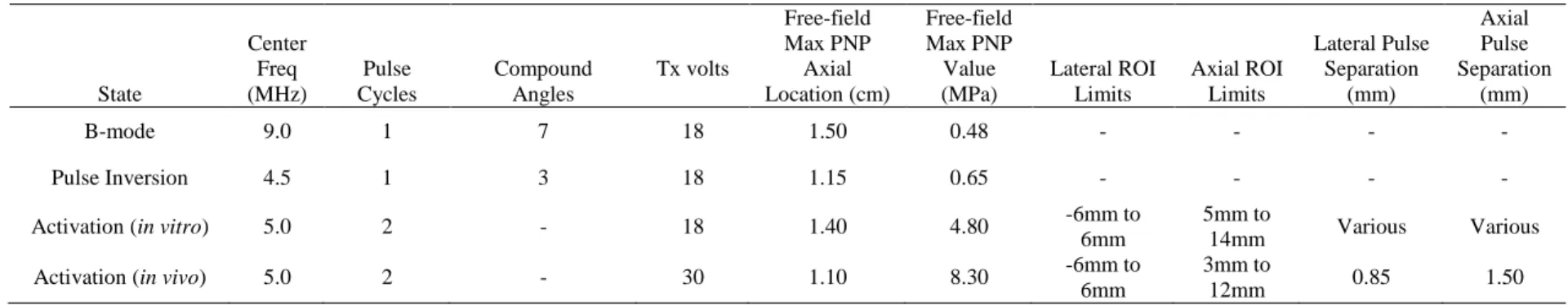
Table 4.1. Summary of imaging and activation design parameters. ... 66

Table 4.2. In vivo pressure estimations based on a simple tissue attenuation model. ... 87

Table 4.3. Vaporization Threshold for the different pulse lengths and dilutions. ... 98

Table 4.4. Vaporization Threshold used for comparing DFB and OFP. ... 101

(15)

xv

LIST OF FIGURES

Figure 1.1. Pulse inversion pulse sequence. ... 4

Figure 1.2. Amplitude modulation pulse sequence. ... 5

Figure 1.3. Cadence contrast pulse sequencing. ... 5

Figure 1.4. Example USMI protocol. B-mode is used for anatomical reference. ... 6

Figure 1.5. Time-intensity Curves for DCE-US. ... 8

Figure 1.6. Parametric perfusion maps overlaid on the corresponding B-mode images. ... 8

Figure 1.7. Overview of Acoustic Angiography. ... 10

Figure 2.1. Vaporization and expansion of low boiling-point PCCAs. ... 17

Figure 3.1. Summary of USMI imaging protocol. ... 24

Figure 3.2. Method for obtaining anechoic regions in a peak intensity image. ... 25

Figure 3.3. Example of individual response to the treatment. ... 26

Figure 3.4. Example USMI images of different treatment groups taken 7 min after injection. ... 32

Figure 3.5. Targeting intensity for the different treatment groups and timepoints. ... 33

Figure 3.6. Peak intensity for the different treatment groups and timepoints. ... 34

Figure 3.7. Percent Anechoic metric. ... 34

Figure 3.8. Tumor volume for the different treatment groups and timepoints. ... 36

Figure 3.9. Representative images of CD31 immunohistochemistry from USMI experiment. ... 37

Figure 3.10. Examples of individual responses of SU and Switch. ... 38

Figure 3.11. Representative perfusion maps overlaid on B-mode images for each treatment group. .. 40

Figure 3.12. Plots of volumetric perfusion times and tumor volume. ... 41

Figure 3.13. Representative maximum intensity projections of acoustic angiography images for the different treatment groups. ... 42

Figure 3.14. Results for the distance metric and sum of angles metric. ... 43

(16)

xvi

Figure 3.16. Tumor volume and blood vessel density for the different imaging weeks. ... 45

Figure 3.17. Plot of blood vessel density vs volume for all datapoints. ... 46

Figure 3.18. Representative CD31 staining images of the different treatment groups and Stained Area results. ... 47

Figure 3.19. Correlation plot of image derived blood vessel density vs CD31 stained neovasculature... 47

Figure 3.20. Linear regression model used to calcualate predicted tumor volume and ROC curve for predicted tumor volume as a classifier. ... 48

Figure 4.1.Imaging and activation sequence. ... 64

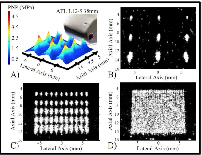
Figure 4.2. Transduer output pressure and activation clouds at different depths. ... 70

Figure 4.3. Example PWM pulse code and generated pulse. ... 72

Figure 4.4. Example APM parameters for in-vitro activation. ... 73

Figure 4.5. Pressure map with distance after accounting for attenuation using a rat kidney attenuation model. ... 75

Figure 4.6. Illustration of the analysis for the activation signal detection section. ... 78

Figure 4.7. Reconstruction technique for making VDI images. ... 79

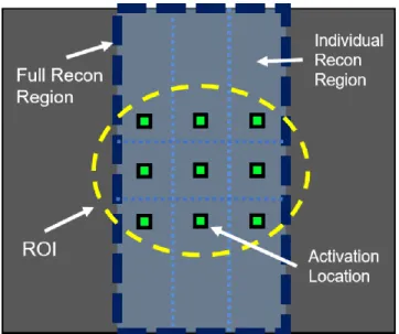
Figure 4.8. ROI drawn on b-mode image and activation locations. ... 80

Figure 4.9. Example CI image, and mask for analysis. ... 81

Figure 4.10. Representative distributions of contrast agents used in this study. ... 83

Figure 4.11. In vitro activation of DFB droplets. ... 84

Figure 4.12. Example overlays of B-mode ultrasound scans and contrast-specific pulse-inversion scans for each contrast agent tested. ... 88

Figure 4.13. Examples of contrast measurements taken for individual animals administered DFB and OFP droplets. ... 89

Figure 4.14. Maximum dB enhancement relative to the mean of the agent-free baseline for microbubbles after injection and droplets after application of a vaporization sequence. ... 90

Figure 4.15. Maximum contrast enhancement over the mean of the agent-free baseline normalized to the maximum value produced by each animal for microbubbles and droplets. ... 92

(17)

xvii

Figure 4.17. Intensity profiles were generated by averaging imaged data from activation lines separated by a range of distances between

0.25 and 1 mm. ... 94

Figure 4.18. APM and optimized spacing creates a region of uniform contrast. ... 95

Figure 4.19. OFP droplet activation in a rat kidney using APM and optimized spacing. ... 95

Figure 4.20. Contrast enhancement over the baseline case for each time point, and normalized to the one-minute time-point. ... 96

Figure 4.21. Example voltage traces from droplet vaporization detection. ... 97

Figure 4.22. AUC of tube signals after different filters. ... 98

Figure 4.23. AUC results of DFB and OFP for the different dilutions . ... 99

Figure 4.24. Mean Frequency results of DFB and OFP for the different dilutions. ... 100

Figure 4.25. AUC comparison between DFB and OFP for the different dilutions using the 25% threshold. ... 101

Figure 4.26. CE of in vivo data using different filters for both DFB and OFP. ... 102

Figure 4.27. Example in vivo VDI images from DFB and OFP.. ... 103

Figure 4.28. Example in vivo CI images of DFB and OFP before PCCA injection and at each activation pressure. ... 103

Figure 4.29. CE of VDI vs CI images for DFB and OFP. ... 104

Figure 4.30. CE of VDI and CI images of activation at depth in the 2 and 3 cm tubes before and after the introduction of droplets.. ... 104

Figure 4.31. CE of VDI and CI images from droplet activation in the microtubes at 2 and 3 cm. .... 105

Figure 5.1. Schematic of the pressurized chamber system used for part 2 of the in vitro experiments; testing the effect of hydrostatic pressure on droplet activation. ... 118

Figure 5.2. Example of activation scheme for US imaging measurement of activation in the 50 µm microtube and in a rat kidney. ... 122

Figure 5.3. Example fast Fourier transform of the received signal from the 1 MHz piston transducer. ... 123

Figure 5.4. Post-activation images of the different tubes and pressures. ... 124

(18)

xviii

Figure 5.6. Microscope images of droplet activation.. ... 126

Figure 5.7. Contrast enhancement generated by droplet activation inside the pressure chamber increased with peak-negative pressure under different hydrostatic pressures. ... 127

Figure 5.8. Contrast enhancement generated by droplet activation increased with pressure. ... 128

Figure 5.9. Example images of droplet vaporization in a rat kidney resulting from activation pulses of different pressures. ... 128

Figure 5.10. Example microscope image of droplet activation in 50 µm tube at 32X magnification. ... 130

Figure 5.11. AUC measurements from the 105 µm acrylic and 320 µm FEP tubes with a concentration of droplets matching the number of droplets in the 12.5 µm tube. ... 131

Figure 6.1. Summary of imaging protocol. ... 142

Figure 6.2. Summary of all experimental trials performed in each animal. ... 143

Figure 6.3. Illustration of the mask making process. ... 145

Figure 6.4. Example of data acquired by imaging protocol at the three different timepoints with example clearance curve and example wash-out curve with mean intensity data captured with CSS imaging after droplet vaporization. ... 145

Figure 6.5. Size distributions of MCAs and PCCAs using the Accusizer and NanoSight. ... 146

Figure 6.6. Example post-activation CSS, VDI, and MCA CSS images. ... 147

Figure 6.7. Targeting intensity for post-activation CSS and VDI at the different wait times. ... 148

Figure 6.8. Clearance rate

b

of control and targeted PCCAs. ... 148

Figure 6.9. Comparison of VDI and post-activation CSS for all wait times and doses. ... 149

Figure 6.10. Comparison of PCCAs and MCAs. ... 149

Figure 6.11. Targeting intenisty for the different wait times.. ... 150

Figure 6.12. Wash-out rate,

b

WO, for control and targetd PCCAs at all wait times. ... 151

Figure 6.13. Perfusion maps of MCA wash-in, control and targeted PCCA wash-out, overlaid over Bmode images. ... 155

(19)

xix

Figure 7.2. Size distributions for native and size-selected MCAs and the averaged wash-out curves for size-selected PCCAs. ... 166 Figure 7.3. Plots of wash-out rate and maximum contrast enhancement for different

size-selected OFP PCCAs doses and vaporization pressures. ... 167 Figure 7.4. Example microscopy image of vaporized PCCAs and plot of bubble

sizes for each number of cycles group. ... 168 Figure 7.5. Size distributions of size-selected DFB and OFB bubbles before

condensation and after vaporization for PEG2000 and PEG5000. ... 169 Figure 7.6. Example wash-out curves for size-selected OFP droplets with

C:18 and C:20 acyl chain lengths. ... 170 Figure 7.7 Wash-out rate and maximum contrast enhancement of vaporized

(20)

xx

LIST OF ABBREVIATIONS

AA Acoustic angiography

ADV Acoustic droplet vaporization ANOVA Analysis of variance

APM Activation pressure matching AUC Area under the curve

BVD Blood vessel density

ccRCC Clear-cell renal cell carcinoma CD31 Cluster of differentiation 31

CE Contrast enhancement

CEUS Contrast-enhanced ultrasound

CI Contrast imaging

CPS Cadence contrast pulse sequencing CSS Contrast-specific pulse sequence

CT Computed tomography

CTR Contrast-to-tissue ratio

DBPC 1,2-diarachidoyl-sn-glycero-3-phosphocholine DCE-US Dynamic contrast-enhanced ultrasound

DFB Decafluorobutane

DLL4 Delta-like ligand 4

DM Distance metric

(21)

xxi FEP Fluorinated Ethelyne Propylene

FOV Field of view

FSA Fibrosarcoma

GSI Gamma secretase inhibitor

HER2 Human epidermal growth factor receptor 2 MCA Microbubble contrast agent

MI Mechanical index

MRI Magnetic resonance imaging MTT Mean transit time

NSG NOD/scid/gamma

OFP Octafluoropropane

PA Percent anechoic

PBS Phosphate-buffered saline PCCA Phase-change contrast agent

PE Peak enhancement

PEG Polyethylene-glycol

PET Positron emission tomography

PFC Perfluorocarbon

PI Peak intensity

PNP Peak-negative pressure PWM Pulse-width modulation

RAD Cyclo-Arg-Ala-Asp-D-Tyr-Cys RCC Renal cell carcinoma

RECIST Response evaluation criteria in solid tumors RGD Cyclo-Arg-Gly-Asp-D-Tyr-Cys

(22)

xxii SOAM Sum of angles metric

STD Standard deviation

SU Sunitinib malate

TI Targeting intensity

US Ultrasound

USMI Ultrasound molecular imaging VDI Vaporization detection imaging VEGF Vascular endothelial growth factor VEGFR-2 Vascular endothelial growth factor 2

VHL Von Hippel-Lindau

(23)

1

CHAPTER 1 INTRODUCTION TO CONTRAST-ENHANCED ULTRASOUND

1.1 Motivation

Cancer is the second leading cause of death in the United States behind cardiovascular disease, and will claim the lives of over 600,000 Americans in the coming year [1]. Because of the lethality of the disease, proper staging and accurate assessment of response to different therapies is critical to optimize therapy and correctly assess prognosis. Assessing the initial response is important for survival outcome, but tumors can develop resistance to different therapeutic regimens and show progression even if the disease seems to be controlled initially [2,3]. Therefore, it is equally important to accurately track the progression of the disease throughout treatment in order to better tailor therapy and enhance efficacy. For example, it has been shown that resistance to therapy can cause a rebound effect where the tumor becomes more aggressive, and this rebound can be worse in cases that showed a better initial response [2]. As such, it is very important to closely track the disease to provide effective treatments and avoid harmful outcomes.

1.2 Limitations of Current Clinical Diagnostic Techniques

(24)

2

therapies such as radio and chemotherapies that directly kill cancer cells but not for therapies such as antiangiogenic drugs that attack the tumor vasculature [3,12]. These therapies often do not cause tumor shrinkage and are thus incorrectly categorized using tumor size criteria [13,14]. Studies have found that RECIST severely underestimated the response of antiangiogenic therapies in renal cell carcinoma (RCC) and could identify progression-free survival in less than 20% of patients [3,12].

1.3 Biomedical Imaging for Assessment of Response to Therapy

(25)

3

cause nephrogenic systemic fibrosis (fibrosis in skin and lungs and then heart, liver, kidneys) for patients with advanced chronic kidney disease, which can lead to death [24,25].

1.4 Contrast-Enhanced Ultrasound and Microbubble Contrast Agents

In comparison to the imaging modalities discussed in the previous section, contrast-enhanced ultrasound (CEUS) imaging is inexpensive, portable for bed-side diagnostics, widely available, and does not involve any ionizing radiation. CEUS uses contrast agents that are safe for clinical use [26,27], range in size between 1 and 5 µm and thus can freely traverse the vasculature, and have been used for molecular and perfusion imaging of disease [28–31]. Therefore, CEUS can be a powerful tool for serial monitoring of disease and assessment of early response to therapy. Conventional microbubble contrast agents (MCAs) are typically composed of a phospholipid shell to prevent dissolution and coalescence [32] and have cores with gases, such as sulfur hexafluoride or perfluorocarbons (PFCs), which have high molecular weight and low solubility in blood to decrease dissolution and enhance circulation time. Adding polyethylene glycol (PEG) to the shell of nanoparticles has been common practice for decades in the field of drug delivery, as PEG provides a steric shield that prevents immune cell recognition and dramatically decreases particle clearance by the mononuclear phagocytic system, also known as the reticuloendothelial system [33–35]. Hence, PEG is commonly conjugated to the lipid shell to reduce MCA coalescence and recognition by the immune system [36,37] and to attach targeting ligands for molecular imaging [38,39].

(26)

4

1.5 Pulse Sequences for Contrast-Enhanced Ultrasound

Contrast-specific sequences separate MCA signals from tissue signals based on their non-linear frequency and amplitude response. Specifically, tissue response to transmitted ultrasound waves is predominantly linear, producing echoes having a frequency content dominated by the excitation frequency and an amplitude linearly proportional to that of the incident pressure wave. Conversely, the frequency content of signals produced by MCAs encompasses the excitation frequency as well as significant energy at higher harmonics [40], and the resulting signal amplitude is not linearly proportional to the excitation pressure [41]. Techniques such as pulse inversion [42] (Figure 1.1) and amplitude modulation [41] (Figure 1.2) take advantage of the non-linear response of MCAs to reduce tissue signal and produce images with a high contrast-to-tissue ratio (CTR). CadenceTM_{contrast pulse} sequencing (CPS) from Siemens Medical Solutions, Inc. (Issaquah, WA, USA) incorporates pulse inversion and amplitude modulation to produce an US sequence that reduces tissue signal and is more sensitive to MCA signal than either pulse inversion or amplitude modulation alone [43] (Figure 1.3).

(27)

5

Figure 1.2. Amplitude modulation pulse sequence. This approach consists of subtracting twice a half-amplitude pulse from a full-half-amplitude pulse to eliminate fundamental tissue signals.

Figure 1.3. Cadence contrast pulse sequencing. Pulse inversion and amplitude modulation are combined to eliminate tissue signal and isolate fundamental and second harmonic frequency components from MCAs. A full-amplitude pulse is followed by 2 inverted and half-amplitude pulses.

1.6 Ultrasound Molecular Imaging

(28)

6

cardiovascular disease [44–46], inflammatory disorders [47,48], and angiogenesis [49–51]. Typically, biomarkers expressed on the vascular endothelium such as αvβ3 integrin and the Vascular Endothelial Growth Factor receptor (VEGFR-2) are targeted [49,52–55] because available markers are partially limited by the confinement of the microbubbles to the microvasculature due to their size.

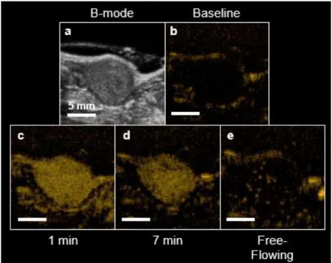
Figure 1.4. Example USMI protocol. B-mode is used for anatomical reference (a). Contrast-specific sequences greatly reduce the tissue signal (b). MCAs are injected and perfuse the entire tissue (c). MCAs are allowed to bind for several minutes while freely-flowing agents are cleared from circulation (d). A destructive flash clears bound MCA from the tumor, so that the level of freely-flowing signal can be captured (e). The USMI signal is calculated by subtracting (e) from (d).

(29)

7

the two scans [49] (Figure 1.4). This approach reduces the imaging time because it is not needed to wait until all of the freely-flowing MCAs have been cleared from circulation by the liver and lungs.

1.7 Dynamic Contrast-Enhanced Ultrasound

Since MCAs are constrained to the vasculature, CEUS can image characteristics of blood such as perfusion rate, by monitoring the transit time of MCAs leaving or arriving into a target or measuring how long they remain in the tissue. Dynamic contrast-enhanced ultrasound (DCE-US) can produce a quantitative measurement of perfusion that can be used to evaluate functional changes, something that is difficult to do with other US techniques such as Doppler. DCE-US has been shown to measure tissue characteristics such as blood perfusion [56–58] for cardiology [59,60], evaluation and treatment of ischemic stroke [61–63], and cancer assessment and management [64,65] in animal models of disease.

(30)

8

Additionally, the time for the intensity inside the ROI to reach 20% (20% is common, but any percentage can be used) of the value before the destructive flash can be used as a metric of perfusion.

Figure 1.5. Time-intensity Curves for DCE-US. A bolus of MCAs is introduced and the signal is monitored until the agents are cleared from circulation (left). Perfusion metrics such as mean transit time (MTT), peak enhancement (PE), and area under the curve (AUC) can be calculated. The Destruction Reperfusion protocol (right) involves measuring the intensity after a destructive flash clears MCAs from the field of view. A perfusion coefficient α and a time to 20% of baseline can be calculated to quantify perfusion.

Using a similar protocol to Destruction Reperfusion, the same perfusion metrics can be calculated for each pixel in the image to create parametric perfusion maps that allow for quantification of specific areas in the ROI [56,58,68] (Figure 1.6).

(31)

9

1.8 Acoustic Angiography

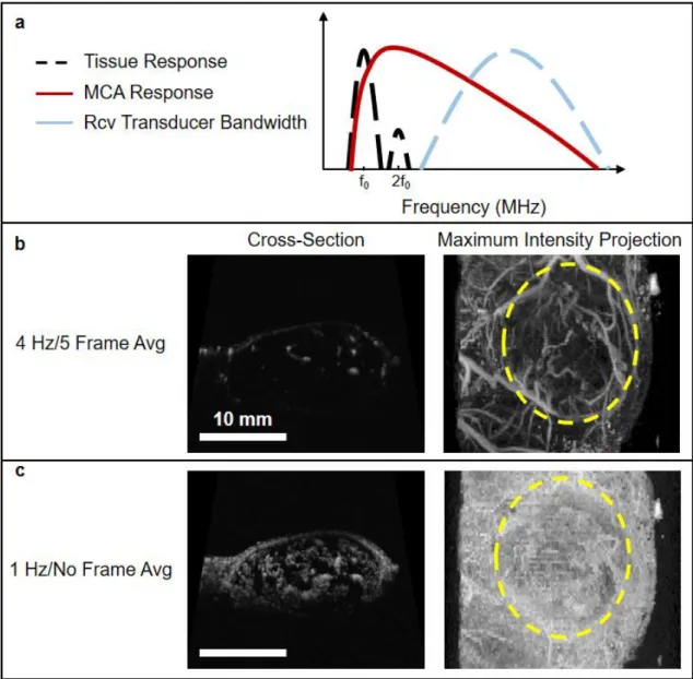
Acoustic angiography (AA) is another CEUS technique which uses the super-harmonic signals from MCAs to produce high resolution maps of vasculature [40,69]. Specifically, tissue response to transmitted ultrasound waves is predominately linear, producing echoes having the same frequency content dominated by the excitation frequency. Conversely, the frequency content of signals produced by MCAs encompasses the excitation frequency as well as significant energy at higher harmonics [40]. The potential of superharmonic imaging was first demonstrated by Bouakaz et al. [70] and Kruse and Ferrara [71], where it was observed that broadband energy exceeding 45MHz was produced when microbubbles were excited with short 2.5 MHz pulses. Therefore, AA consists of exciting microbubbles at their resonant frequency (typically less than 10 MHz), and receiving at a high frequency (10-30 MHz) to capture their higher harmonic content response, and thus eliminating the fundamental frequency content of tissue (Figure 1.7a). The microbubble harmonics can be detected at several fold of the fundamental frequency, resulting in images with substantially higher resolution and higher CTR than obtained with existing technology [69].

(32)

10

“cloudy” images containing MCA signal from both sub-resolution and resolvable vessels (Figure 1.7c) that can provide a quantitative measure of microvascular density [74]. Furthermore, a measure of perfusion can be obtained by adjusting imaging parameters, since the main difference between the two types of AA images discussed above is the length of time allowed for re-perfusion between frames [75].

(33)

11

Cancer is characterized by extensive angiogenesis, or the formation of new vasculature [76]. As tumors grow, they use different signaling pathways such as the vascular endothelial growth factor (VEGF) and Notch signaling pathways to recruit new vasculature and feed the rapidly growing number of cells [76,77]. However, angiogenesis in cancer is different than that of normal physiological processes, in that it results in abnormal vasculature that is often disorganized and tortuous due to an excess in signaling [78]. It has been shown that vascular remodeling in cancer can start when the tumor is as small as 100 cells [79], and morphological changes in the vasculature can be detected using AA before the tumor is palpable, or around 2-3 mm [72]. Therefore, AA might be an ideal technique for tracking and assessing the response of cancer to different therapies.

1.9 Overview of Pre-Clinical CEUS for the Assessment of Response to Therapy

Over recent years, researchers have started exploring the potential of CEUS to assess the response of disease to different therapies in rodents. Within the last 3 years, many studies have demonstrated the ability of USMI to target VEGFR-2 in different cancer models and provide imaging results that correlate with histology [80–85]. In line with these findings, some studies have shown that USMI of VEGFR-2 can be used to predict response to antiangiogenic therapy earlier than tumor volume [81–83]. Furthermore, Wang et. al showed that the effects of antiangiogenic therapy can be observed with USMI and DCE-US as early as 24 h after treatment [86]. Streeter et al. found that USMI of αvβ3 integrin is capable of differentiating between patient-derived xenografts that respond to aurora-A kinase inhibition and non-responders earlier than tumor volume as an indicator [87], and Sirsi et al. demonstrated that USMI can predict response of antiangiogenic therapy earlier than volume measurements [88].

(34)

12

vascular density from AA to differentiate between responders and non-responders in tumors treated with radiation [74].

It is worth noting that there have been a handful of clinical studies that use DCE-US to assess early response to antiangiogenic therapy in renal, hepatic, and gastrointestinal cancers [20,90–93] and have shown promising results. However, even though targeted agents for USMI have recently been approved for patient use, there are not studies, to my knowledge, that have used USMI for the assessment of response to therapy in human patients.

(35)

13

CHAPTER 2 PHASE-CHANGE CONTRAST AGENTS

2.1 Introduction to Phase-Change Contrast Agents

Phase-change contrast agents (PCCAs) were introduced almost two decades ago for therapeutic applications, such as occlusion therapy [94–96], cavitation enhancement for tumor ablation [97–100], and aberration correction for diagnosis [94,101,102]. PCCAs conventionally have liquid cores composed of a perfluorocarbon (PFC) with a boiling point around body temperature, which can be vaporized, or activated, into microbubbles using ultrasound in an event termed acoustic droplet vaporization (ADV) by Kripfgans et. al [101]. ADV has been studied extensively over the years [103– 110], and it has been found that acoustic vaporization of the liquid core is initiated by superharmonic focusing; high frequencies that can have wavelengths around the size of the agent are created by non-linear propagation and focused because of the difference in speed of sound between the PFC core and media around the agent [109,111]. Because ADV produces bubbles many times the size of the precursor PCCAs, these agents could be used in the occlusion of vessels for starving cancerous tissue or providing point targets for aberration correction.

2.2 PCCAs for Therapy

(36)

14

offsite effects are common due to the high acoustic pressures used [115]. Using MCAs allows localization of the therapeutic effect to the target by providing cavitation nuclei but can cause skin lesions when the concentration of agents is too high [116]. Since PCCAs require acoustic pressures that exceed a certain threshold to become microbubbles, cavitation will only occur around the focus of the US pulse where that threshold is achieved, which helps to precisely control the location of the treatment [98–100]. Furthermore, PCCAs have been used for MR-guided tumor ablation [117,118], and cavitation of microbubbles created by ADV has been used for sonoporation in cells [119].

PCCAs can be manufactured to have a size of 100-400 nm, which may allow them to escape the vasculature in cancerous regions which have disorganized and “leaky” endothelial structures that allow nanoparticle diffusion into the tissue [120–122]. As such, PCCAs can be loaded with drugs and allowed to extravasate and accumulate in the tumor tissue for highly localized delivery [123–125].

2.3 PCCAs for Diagnosis

Although used mainly for therapy, PCCAs have characteristics that can overcome limitations associated with microbubble contrast agents, namely, short circulation time in vivo and the inability to extravasate, due to their size, to provide contrast for diagnosis or deliver therapeutic agents into the interstitium. Furthermore, the liquid core greatly reduces dissolution of the PFC into the blood and expiration through the lungs. Because of these advantages and the fact that PCCAs can be vaporized to form echogenic microbubbles capable of providing contrast, droplets have great potential for diagnostic applications, such as molecular and perfusion imaging [126,127].

2.4 Stability of PCCAs at Room and Body Temperature

(37)

15

precipitates nucleation of vapor embryos and subsequent vaporization of the entire droplet [107,108,130,131,133]. However, PCCAs have historically been composed of PFCs that are liquid at room or body temperature, such as perfluorpentane or perfluorohexane. Vaporization of these “liquid” PFCs in nano-sized PCCAs requires more energy than micron-sized droplets, so the high acoustic pressures required for activation exceed the Food and Drug Administration limit for diagnostic imaging.

2.5 Low Boiling-Point PCCAs

High boiling-point PCCAs may be desired for therapeutic applications because of enhanced stability in vivo and resistance against spontaneous vaporization. Additionally, their stability allows for spatial and temporal control of activation, since vaporization occurs only in areas targeted by acoustic energy and once a high acoustic pressure threshold is achieved. However, there has also been an interest in PCCAs that can be vaporized at low acoustic pressures well within the diagnostic ultrasound regime. Sheeran et al. developed sub-micron PCCAs using low-boiling PFCs that are stable at body temperature and can be vaporized using imaging acoustic pressures [128,129,134]. These low-boiling point droplets are typically composed of either decafluorobutane (DFB, -2ºC boiling-point), octafluoropropane (OFP, -37ºC boiling-point), or mixtures of these perfluorocarbons. Mixing the PFCs allows for tailoring of the vaporization threshold, so low boiling-point PCCAs have been used in vitro as temperature probes [135].

(38)

16

can be activated using short pulses (< 10 cycles) like those found in clinical scanners, using diagnostically relevant pressures, and that the microbubbles resulting from ADV have sizes similar to those of conventional MCAs or the precursor microbubbles that were condensed to make the PCCAs [130,134]. It is worth noting, however, that the resulting microbubble size after vaporization is often larger than the precursor bubble due to gasses in the environment diffusing in for several seconds after activation [128]. It has been observed that the lipid shell is conserved after condensation [134] and vaporization [136] by fluorescently labelling the shell, so it is not clear why the resulting microbubble is more permeable to gases in the environment. Furthermore, targeting ligands can be attached to the lipid shell since it is retained through condensation and vaporization, and molecular imaging has been demonstrated in vitro [126].

2.6 Vaporization Signal of Low Boiling-Point PCCAs

In addition to producing highly echogenic microbubbles, the vaporization event of low-boiling point PCCAs produces very specific acoustic signatures [137]. As the droplet is vaporized, it over-expands and oscillates down to its final size, producing acoustic signals between 0.25 and 2.5 MHz regardless of the excitation frequency (Figure 2.1). Furthermore, the vaporization signals have large amplitudes compared to those resulting from exciting microbubbles with the same pressures, and so, isolating droplet activation signatures may produce images that are specific to PCCAs and eliminate tissue or microbubble signal. Moreover, the low frequency of activation signals may provide better depth of penetration than conventional contrast ultrasound.

(39)

17

Figure 2.1. Vaporization and expansion of low boiling-point PCCAs. The agent overexpands and oscillates down to its final diameter. The resulting bubbles are around 5 times larger than the PCCAs.

In addition to the work mentioned previously, there have been in vitro studies on the condensation of PCCAs [140], the stability of the bubbles produced by PCCA vaporization [104,141], the effect of channel confinement on the contrast provided by PCCA activation [142], and characterization of vaporization using frequencies above 20 MHz [143], but few studies outside the work presented in this thesis have used PCCAs, either high or low-boiling point, for in vivo diagnostic imaging [143–145]. It is worth noting that in one of these studies, Nyankima et. al demonstrated that low boiling-point PCCAs can be safely used in vivo without causing bioeffects [145].

2.7 Possible Advantages of PCCAs for Diagnostic Imaging

(40)

18

be detected, instead of changes in markers such as VEGFR-2 that are general to all cancers. For example, increased expression of human epidermal growth factor receptor 2 (HER2) in 25% to 30% of breast cancers correlates with poor disease-free and overall survival [146,147]. Additionally, anti-HER2 antibodies such as trastuzumab have been shown to have significant anti-tumor capabilities and to enhance the efficacy of treatment when used in conjunction with chemotherapy but only in tumors overexpressing HER2 [146,148,149]. Therefore, imaging HER2 can be important to identify aggressive breast cancers with overexpression of HER2 that may not respond well to chemotherapy and to determine if drugs, such as trastuzumab, are viable treatment options.

PCCAs may extravasate due to the enhanced permeability and retention (EPR) effect [120] and bind to markers expressed by cancer cells. In theory, the unbound PCCAs would then be cleared by the lymphatic system, leaving only bound droplets which could be vaporized to obtain USMI signal.

(41)

19

CHAPTER 3 ASSESSMENT OF TUMOR RESPONSE TO THERAPY USING MICROBUBBLE

CONTRAST AGENTS

1,2

3.1 Introduction

In this chapter, the ability of CEUS to assess tumor response to therapy is demonstrated. The chosen model is a clear-cell renal cell carcinoma (ccRCC) xenograft that was evaluated using USMI, DCE-US, and AA.

Metastatic clear-cell renal cell carcinoma results in over 14,000 deaths annually in the US, and over 60,000 new cases are expected to be diagnosed this year [1]. This type of cancer is characterized by increased angiogenesis due to gene mutations in the von Hippel-Lindau gene (VHL), which upregulates various pro-angiogenic factors [150,151]. A common clinical therapeutic strategy for the treatment of ccRCC is antiangiogenic treatment [9,152–155]. Drugs such as Sunitinib, a small molecule multi-kinase inhibitor, reduces the signaling of the vascular endothelial growth factor (VEGF) pathway via its receptor VEGFR-2 [9,152–155]. The VEGF pathway plays a key role in tumor angiogenesis, such that inhibition reduces new vessel formation and starves the tumor. Antiangiogenic therapy is initially effective against ccRCC, which is characterized by increased angiogenesis [150,151], although

Chong, VL Bautch, WK Rathmell, PA Dayton, “Ultrasound Molecular Imaging of VEGFRR-2 in Clear-Cell Renal Cell Carcinoma Tracks Disease Response to Antiangiogenic and Notch-Inhibition Therpy”, Theranostics, 2018; 8(1): 141-155.

(42)

20

resistance to anti-angiogenic therapy is almost universally developed after several months of therapy [156–158].

Inhibition of the Notch signaling pathway is an alternative strategy to antiangiogenic therapy that also impairs angiogenesis. Notch signaling promotes vessel growth while suppressing excessive sprouting by down regulating VEGFR-2 on endothelial cells of the growing stalk [159–161]. Endothelial tip cells induce adjacent stalk cells to pattern new vessels [160–162]. Binding between Notch ligands such as Dll4 (Delta-like ligand 4) on tip cells and Notch receptors on stalk cells regulates the specialization of endothelial cells and limits sprout numbers [160,161]. This signaling pathway can be inhibited using gamma secretase inhibitors, which inhibit the activation of Notch via cleavage induced by ligand binding. Therefore, inhibiting Notch signaling yields a disproportionate number of tip cells, resulting in excessive sprouting and immature vasculature, which has been shown to inhibit tumor growth, likely due to inefficient perfusion [160,163–166]. These complementing inhibitory pathways provide an opportunity for parallel angiogenic blockade, and moreover, the additional expression of VEGFR-2 caused by the inhibition of Notch might cause ccRCC undergoing Notch inhibition to re-sensitize to the effects of VEGF receptor targeting. This proposed interaction has the potential to be a mechanism for overcoming resistance to conventional antiangiogenic therapy in ways that may be challenging to monitor with conventional imaging.

(43)

21

vasculature. Furthermore, since Notch inhibition produces excess sprouting, the enhanced tortuosity might be captured using AA and could be a good indicator of response.

3.2 Methods

3.2.1 Microbubble Contrast Agents

The contrast agents used for the USMI part of the study were VEGFR-2 targeted perfluorocarbon microbubbles (Visistar VEFGR2, Targeson, San Diego, CA, USA) with a mean diameter of 2.23 ± 0.02 μm. Competitive binding experiments show that Targeson VEGFR-2 bubbles produce significantly higher retention in tumors than similar control bubbles bearing isotype-matched antibodies [49], inactivated antibodies [167], or naked microbubbles without targeting antibodies [168].

The lipid-encapsulated perfluorocarbon MCAs used in the rest of this work were manufactured in-house and were similar to commercial lipid-shelled contrast agents. The lipids 1,2-distearoyl-sn-glycero-3-phosphocholine and 1,2-distearoyl-sn-glycero-3-phosphoethanolamine-N-methoxy (polyethylene-glycol)-2000 (DSPE-PEG2000) in a 9:1 M ratio and a total lipid concentration of 1.0 mg/mL were dissolved in a solution of phosphate-buffered saline, propylene glycol, and glycerol (16:3:1). Then, 1.5 mL of the solution was added to a 3-mL glass vial and the head space was gas-exchanged with decafluorobutane gas. Microbubbles (1 µm mean diameter and a 1x1010 _#/mL concentration) were produced by using an agitation technique.

3.2.2 Xenograft and Treatment Protocol

(44)

22

Treatment started when the tumors reached 200 mm3_{(caliper measurement) and continued for} 5 weeks. The drugs used were a Notch pathway inhibitor GSI (Gamma secretase inhibitor, PF-03084014, Pfizer, New York, NY, USA) at a daily dose of 90 mg/kg, and VEGF inhibitor SU (Sunitinib malate, Selleckchem, TX, USA) at a daily dose of 50 mg/kg. The therapies were delivered by oral gavage.

For the USMI experiment a total of 32 mice were placed into 4 treatment groups: GSI, SU, a Switch group (SU to GSI), and Control (100 µL of saline). In the case of the Switch group, the mice were treated with SU for 3 weeks before switching to GSI.

For the DCE-US portion of this work, the mice were treated daily with GSI, SU, a combination of the two drugs, or saline. There were 4 mice per group, except for the GSI group, which had 3 animals.

The AA experiment contained 2 sections: vascular morphology (tortuosity) and vascular density analysis. For the morphology portion, 9 mice were divided into 3 groups: GSI, a combination of GSI and SU, and a Control (saline). The number of animals in each group for the density experiment were 8, 16, and 8 for the Control, SU, and Combo groups, respectively.

3.2.3 Animal Protocol and Contrast Administration

(45)

23

For the USMI experiment, a bolus of 2x106_{of the Targeson microbubbles diluted in 100 µL} of sterile saline was injected, followed by a 100 µL saline flush to clear the catheter and ensure the entire dose was delivered. An Accusizer 780 A (Particle Sizing Systems, Santa Barbara, CA, USA) was used to size the bubbles before every imaging session to ensure a precise dose was injected for all experiments. In-house MCAs were continuously infused at a rate of 6x107_{bubbles/min for the} DCE-US portion, and at a rate of 1.5x108_{bubbles/min for both sections of the AA experiment.}

3.2.4 Imaging and Analysis Protocols

3.2.4.1 USMI

(46)

24

Figure 3.1. Summary of USMI imaging protocol. A baseline contrast scan was captured prior to the microbubble injection (A). A scan to capture the maximum peak intensity was taken 1 min after the introduction of contrast (B). The bubbles were allowed to circulate and bind for 7 min, at which time a contrast scan was taken (C). Destructive pulses clear the tumor of both bound and freely-flowing bubbles (D), and the level of freely-flowing contrast was obtained 1 min after destruction to allow bubbles to reperfuse the tissue (E). Note: data was only collected at B, C, and E and the solid black line is only an estimate of the intensity over time.

(47)

25

microbubbles spread throughout the body and circulate the vasculature several times in one minute and therefore, anechoic regions that have not been perfused by that time do not have patent vasculature and should be excluded from analysis. Since our intent is to compare biomarker presence within the vasculature, inclusion of regions without perfusion would bias this result.

Anechoic regions appear dark in the contrast images, but due to the nature of speckle, an area that is completely perfused will also contain small dark regions. Eliminating pixels that have intensities lower than a certain threshold would thus eliminate regions that are perfused in addition to regions that are anechoic. Therefore, the images were blurred using a Gaussian filter in order to eliminate small dark regions in areas that are full of contrast, in essence eliminating the speckle (Figure 3.2). Next, the regions of the image that were inside the analysis ROI and had an intensity lower than a predefined threshold were removed from the analysis region for the calculation of all metrics. The threshold was defined using preliminary data, and the same value was used for all animals at every time point. Furthermore, the different treatments affect functional characteristics of the tumor, such as perfusion, so the volume of the anechoic areas was used to calculate a “percent anechoic” (PA) metric to assess the response of the disease to the treatment over time. This metric is related to the amount of patent vasculature in the tumor volume, or lack thereof, due to necrosis or other factors.

Figure 3.2. Method for obtaining anechoic regions in a peak intensity image (A). The green dots outline the tumor. The image is blurred using a Gaussian filter to eliminate dark areas in speckle (B). The regions below a predetermined intensity threshold are selected as anechoic (C). Note: these are single frames in a 3D volume, so the process will be performed for each slice in the volume.

(48)

26

above (or below) the threshold for individual mice at the different time points represented response to the treatment. For example, the individual volume (solid black line) in Figure 3.3 becomes smaller than the volume threshold (dashed black line) 3 weeks after the start of treatment, so it can be said that response was detected in the tumor volume at this time. The threshold value at each time point was calculated as the first quadrant of the grouped Control data at each time point for the TI and volume and the third quadrant for the PA. Finally, the percentage of mice in the SU and Switch groups that showed response (sensitivity) to the therapy using each metric was calculated for the first 3 weeks of treatment. The process was repeated for the control mice using the same threshold as with the treated mice to find percentage of animals that were correctly identified as untreated (specificity).

Figure 3.3. Example of individual response to the treatment. The solid lines represent either the TI (dark gray), PA (light gray), and the volume (black) for a single animal, while the dashed lines represent the threshold for each metric calculated using the Control group data. Each metric was determined to show resistance if the individual value (solid) was lower, for the TI and Volume, or higher, for the PA, than its threshold (dashed). The data for each metric were normalized to the pretreatment value, and by an additional factor in order to display the curves in the same scale.

3.2.4.2 DCE-US

(49)

27

capture the reperfusion of bubbles back into the FOV. It has been shown that blood flow characteristics can be very heterogeneous in tumors [58], so the imaging sequence was repeated for five different cross-sections to capture the 3D perfusion of the tumor by scanning the transducer in the elevation direction using a computer-controlled motion stage [58]. Since the number of imaging cross-sections was set to five for all experiments, the spacing between imaging locations varied depending on the size of the tumor. A maximum of five planes were imaged because of infusion volume limitations.

For each imaging plane, a parametric perfusion map was generated by calculating the amount of time it took each pixel to reach 80% of the mean intensity from its baseline CPS frames, which is similar to what has been previously reported [56,58]. Pixels that did not reach the threshold in 40 s were left blank and will be referred to as anechoic areas. The mean value of the area inside the ROI of each perfusion map was calculated and averaged to obtain a volumetric perfusion time (VPT) for the entire tumor. The tumor volume was calculated by multiplying the total number of voxels inside the 3D ROI by the size of the voxels.

3.2.4.3 AA- Morphology

To acquire AA images, a Vevo 770 ultrasound system (VisualSonics, Toronto, Canada) was used to control a prototype transducer that allows for transmission at 4 MHz and reception of MCA super harmonic signals around 30 MHz [171]. Two co-aligned, single-elements were mechanically swept and one element was used only for transmit and the other only for receive. The low-frequency element was excited with a single-cycle sinusoid and produced a signal with a peak-negative pressure of 1.2 MPa [72]. In order to explore the changes in morphology resulting from the different therapies, a frame rate of 4 Hz with 5-frame averaging was used to isolate resolvable vessels and eliminate sub-resolution information, as was explained in Chapter 1. Additionally, the transducer was translated elevationally in steps of 100 µm to acquire 3D vascular images.

(50)

28

the tortuosity, or “bendiness”, of the vessels was computed using different metrics previously described by Bullitt et al. [173], and used to characterize tumor vasculature from AA [40,72]. The metrics used were the distance metric (DM) and the sum of angles metric (SOAM). The DM was computed by dividing the length of the vessel by the Euclidian distance between start and end points, and the SOAM is found by calculating the integral of the curvature and normalizing by the vessel length, where the curvature is found by adding the angles between successive groups of 3 points along the vessel. While the DM is appropriate for vessels that loop or arc, the SOAM is effective for vessels that have high-frequency changes in curvature over short distances. Both types of vessels are found in tumors, but it has been found that the SOAM is a better metric for quantifying the tortuosity of cancer vasculature and separating between tumor and normal vessels [40,72]. Nevertheless, both metrics were used to evaluate the response of the tumors to the different therapies.

3.2.4.4 AA- Vascular Density

The imaging system used for this section was a VegaTM_{platform (SonoVol, Inc., Research} Triangle Park, NC), which allows for automated 3D ultrasound image acquisition from mice. The system was used in both high-frequency/high-resolution B-mode for anatomical reference and AA mode for microvascular analysis.

A 3D B-mode “scout scan” with an elevational resolution of 200 µm of was used to locate the tumor. Next, AA images were captured around the tumor location 30 seconds after the start of the MCA infusion. AA imaging consisted of a continuous sweep acquisition, which produced images of vasculature with an elevational resolution of around 500 µm. The tumor was scanned 16 times, allowing MCAs to reperfuse into the tissue for 10 seconds between each scan, and a final AA image was computed by averaging all the acquisitions.

(51)

29

microvasculature images by dividing the number of voxels with intensity values higher than a fixed, predetermined threshold by the total number of voxels in the ROI. The tumor volume was calculated by summing the number of voxels inside the ROI and multiplying by the spatial dimensions of a voxel.

For calculating the BVD, a threshold that separates MCA signal from noise was first found. The threshold selected for all time-points was the value that provided the highest correlation coefficient (ρ) between the imaging results from the last imaging time-point and the results from histological analysis (described in the following section). The correlation coefficient was calculated using a right-tailed Spearman test and was used to evaluate how well the BVD results from imaging correspond to real physiologic characteristics of the tissue.

3.2.5 CD31 Immunohistochemistry

CD31 immunohistochemistry was performed to serve as a gold standard for comparison against imaging results. Tumors were harvested after the last imaging time point or earlier if the size limit was exceeded, or due to poor health. Three tumors from each treatment group of the USMI and vascular density experiments were used for the histological analysis, except for the SU group in the vascular density portion, from which 6 tumors were used. Immunohistochemistry was performed on paraffin-embedded tumor sections on a Leica Bond Max autostainer using anti-CD31 from Novocastra (cat # NCL-CD31-1A10). Following heat-induced epitope retrieval in EDTA for 20 min, the antibody was incubated on the tissue for 1 h at a dilution of 1:100 then visualized with diaminobenzidine (DAB). Thirty stained sections from each treatment group were captured by an Olympus DP 72 or an Infinity2 camera at 200x, and the percentage of positively stained area was determined using NIH ImageJ [174]. A separate cohort of animals was treated with SU and their tumors were harvested after 3 weeks of treatment to obtain a pre-switch measurement of patent vasculature for the USMI experiment.

3.2.6 Statistical Analysis

(52)

30

significance between each of the groups. Statistical analysis was performed on all mice available at each time point, regardless of whether the animal survived through the end of the study. ANOVA analysis was used to find any significance between the groups for histology and vessel morphology instead of the Kruskal-Wallis method. Significance was set at p < 0.05.

A right-tailed Spearman test was used to assess the correlation between the last imaging BVD timepoint (vascular density analysis section) and histology for different threshold values in order to select the most appropriate threshold.

Furthermore, the BVD at early time points was used to predict response to treatment (treated vs untreated, inferred from the tumor volume at later time points). The BVD around day 7 (day 6 to 10) after the start of treatment was plotted against the corresponding tumor volume measurements from around day 21 (day 17 to 24). A linear regression model was used to fit the data, so that a predicted tumor volume (PTV) for each animal could be calculated from the BVD around day 7. Next, PTV values above and below a threshold were classified as untreated or treated, respectively, for a range of thresholds. Using receiver-operator curve (ROC) analysis, the PTV threshold that produced the best sensitivity (true positive) and specificity (true negative) at separating treated and untreated was calculated.

3.2.7 Organization of Data

(53)

31

3.3 Results

3.3.1 USMI

(54)

32

(55)

33

A significant difference in targeting intensity (TI), a measure of VEGFR-2 expression, can be seen 2 weeks following the start of treatment (Figure 3.5). TI for SU became, and remained, significantly lower than that of the Control group after the first week (p < 0.05 for all time points after the first week of treatment), while the TI of the GSI group remained non-significant from the Control group for the duration of the experiment. TI for the Switch group mimicked that of the SU group for the first 3 weeks after the start of treatment, but it increased after the switch to GSI and became non-significant from the GSI and Control groups 1 week after the switch. It is important to note that when the SU and Switch groups are combined, the TI was significant (p < 0.05) from that of the Control group 1 week after the start of treatment. Additionally, a subset of the SU and Switch groups was imaged 2 days after the start of treatment and there was a significant difference (p < 0.05) in the TI between this early time point and the baseline scan. USMI was able to closely track changes of VEGFR-2 expression as the result of the two types of therapy.

(56)

34

Figure 3.6. Peak intensity (PI) for the different treatment groups and timepoints. PI was typically lower for the groups treated with SU but this relationship was only significant 3 weeks after the start of treatment. PI increased for the Switch group once the mice were treated with GSI and became significant from SU 2 weeks after the switch.

(57)

35

The peak intensity signal (PI), captured 1 min after the injection of contrast, was reduced for the SU and Switch groups in comparison to the Control and GSI groups, but the results were only statistically significant (p < 0.05) 3 weeks after the start of treatment (Figure 3.6). The Switch group PI became significant from that of the SU group 5 weeks after the start of treatment. The PI did not provide any significant trends or differences between groups that indicate the ability to track response to therapy.

The groups that were treated with SU showed increased percentages of anechoic regions (PA) as the treatment progressed (Figure 3.7). The SU and Switch group became significantly higher (p < 0.05) than the Control 2 weeks after the start of treatment and 1 week after the start of treatment compared to the GSI group. The SU group remained significantly higher than the Control and GSI groups for the remainder of the study, except on the last time point, while the Switch group decreased after the switch to GSI and became non-significant from the Control and GSI groups and significant from the SU group (p < 0.05) the week following the switch. The PA for the GSI and Control groups steadily rose throughout the study but remained smaller and non-significant from the SU group. PA provided a useful measure of how the therapy was affecting the amount of patent microvasculature in the tumor throughout the treatment, and the results agreed with the reported effect of the drugs.

(58)

36

Figure 3.8. Tumor volume for the different treatment groups and timepoints. A reduction in tumor growth was displayed by the groups treated with SU, while an enhancement in tumor growth was observed for the GSI treatment group but was only significant at the 1-week point. The volume for the SU group became significant from GSI 2 weeks after the start of treatment, and after 5 weeks from the controls. The p-value between the SU and Control groups on week 4 was 0.069.

(59)

37

Figure 3.9. Representative images of CD31 immunohistochemistry (top) from USMI experiment. The dark brown stains represent expression of CD31 in endothelial cells. SA results from CD31 staining (bottom). The plot on the left displays the SA of the different treatment groups, while the plot on the right only shows the SU, Switch, and the Pre-Switch cohorts. The SU group has significantly lower values from the other groups, while the Switch group showed significantly higher levels of patent vasculature. The Pre-Switch cohort is significant from the Switch group.

(60)

38

the threshold after the switch. Furthermore, the specificity values, correctly identified untreated animals, were 83.3%, 83.3%, and 75% for TI, PA and volume, respectively, for week 1. The values remained similar at 80%, 83.3%, and 75% for week 2, and 66.7%, 66.7%, and 75% for week 3. The results demonstrate TI and PA were able to detect response to therapy earlier than tumor volume in individual cases with high sensitivity and specificity.

(61)

39

Imaging Week After Start of Treatment

Sensitivity

Specificity

1

2

3

1

2

3 TI

92.3

100

83.3

80

66.7 PA

76.9

92.3

100

83.3

83

66.7 Volume

40

62.5

100

75

Table 3.1. Sensitivity (true positive) and specificity (true negative) of the USMI metrics targeting intensity (TI), percent anechoic (PA), and tumor volume over the first 3 weeks of treatment.

3.3.2 DCE-US

Representative images of the perfusion maps for the different treatment groups are shown in Figure 3.11. The maps for the GSI and control groups were similar; the perfusion remained faster (green) than the SU and Combo groups after the start of treatment, but the anechoic regions increased significantly after 3 weeks of treatment. Conversely, large areas of poor perfusion (red) were seen in the SU and Combo groups immediately after the start of treatment and remained present for the duration of the study.

(62)

40

(63)

41

Figure 3.12. Plots of volumetric perfusion times (VPT) and tumor volume. Two levels of significance are displayed: p < 0.05 (*) and p < 0.1 (+). The Combo group because significant (+) from the control group 3 weeks after the start of treatment, while it took 4 weeks of treatment to produce significant (*) difference in tumor volume.

3.3.3 AA- Morphology

(64)

42

Rojas_unc_0153D_17855.pdf

ABSTRACT

ACKNOWLEDGEMENTS

TABLE OF CONTENTS

LIST OF TABLES

LIST OF FIGURES

b

b

LIST OF ABBREVIATIONS

CHAPTER 1

INTRODUCTION TO CONTRAST-ENHANCED ULTRASOUND

1.1

Motivation

1.2

Limitations of Current Clinical Diagnostic Techniques

1.3

Biomedical Imaging for Assessment of Response to Therapy

1.4

Contrast-Enhanced Ultrasound and Microbubble Contrast Agents

1.5

Pulse Sequences for Contrast-Enhanced Ultrasound

1.6

Ultrasound Molecular Imaging

1.7

Dynamic Contrast-Enhanced Ultrasound

1.8

Acoustic Angiography

1.9

Overview of Pre-Clinical CEUS for the Assessment of Response to Therapy

CHAPTER 2

PHASE-CHANGE CONTRAST AGENTS

2.1

Introduction to Phase-Change Contrast Agents

2.2

PCCAs for Therapy

2.3

PCCAs for Diagnosis

2.4

Stability of PCCAs at Room and Body Temperature

2.5

Low Boiling-Point PCCAs

2.6

Vaporization Signal of Low Boiling-Point PCCAs

2.7

Possible Advantages of PCCAs for Diagnostic Imaging

CHAPTER 3

ASSESSMENT OF TUMOR RESPONSE TO THERAPY USING MICROBUBBLE

CONTRAST AGENTS

3.1

Introduction

3.2

Methods

3.3

Results

Imaging Week After Start of Treatment

Sensitivity

Specificity

1

2

3

1

2

3

TI

92.3

100

100

83.3

80

66.7

PA

76.9

92.3

100

83.3

83

66.7

Volume

40

62.5