MRI labeling
Minghui Denga)
College of Electrical and Information, Northeast Agricultural University, Harbin 150030, China
and Department of Radiology and BRIC, University of North Carolina, Chapel Hill, North Carolina 27599
Renping Yua)
School of Computer Science and Engineering, Nanjing University of Science and Technology, Nanjing 210094, China and Department of Radiology and BRIC, University of North Carolina, Chapel Hill, North Carolina 27599
Li Wang, Feng Shi, and Pew-Thian Yap
Department of Radiology and BRIC, University of North Carolina, Chapel Hill, North Carolina 27599
Dinggang Shenb)
Department of Radiology and BRIC, University of North Carolina, Chapel Hill, North Carolina 27599 and Department of Brain and Cognitive Engineering, Korea University, Seoul 02841, South Korea
Alzheimer’s Disease Neuroimaging Initiative
(Received 10 June 2016; revised 25 October 2016; accepted for publication 28 October 2016; published 21 November 2016)
Purpose: Segmentation of brain magnetic resonance (MR) images into white matter (WM), gray matter (GM), and cerebrospinal fluid (CSF) is crucial for brain structural measurement and disease diagnosis. Learning-based segmentation methods depend largely on the availability of good training ground truth. However, the commonly used 3T MR images are of insufficient image quality and often exhibit poor intensity contrast between WM, GM, and CSF. Therefore, they are not ideal for providing good ground truth label data for training learning-based methods. Recent advances in ultrahigh field 7T imaging make it possible to acquire images with excellent intensity contrast and signal-to-noise ratio.
Methods:In this paper, the authors propose an algorithm based on random forest for segmenting 3T MR images by training a series of classifiers based on reliable labels obtained semiautomatically from 7T MR images. The proposed algorithm iteratively refines the probability maps of WM, GM, and CSF via a cascade of random forest classifiers for improved tissue segmentation.
Results: The proposed method was validated on two datasets, i.e., 10 subjects collected at their institution and 797 3T MR images from the Alzheimer’s Disease Neuroimaging Initiative (ADNI) dataset. Specifically, for the mean Dice ratio of all 10 subjects, the proposed method achieved 94.52%±0.9%, 89.49%±1.83%, and 79.97%±4.32% for WM, GM, and CSF, respectively, which are significantly better than the state-of-the-art methods (p-values<0.021). For the ADNI dataset, the group difference comparisons indicate that the proposed algorithm outperforms state-of-the-art segmentation methods.
Conclusions: The authors have developed and validated a novel fully automated method for 3T brain MR image segmentation. C 2016 American Association of Physicists in Medicine. [http://dx.doi.org/10.1118/1.4967487]
Key words: segmentation, brain MRI, 7T MRI labeling, high magnetic field
1. INTRODUCTION
Magnetic resonance imaging (MRI) is a powerful tool forin vivo diagnosis of brain disorders. Accurate measurement of brain structures in MRI is important for studying both brain development associated with growth and brain alterations associated with disorders. These studies generally require one to first segment structural T1-weighted MR images into white matter (WM), gray matter (GM), and cerebro-spinal fluid (CSF).1 Automated segmentations have been
used for computing volumetric measures or shape statistics
for specific brain regions in the studies of Alzheimer’s disease,2–5 epilepsy,6 autism,7 drug-related degeneration in
methamphetamine users,8and the effects of lithium treatment
in bipolar illness.9 Brain image segmentation is also useful in clinical diagnosis of neurodegenerative and psychiatric disorders, treatment evaluation, and surgical planning.10 De-spite the existence of many segmentation algorithms, accurate automated tissue segmentation remains a difficult task.11
component analysis (PCA),15 deep convolutional neural networks (CNNs),16 and random decision forests.17–21 The performance of learning-based segmentation methods is largely dependent on the quality of the training dataset. In the past, training datasets were most commonly generated by the manual labeling of 3T MR images, which typically exhibit insufficient signal-to-noise ratio (SNR) and intensity contrast. The inaccuracy and unreliability of these manual delineations affect image segmentation and subsequent statistical analysis.
By the end of 2010, more than 20 ultrahigh field MR scanners, mainly 7T, have been in operation in the world for human medical imaging.227T scanners give images with a significantly higher intensity contrast, a greater SNR,23–25 and more anatomical details.26The utilization of higher field strengths allows the visualization of brain atrophy that is not evident at a lower field strength, promoting better understand-ing of neurological disorders, cerebrovascular accidents, or epileptic syndromes.27
In this paper, we present an automatic learning-based algorithm for the segmentation of 3T brain MR images by learning segmentation information obtained from their corre-sponding 7T MR images. Specifically, to integrate information from the multiple sources, we harness the learning-based multisource integration framework (LINKS),21which is based
on random forest (RF) and has been applied to accurate tissue segmentation of infant brain images. In particular, image segmentation is achieved by automatically learning the contribution of each source through random forest with an autocontext strategy.28,29By iteratively training random forest classifiers based on the image appearance features and also the context features of progressively updated tissue probability maps, a sequence of classifiers are trained.21 Specifically, the first random forest classifier provides the initial tissue probability maps for each training subject. These tissue probability maps are then further used as additional input images to train the next random forest classifier, by combining the high-level multiclass context features from the probability maps with the appearance features from the T1-weighted MR images. Repeating this process, a sequence of random forest classifiers can be obtained. In the application stage, given an unseen image, the learned classifiers are sequentially applied to progressively refine the tissue probability maps for achieving final tissue segmentation.21
2. MATERIALS AND METHODS
2.A. Data acquisition and image processing
This study was approved by the Institutional Review Board (IRB) of the University of North Carolina at Chapel Hill and written informed consent forms were obtained from all subjects. A total of 10 volunteers (4 males and 6 females) with age of 30±8 yr were recruited for this study. Among these 10 volunteers, 5 persons are healthy and 5 persons are patients with epilepsy. All the participants were scanned at both 3T Siemens Trio scanner and 7T Siemens ultra-high field MRI scanner with a circular polar-ized head coil. The 3T T1-weighted images were obtained with 144 sagittal slices using two sets of parameters: (1) 300 slices, voxel size 0.8594×0.8594×0.999 mm and (2) 320 slices, voxel size 0.8594×0.999×0.8594 mm. The 7T T1-weighted MR images were acquired with 192 sagittal slices using two sets of parameters: (1) 300 slices, voxel size 0.80×0.80×0.80 mm and (2) 320 slices, voxel size 0.6×0.6×0.6 mm. The 7T MR images were linearly registered to the spaces of their corresponding 3T MR images.
Standard image preprocessing steps were performed before tissue segmentation, including skull stripping,30
intensity inhomogeneity correction,31 histogram matching,32
and removal of both cerebellum and brain stem by using in-house tools. The preprocessing pipeline for 7T MR images is summarized in Fig.1. Specifically, the segmentations of 7T MR images were obtained by first using the publicly available software,,33to generate a relatively accurate segmentation and then performing necessary manual corrections by an experienced rater via ITK-SNAP (Ref. 34) (www.itksnap. org). The brain mask and tissue segmentation of each 7T MR image were both propagated to the space of the corresponding 3T MR image.
2.B. Proposed algorithm
Brain tissue segmentation is carried out using a cascade of random forest classifiers, which will be trained using the appearance features obtained from the 3T MR images and the ground truth segmentation labels obtained by the semiautomatic delineation of the corresponding 7T MR images. The main motivation for using segmentation
F. 1. Overview of the preprocessing pipeline for 7T MR image. The tissue segmentation will be used as ground-truth to train the classifiers for 3T MR image
F. 2. Comparison between 3 and 7T T1-weighted MR images.
information from the 7T MR images is their greater contrast and details compared with that from the 3T MR images, as illustrated in Fig.2. An overview of our algorithm is shown in Fig.3.
2.C. Random forest
Random forest is a machine learning technique that is based on bagging and random decision forests. Due to its simplicity and generalizable performance, RF has been used in a wide range of applications.35–37A RF is a collection of
tree-structured classifiers,38denoted as
{h(X,ψ(t));t=1,...,T}, (1)
whereX is an input vector and {ψ(t)} are the independent identically distributed random vectors which represents the trees in the forest and each tree casts a unit vote for the most popular class for X. Based on the decisions given by all the trees, the class ofX is determined using majority voting. The random forest is able to capture the complex data structures and is resistant to both overfitting (when trees are deep) and underfitting (when trees are shallow).39
Each tree classifier h(X,ψ(t)) is constructed using the feature vectors of a random subset of training voxels. Each
F. 3. The flowchart of the proposed framework. The appearance features from the T1-weighted MR images and the context features from the WM, GM, and
element of the feature vector corresponds to a feature type. At each node of the tree, splitting is based on a small randomly selected group of feature elements. The random vector ψ(t) determines both the voxel subset and the nodal feature subsets associated with the tree. Its randomness promotes diversity among the tree classifiers.40 Important parameters of the
random forest classifier are the number of trees, the maximum tree depth, the number of random thresholds for each feature, the total number of random input features, and the minimum sample size for each leaf node. These parameters are typically set heuristically or by trial and error.
The trained random forest classifiers can be used to classify an unseen input image based on the tree predictions. Specifically, each voxel of the unseen input image will go through the splitting nodes of every tree, until reaching a leaf node, which will vote for a certain class. Based on all votes across trees, the voxel under consideration can be assigned to the class with the majority of the votes.
2.D. Appearance and context features
In this paper, we use 3D Haar-like features to compute both appearance and context features due to its computational efficiency. Specifically, for each voxelx, its Haar-like features are computed as the local mean intensity of any randomly displaced cubical region (R1) or the mean intensity difference over any two randomly displaced, asymmetric cubical regions (R1andR2),21
f(x,I)= 1
R1
u∈R1
I(u)−b 1 R2
v∈R2
I(v),R1∈R,R2∈R, (2)
whereRis the region centered at voxelx,Iis the image under consideration, and parameterb∈{0,1}indicates whether one
or two cubical region(s) are used. WithinR, the intensities are normalized to have unitL2norm.41,42For each voxel, a large number of features can be extracted. As mentioned, we employ 3D Haar-like features for computation of both appearance and context features.
A series of random forests are trained with both T1-weighted MR images and tissue probability maps of WM, GM, and CSF as input. Specifically, the first random forest is trained with only the appearance features from the T1-weighted MR images. When training the subsequent random forests, the context features of WM, GM, and CSF probability maps, generated in the previous iteration, are used as additional input for training. Note that the context features capture information of voxel neighborhood and thus improve classification robustness. This training process is repeated and finally a series of random forests are constructed with progressively refined probability maps. In the testing stage, each voxel of an unseen T1-weighted MR image goes through each trained random forest sequentially. Each random forest classifier will produce a set of GM, WM, and CSF tissue probability maps, which together with the T1-weighted MR image are used as input to the next trained random forest classifier for producing the improved GM, WM, and CSF tissue probability maps.
In this study, we train a sequence of random forest classifiers, each consisting of 20 forests with a maximal depth of 100. A number of 30 000 voxel samples, randomly selected from the brain region of each training subject, are used to train the decision trees in each random forest, with the voxel neighborhood size of 9×9×9, minimum eight samples for each leaf node, and 100 000 random Haar-like features for each tree. Example results, shown in Fig.4, indicate that the tissue probability maps are progressively improved and are
F. 4. The first column shows the original image, the segmentation results given by the proposed method, and the ground truth. Subsequent columns show the
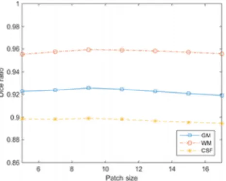
F. 5. Segmentation performance with respect to different patch sizes.
increasingly consistent with the ground truth by using the sequential random forest classifiers.
3. EXPERIMENTAL RESULTS
3.A. Parameters of random forest classifiers
The parameters of the random forest classifiers were determined via leave-one-out cross-validation on all training subjects. When optimizing a certain parameter, the other parameters were fixed. Figure 5 shows the performance with different patch sizes. We can observe that a patch size that is too small or too large will affect segmentation negatively. We therefore set the patch size as 9×9×9 in our experiments. Figure6shows the impact of the number of trees on segmentation accuracy. It can be observed that increasing the number of trees beyond 20 will not significantly improve segmentation performance. We therefore use 20 trees in each random forest in our experiments. Figure7shows the change in performance with increasing number of classifiers. In this experiment, we iteratively train the model up to 10 times to show the converge of the segmentation results. It can be seen that the Dice ratios become stable after a few iterations. In the second iteration, the Dice ratios are improved greatly due to the integration of tissue probability maps estimated in the previous iteration to guide tissue segmentation. These results also demonstrate the importance of using multiclass context features for segmentation. Note that based on Fig.7Dice ratios converge after 3 or 4 iterations; therefore, 3 or 4 iterations will be adequate in real applications.
F. 6. Segmentation performance with respect to different tree numbers.
F. 7. Changes of GM, WM, and CSF Dice ratios with respect to the number of random forest classifiers.
3.B. Comparison with other methods
We compared our method with other segmentation methods provided in the following software packages: (1) ,33 (2) Medical Image Processing, Analysis, and Visualization (),43and (3) Statistical Parametric Mapping ().44The leave-one-out cross-validation based Dice ratios for the 10 training subjects are reported in TableI. The results indicate that the proposed method outperforms other methods for all three tissue types in most cases. Specifically, for the average Dice ratio of all 10 subjects, our method performs much better than any other comparison methods. For example, compared to the best method, our method improves about 0.07 for GM, >0.03 for WM, and>0.12 for CSF.
Qualitative results for visual inspection are also shown in Figs. 8–10. From Fig. 8, we can observe that our method, compared with , , and , produces results that are significantly closer to the ground-truth segmentations. Figure 9 shows the differences of the label maps with respect to the ground-truth segmentations, indicating that the proposed method produces better segmentation with lesser false positives and false negatives.
3.C. Comparisons using the Alzheimer’s Disease Neuroimaging Initiative (ADNI) dataset
We have also applied our proposed method on 797 ADNI subjects, including 198 AD patients, 405 MCI patients, and 194 normal controls.45Demographic information of these
TI. Comparison of tissue segmentation performance in terms of Dice ratios.
Dice ratio (%) Sub. 1 Sub. 2 Sub. 3 Sub. 4 Sub. 5 Sub. 6 Sub. 7 Sub. 8 Sub. 9 Sub. 10 Mean±standard variances (pvalue)
GM
Proposed 87.54 88.81 88.78 87.94 86.33 92.62 90.72 90.31 91.38 90.45 89.49±1.83
83.39 81.85 81.32 83.09 81.03 81.07 78.75 83.07 82.13 77.57 81.33±1.80 (<0.001)a
84.31 81.74 81.66 80.56 81.92 83.89 79.70 84.47 83.43 83.85 82.55±1.58 (<0.001)a
77.39 77.58 79.71 77.75 79.53 78.81 79.60 78.01 84.63 70.21 78.32±3.36 (<0.001)a
WM
Proposed 93.80 94.18 94.26 93.25 93.45 95.90 95.27 94.07 95.62 95.36 94.52±0.90
94.15 87.96 88.60 89.98 85.17 95.29 90.13 95.00 92.76 95.87 91.49±3.46 (0.021)b
92.82 87.49 88.69 86.85 86.76 92.32 90.33 94.37 92.02 94.90 90.66±2.91 (0.001)b
82.08 79.78 81.41 81.25 80.26 83.21 87.30 83.46 84.82 84.22 82.78±2.18 (<0.001)b
CSF
Proposed 79.85 78.18 76.34 77.09 73.29 88.11 86.15 80.50 77.58 82.62 79.97±4.32
64.79 60.46 60.75 63.12 49.70 77.48 69.73 64.94 66.29 70.72 64.80±6.99 (<0.001)c
64.69 59.65 59.89 61.51 48.34 75.14 69.67 70.75 63.80 69.59 64.30±7.21 (<0.001)c
67.77 63.32 51.76 69.70 51.90 78.32 73.43 77.83 75.15 61.91 67.11±9.28 (0.001)c
Note: “a,” “b,” and “c” indicate, respectively, that the improvement in GM, WM, and CSF segmentations given by our method is statistically significant over the comparison
method according to the pairedt-test.
Regional analysis of volumes examined in normalized space (Ravens) maps were then computed from the resulting deformation field by preserving the GM/WM volume changes. Before statistical analysis, segmented images were smoothed using a Gaussian kernel with isotropic 8 mm full width at half maximum (FWHM). We then compared ravens maps of AD vs NC and MCI vs NC for their GM/WM differences.
Figures12and13show the GM/WM volume differences of AD vs NC and MCI vs NC, respectively. For the case of AD vs NC (Fig.12), in the upper row, our method andshow
significant cortical atrophy for GM, but seems to detect too much GM atrophy. In the lower row, shows larger WM volumes even in the AD patients than NC for many WM regions, which does not agree with the pathology of the brain disorder.47In contrast, our method identified reasonable WM
atrophies in many parts of brain. In Fig.13, we observe similar results for the group comparison between MCI and NC. One possible reason may be thatundersegmented GM and thus oversegmented WM (as confirmed in Fig.10), especially in AD/MCI subjects with less GM.
F. 9. The first row shows the segmentation results given by different methods. The next three rows show the differences of GM, WM, and CSF label maps with the ground-truth segmentation. Black and white denote false negatives and false positives, respectively.
To further evaluate the sensitivity of the methods, we performed another experiment on a typical AD-related brain region, namely, the hippocampus. Specifically, we first delin-eated the ROI for the left and right hippocampi and then extracted the mean ravens value in the ROI for each subject from the proposed method and the comparison method. Through a two-samplet-test, we compared the mean ravens value in the hippocampi between AD and NC. The values
given by the proposed method show significant differences between groups (t=−4.64 and p=4.83×10⁻⁶). Here the negative t value indicates that AD patients have relatively lower ravens value than NC, reflecting smaller hippocampal volume. However, when using the ravens values from the
method, no significant difference is found (t=−0.83 and
p=0.403). These results suggest that our proposed method is more sensitive in identifying hippocampal atrophy.
TII. Demographic information of participants involved in ADNI study.
AD MCI Normal control
No. of subjects 198 405 194
No. of males 103 266 119
Age (yr, mean±SD) 75.6±7.7 74.8±7.5 75.9±5.0
F. 10. Comparison of segmentation results on the ADNI dataset with different methods. The first column shows the original T1-weighted MR image slices and
the second and third columns show the segmentation results given by the proposed method and, respectively. The second to fourth rows show the close-up
views of the areas marked in the first row.
F. 11. Comparison of renderings of GM/CSF (first and third) and GM/WM (second and fourth) surfaces generated from the segmentation results on one
ADNI image given by the proposed method (first two columns) and themethod (last two columns) in the first row. The corresponding close-up views are
also shown in the second row.
F. 12. Group differences between AD and NC. Upper row: GM volume differences given by the proposed method (left) and themethod (right). Lower
row: WM volume differences given by the proposed method (left) andmethod (right). Red/blue color denotes expansion/atrophy, respectively (p<0.05
F. 13. Group differences between MCI and NC. Upper row: GM volume differences given by the proposed method (left) andmethod (right). Lower row:
WM volume differences given by the proposed method (left) andmethod (right). Red/blue color denotes expansion/atrophy, respectively (p<0.05 FDR
corrected, cluster size>50). (See color online version.)
3.D. Computational time
The experiments were carried out on a computing cluster with 2.93 GHz Intel processors, 12 M L3 cache, and 48 GB memory. All trees in the RF are trained in parallel with an average training time of about 1.5 h per tree. It took about 5 min to segment a typical 3T brain MR image.
4. DISCUSSIONS AND CONCLUSION
In this paper, we presented a method for robust and accurate segmentation of 3T T1-weighted MR images by learning segmentation information from their corresponding 7T MR images. The proposed algorithm combines information from T1-weighted MR images and tentatively estimated tissue probability maps. First, we trained the random forest classifier with 3T brain MR images and their ground-truth tissue segmentations obtained from their corresponding 7T MR images. Then, in the next iterations, the proposed automatic segmentation algorithm integrates both the T1-weighted MR image and the probability maps of GM, WM, and CSF estimated in the last iteration to train the next random forest classifier that progressively refines the tissue probability maps. Results using various datasets confirm that the proposed method can consistently improve segmentation performance. Recently, deep learning has demonstrated state-of-the-art performances in various applications, such as classification,48
voice recognition,49 and segmentation.16 In contrast to the
handcrafted features (Haar-like features) used in our method, deep learning algorithms automatically learn relevant features from the images. The convolutional neural network (CNN), for example, has been employed for segmentation.50Deep learning algorithms can also benefit from accurate segmentation infor-mation provided by 7T MRI for improving feature learning.51 Although our method produces better segmentation results, it has some limitations. (1) The number of training subjects (with both 3 and 7T MR images) is small in our experiments. With more training subjects, the segmentation accuracy can be improved. (2) Age-specific information is not considered in our work. For example, the 10 training subjects are 30±8 yr of age, which are different from the ADNI subjects who are mostly over 60 yr old. The results can be improved if the age ranges match. (3) The training subjects consist of healthy persons and epilepsy patients, while the most ADNI
subjects are the patients with Alzheimer’s disease (AD) or Mild Cognitive Impairment (MCI). (4) We used Haar-like features. Other types of features might be more effective.
ACKNOWLEDGMENTS
This work was supported in part by the 2013 Natu-ral Science Program of Heilongjiang Province Educational Committee (No. 12531011), the Abroad Research Project of Heilongjiang Province University Strategic Reserve Talent, the Research Fund for the Doctoral Program of Higher Education of China (RFDP) (No. 20133219110029), and the China Scholarship Council (No. 201506840071). This work was also supported in part by National Institutes of Health Grant Nos. MH100217, MH070890, EB006733, EB008374, EB009634, AG041721, AG042599, and MH088520. ADNI Data used in preparation of this article were obtained from the Alzheimer’s Disease Neuroimaging Initiative (ADNI) database (adni.loni.ucla.edu). As such, the investigators within the ADNI contributed to the design and implementation of ADNI and/or provided data but did not participate in analysis or writing of this report. A complete listing of ADNI inves-tigators can be found at:http://adni.loni.ucla.edu/wp-content/ uploads/how_to_apply/ADNI_Acknowledgement_List.pdf.
CONFLICT OF INTEREST DISCLOSURE The authors have no COI to report.
a)M. Deng and R. Yu contributed equally to this study and should be
considered as co-first authors.
b)Author to whom correspondence should be addressed. Electronic mail:
1B. Caldairou, N. Passat, P. A. Habas, C. Studholme, and F. Rousseau, “A
non-local fuzzy segmentation method: Application to brain MRI,”Pattern
Recognition44, 1916–1927 (2011).
2L. G. Apostolova, G. G. Akopyan, N. Partiali, C. A. Steiner, R. A. Dutton, K.
M. Hayashi, I. D. Dinov, A. W. Toga, J. L. Cummings, and P. M. Thompson,
“Structural correlates of apathy in Alzheimer’s disease,”Dement. Geriatr.
Cogn. Disord.24, 91–97 (2007).
3L. Clare, R. T. Woods, E. D. Moniz Cook, M. Orrell, and A. Spector,
“Cognitive rehabilitation and cognitive training for early-stage Alzheimer’s
disease and vascular dementia,”Cochrane Database Syst. Rev.4, 7 (2003).
4J. G. Csernansky, L. Wang, S. Joshi, J. P. Miller, M. Gado, D. Kido, D.
McKeel, J. C. Morris, and M. I. Miller, “Early DAT is distinguished from aging by high-dimensional mapping of the hippocampus dementia of the
5J. Morraet al., “Automated 3D mapping of hippocampal atrophy and its
clinical correlates in 400 subjects with Alzheimer’s disease, mild
cogni-tive impairment, and elderly controls,”Hum. Brain Mapp.30, 2766–2788
(2009).
6J. J. Lin, N. Salamon, R. A. Dutton, A. D. Lee, J. A. Geaga, K. M. Hayashi,
A. W. Toga, and J. Engel, Jr., “Three-dimensional preoperative maps of hippocampal atrophy predict surgical outcomes in temporal lobe epilepsy,” Neurology65, 1094–1097 (2005).
7R. Nicolson, T. DeVito, C. N. Vidal, Y. Sui, K. M. Hayashi, D. J. Drost, P. C.
Williamson, N. Rajakumar, A. W. Toga, and P. M. Thompson, “Detection
and mapping of hippocampal abnormalities in autism,”Psychiatry Res.148,
11–21 (2006).
8P. M. Thompsonet al., “Mapping hippocampal and ventricular change in
Alzheimer disease,”NeuroImage22, 1754–1766 (2004).
9C. E. Beardenet al., “Three-dimensional mapping of hippocampal anatomy
in unmedicated and lithium-treated patients with bipolar disorder,”
Neu-ropsychopharmacology33, 1229–1238 (2007).
10X. Han and B. Fischl, “Atlas renormalization for improved brain MR image
segmentation across scanner platforms,”IEEE Trans. Med. Imaging26,
479–486 (2007).
11Y. Chen, B. Zhao, J. Zhang, and Y. Zheng, “Automatic segmentation for
brain MR images via a convex optimized segmentation and bias field
correc-tion coupled model,”Magn. Reson. Imaging32, 941–955 (2014).
12J. Morra, Z. Tu, L. G. Apostolova, A. Green, A. Toga, and P.
Thomp-son, “Comparison of AdaBoost and support vector machines for detecting
Alzheimer’s disease through automated hippocampal segmentation,”IEEE
Trans. Med. Imaging29, 30–43 (2007).
13S. Powell, V. Magnotta, H. Johnson, V. K. Jammalamadaka, R. Pierson,
and N. C. Andreasen, “Registration and machine learning-based automated
segmentation of subcortical and cerebellar brain structures,”NeuroImage
39, 238–247 (2008).
14A. Pitiot, H. Delingette, P. M. Thompson, and N. Ayache, “Expert
knowledge-guided segmentation system for brain MRI,”NeuroImage23,
S85–S96 (2004).
15P. Golland, W. Grimson, M. E. Shenton, and R. Kikinis, “Detection and
analysis of statistical differences in anatomical shape,”Med. Image Anal.
9, 69–86 (2005).
16W. Zhang, R. Li, H. Deng, L. Wang, W. Lin, S. Ji, and D. Shen, “Deep
convolutional neural networks for multi-modality isointense infant brain
image segmentation,”NeuroImage108, 214–224 (2015).
17E. Y. Kim, “Machine-learning based automated segmentation tool
devel-opment for large-scale multicenter MRI data analysis,” (The University of Iowa, 2013).
18A. Joy, S. Roy, J. L. Prince, and A. Carass, “MR brain segmentation using
decision trees,” MR Brains13(2013).
19J. Mitra, P. Bourgeat, J. Fripp, S. Ghose, S. Rose, O. Salvado, B. C.
Alan Connelly, S. Palmer, G. Sharma, S. Christensen, and L. Carey, “Le-sion segmentation from multimodal MRI using random forest following
ischemic stroke,”NeuroImage98, 324–335 (2014).
20S. Pereira, J. Festa, J. A. Mariz, N. Sousa, and C. A. Silva, “Automatic
brain tissue segmentation of multi-sequence MR images using random
decision forests,” inProceedings of the MICCAI Grand Challenge on MR
Brain Image Segmentation(MRBrainS’13, 2013), Vol. 6.
21L. Wang, F. Shi, Y. Gao, G. Li, J. H. Gilmore, W. Lin, and D. Shen,
“Integra-tion of sparse multi-modality representa“Integra-tion and anatomical constraint for
isointense infant brain MR image segmentation,”NeuroImage89, 152–164
(2014).
22J. Rauschenberg, “7T & higher-human safety the path to the clinic adoption,”
Proc. Intl. Soc. Magn. Reson. Med.19(2011).
23M. Bernstein, J. Huston, and H. Ward, “Imaging artifacts at 3.0 T,”J. Magn.
Reson. Imaging24, 735–746 (2006).
24A. Hahn, G. S. Kranz, E. M. Seidel, R. Sladky, C. Kraus, M. Küblböck,
D. M. Pfabigan, A. Hummer, A. Grahl, S. Ganger, C. Windischberger, C. Lamm, and R. Lanzenberger, “Comparing neural response to painful
electrical stimulation with functional MRI at 3 and 7 T,”NeuroImage82,
336–343 (2013).
25R. Sladky, P. Baldinger, G. S. Kranz, J. Tröstl, A. Höflich, R. Lanzenberger,
E. Moser, and C. Windischberger, “High-resolution functional MRI of the
human amygdala at 7 T,”Eur. J. Radiol.82, 728–733 (2013).
26J. Braun, J. Guo, R. Lützkendorfc, J. Stadlerc, S. Papazogloub, S. Hirschb,
I. Sackb, and J. Bernarding, “High-resolution mechanical imaging of the human brain by three-dimensional multifrequency magnetic resonance
elas-tography at 7T,”NeuroImage90, 308–314 (2014).
27P. Martín-Vaquero, D. COSTA, R. L. Echandi, C. L. Tosti, M. V. Knopp, and
S. Sammet, “Magnetic resonance imaging of the canine brain at 3 and 7 T,” Vet. Radiol. Ultrasound52, 25–32 (2011).
28D. Zikic, B. Glocker, and A. Criminisi, “Encoding atlases by randomized
classification forests for efficient multi-atlas label propagation,”Med. Image
Anal.18, 1262–1273 (2014).
29D. Zikic, B. Glocker, E. Konukoglu, A. Criminisi, C. Demiralp, J. Shotton,
O. M. Thomas, T. Das, R. Jena, and S. J. Price, “Decision forests for
tissue-specific segmentation of high-grade gliomas in multi-channel MR,”Med.
Image Comput. Comput. Assisted Intervention2012, 369–376.
30F. Shi, L. Wang, Y. Dai, J. H. Gilmore, W. Lin, and D. Shen, “LABEL:
Pe-diatric brain extraction using learning-based meta-algorithm,”NeuroImage
62, 1975–1986 (2012).
31J. G. Sled, A. P. Zijdenbos, and A. C. Evans, “A nonparametric method for
automatic correction of intensity nonuniformity in MRI data,”IEEE Trans.
Med. Imaging17, 87–97 (1998).
32T. S. Yoo, M. J. Ackerman, W. E. Lorensen, W. Schroeder, V. Chalana,
S. Aylward, D. Metaxas, and R. Whitaker, “Engineering and algorithm design for an image processing API: A technical report on ITK—The insight
toolkit,”Stud. Health Technol. Inform.85, 586–592 (2002).
33Y. Zhang, M. Brady, and S. Smith, “Segmentation of brain MR
im-ages through a hidden Markov random field model and the expectation–
maximization algorithm,”IEEE Trans. Med. Imaging20, 45–57 (2001).
34P. A. Yushkevich, J. Piven, H. C. Hazlett, R. G. Smith, S. Ho, J. C. Gee,
and G. Gerig, “Userguided 3D active contour segmentation of anatomical
structures: Significantly improved efficiency and reliability,”NeuroImage
31, 1116–1128 (2006).
35L. Breiman, “Bagging predictors,”Mach. Learn.24, 123–140 (1996).
36T. Ho, “The random subspace method for constructing decision forests,”
IEEE Trans. Pattern Anal. Mach. Intell.20, 832–844 (1998).
37Y. Amit and D. German, “Shape quantization and recognition with
random-ized trees,”Neural Comput.9, 1545–1588 (1997).
38L. Breiman, “Random forests,”Mach. Learn.45, 5–32 (2001).
39J. Maiora, B. Ayerdi, and M. Graña, “Random forest active learning for AAA
thrombus segmentation in computed tomography angiography images,” Neurocomputing126, 71–77 (2014).
40A. Pinto, S. Pereira, H. Dinis, and C. A. Silva, “Random decision forests
for automatic brain tumor segmentation on multi-modal MRI images,” in 2015 IEEE 4th Portuguese BioEngineering Meeting Porto (IEEE, Portuguese, 2015), Vol. 3.
41H. Cheng, Z. Liu, and L. Yang, “Sparsity induced similarity measure
for label propagation,” in2009 IEEE 12th International Conference on
Computer Vision(IEEE, Kyoto, Japan, 2009), Vol. 8.
42J. Wright, A. Y. Yang, A. Ganesh, S. S. Sastry, and Y. Ma, “Robust face
recognition via sparse representation,”IEEE Trans. Pattern Anal. Mach.
Intell.31, 210–227 (2009).
43N. R. Pal and S. K. Pal, “A review on image segmentation techniques,”
Pattern Recognition26, 1277–1294 (1993).
44J. Ashburner, G. Barnes, C. Chen, J. Daunizeau, G. Flandin, K. Friston,
D. Gitelman, S. Kiebel, J. Kilner, and V. Litvak,8Manual(Functional
Imaging Laboratory, Institute of Neurology,41(2008)).
45C. R. Jack, M. A. Bernstein, N. C. Fox, P. Thompson, G. Alexander, D.
Harvey, B. Borowski, P. J. Britson, J. L. Whitwell, and C. Ward, “The
Alzheimer’s disease neuroimaging initiative (ADNI): MRI methods,”J.
Magn. Reson. Imaging27, 685–691 (2008).
46D. Shen and C. Davatzikos, “HAMMER: Hierarchical attribute
match-ing mechanism for elastic registration,”IEEE Trans. Med. Imaging21,
1421–1439 (2002).
47R. Peters, “Ageing and the brain,”Postgrad. Med. J.82, 84–88 (2006).
48D. C. Ciresan, U. Meier, J. Masci, L. Maria Gambardella, and J.
Schmidhu-ber, “Flexible, high performance convolutional neural networks for image
classification,”IJCAI Proceedings-International Joint Conference on
Arti-ficial Intelligence22, 1237 (2011).
49L. Deng, O. Abdel-Hamid, and D. Yu, “A deep convolutional neural network
using heterogeneous pooling for trading acoustic invariance with phonetic
confusion,”IEEE International Conference on Acoustics, Speech and Signal
Processing6669–6673 (2013).
50J. Long, E. Shelhamer, and T. Darrell, “Fully convolutional networks for
semantic segmentation,”Proceedings of the IEEE Conference on Computer
Vision and Pattern Recognition3431–3440 (2015).
51D. L. Richmond, D. Kainmueller, M. Yang, E. W. Myers, and C. Rother,
“Mapping stacked decision forests to deep and sparse convolutional neural