GEOSTATISTICAL ESTIMATION OF WATER QUALITY USING RIVER
AND FLOW COVARIANCE MODELS
Prahlad Jat
A dissertation submitted to the faculty of the University of North Carolina at Chapel Hill in partial fulfillment of the requirements for the degree of Doctor of Philosophy in the Department
of Environmental Sciences and Engineering.
Chapel Hill 2016
Approved by: Marc L. Serre
Gregory W. Characklis
Jacqueline MacDonald Gibson William Vizuete
ii © 2016 Prahlad Jat
iii
ABSTRACT
Prahlad Jat: Geostatistical Estimation of Water Quality using River and Flow Covariance Models (Under the direction of Marc L. Serre)
Assessing water quality along rivers is vital for watershed management and to protect the public health. Monitoring water quality at every river mile is logistically impractical and prohibitively expensive. Geostatistical estimation offers a cost effective alternative that can be rapidly implemented to statistically model spatially dependent water quality parameters using the available monitoring data. Geostatistical modeling requires a covariance model to describe the variability and autocorrelation of the water quality along rivers. Three main classes of covariance models, namely the Euclidean, river, and flow-weighted covariance models, are commonly used in geostatistical water quality estimation.
iv
v
vi
ACKNOWLEDGEMENTS
First and foremost I would like to express my deepest gratitude to my advisor, Marc Serre, for his guidance, inspiration and support during my tenure as a PhD student. I feel extremely privileged to work with Marc and I have learned a great deal from him, above and beyond his contributions to my research. He has always been willing to delve into the details of the work and talk through issues, sometimes long past a reasonable meeting length. I am very thankful to all of my doctoral committee members: Profs Gregory W. Characklis, Jacqueline MacDonald Gibson, William Vizuete, and Lawrence E. Band. Each of them offered great insight and suggestions that have enhanced this body of work.
Last, but not least, I would like to thank my loving family and friends for their
vii
TABLE OF CONTENTS
LIST OF TABLES ... xii
LIST OF FIGURES ... xiii
CHAPTER 1 : INTRODUCTION ... 1
1. Literature review of geostatistical estimation of river water quality ... 1
2. Classes of covariance models used to study water quality ... 4
2.1. Autocorrelation in water quality ... 4
2.2. Euclidean covariance model ... 7
2.3. River covariance model ... 8
2.4. Flow-weighted covariance model ... 9
2.5. Mixture of Euclidean and flow covariance models ... 11
3. Some Knowledge gaps in previous water quality studies ... 13
4. Research objectives ... 15
4.1. Research objective 1: Bayesian Maximum Entropy Space/time Estimation of Surface Water Chloride in Maryland Using River Distances ... 15
4.2. Research objective 2: Introducing a novel geostatistical approach combining Euclidean and flow-weighted covariance models to estimate fecal coliform along the Deep and Haw Rivers in North Carolina ... 16
4.3. Research objective 3: Bayesian Maximum Entropy Space/time Estimation of Surface Water Chloride in Maryland Using River Distances ... 18
CHAPTER 2 (PAPER 1): BAYESIAN MAXIMUM ENTROPY SPACE/TIME ESTIMATION OF SURFACE WATER CHLORIDE IN MARYLAND USING RIVER DISTANCES1 ... 20
viii
2. Materials and Methods ... 22
2.1. Chloride and Hydrography Data ... 22
2.2. Left-Censored Data ... 23
2.3. Space/time BME Geostatistical Framework for Mapping Analysis ... 24
2.4. Comparison of BME using River versus Euclidean Distance ... 29
2.5. Sensitivity Analysis with respect to the Proportion of Left Censored Data ... 30
2.6. Assessment of Impaired River Miles ... 31
3. Results and Discussion ... 31
3.1. Covariance Models of Offset-Removed Chloride log-Concentrations ... 31
3.2. Cross-Validation Results Contrasting the Euclidean versus River Covariance models ... 32
3.3. Cross-Validation Results Contrasting Euclidean versus River Offsets ... 33
3.4. Sensitivity Analysis Results with respect to Censoring Limit ... 34
3.5. Cross Validation Results Contrasting the River and LUR Offsets ... 35
3.6. Difference in the Maps Produced Using Euclidean versus River BME ... 36
3.7. Space/time Patterns in Chloride Contamination ... 39
3.8. Probabilistic Assessment of Impaired River Miles ... 41
4. Conclusions ... 42
Acknowledgements ... 44
REFERENCES ... 45
CHAPTER 3 (PAPER 2): A NOVEL GEOSTATISTICAL APPROACH COMBINING EUCLIDEAN AND GRADUAL-FLOW COVARIANCE MODELS TO ESTIMATE FECAL COLIFORM ALONG THE HAW AND DEEP RIVERS IN NORTH CAROLINA2 ... 49
ix
2. Materials and Methods ... 51
2.1. Fecal coliform and hydrography Data ... 51
2.2. Space/time Bayesian Maximum Entropy geostatistical framework ... 53
2.3. Euclidean covariance model ... 54
2.4. River covariance model ... 55
2.5. Flow-weighted covariance model using pipe flow ... 56
2.6. Flow-weighted covariance model using gradual flow ... 58
2.7. Hybrid Euclidean-flow covariance model ... 60
2.8. Calculating experimental covariance values ... 61
2.9. Model performance evaluation and assessment of river miles with high fecal coliform…. ... 62
3. Results and Discussion ... 63
3.1. The hybrid Euclidean/Gradual-flow estimates are more accurate than those obtained using a purely Euclidean or purely flow-weighted covariance model ... 63
3.2. When using a coarse river network, the Euclidean/gradual-flow estimates are more accurate than the Euclidean/pipe-flow estimates ... 64
3.3. Fecal coliform concentrations vary over long spatial distances and short time scales ... 65
3.4. Euclidean/Gradual-flow estimates reveal that fecal contamination is more watershed specific and covers more river miles than traditionally thought ... 67
3.5. Euclidean/Gradual-flow estimates capture hydrological transport ... 67
3.6. The Euclidean/Gradual-flow model substantially increases sensitivity in the detection of fecal impairment ... 68
3.7. Concluding remarks and future works ... 70
x
REFERENCES ... 71
CHAPTER 4 (PAPER 3): SPACE/TIME ESTIMATION OF DISSOLVE ORGANIC CARBON ALONG RIVERS IN MARYLAND USING A COMBINATION OF EUCLIDEAN AND FLOW-WEIGHTED COVARIANCE MODELS3 ... 74
1. Introduction ... 74
2. Materials and Methods ... 77
2.1. DOC and hydrography data ... 77
2.2. Space/time Bayesian Maximum Entropy framework ... 78
2.3. Spatial covariance model ... 80
2.4. Calculating experimental covariance values and selecting covariance parameters ... 81
2.5. Accuracy of model estimates and probabilistic assessment of DOC impaired river miles ... 82
3. Results and Discussion ... 83
3.1. The Euclidean model is more accurate than the river and the flow models, indicating that terrestrial sources is the primary driver of DOC variability along rivers ... 83
3.2. The hybrid Euclidean/Gradual-flow model is the most accurate model, indicating that flow plays a role in the distribution of DOC along rivers ... 84
3.3. The domain wide variability of DOC is watershed specific ... 86
3.4. The fine scale variability of DOC is influenced by hydrological transport along individual river reaches and by dilution at confluence points ... 88
3.5. There is a small fraction of impaired river miles but a large fraction of unassessed river miles ... 89
REFERENCES ... 91
CHAPTER 5: CONCLUSIONS ... 94
xi
NHD Flowlines in Subbasins ... 97
Impervious Surface Data... 98
Land Use Regression (LUR) Model ... 99
Offset models ... 100
Weighted Least Square Covariance Fitting Procedure ... 103
Sensitivity Analysis with Respect to the Proportion of Left Censored Data ... 105
Maps and Movies ... 106
BME Estimate of chloride concentration ... 106
BME estimate of the probability that chloride exceeds 230 (mg/l) ... 107
REFERENCES ... 109
APPENDIX B: SUPPLEMENTAL INFORMATION FOR ‘A NOVEL GEOSTATISTICAL APPROACH COMBINING EUCLIDEAN AND GRADUAL-FLOW COVARIANCE MODELS TO ESTIMATE FECAL COLIFORM ALONG THE HAW AND DEEP RIVERS IN NORTH CAROLINA’ PAPER ... 110
Details on the fecal coliform and hydrography data ... 110
Details on the flow-weighted covariance models using pipe flow ... 112
Derivation of the flow-weighted covariance model using gradual flow... 113
Leave-One-Out Cross-Validation (LOOCV) statistics ... 114
Pipe flow is a poor approximation of gradual flow along a coarse river network representation of the Haw and Deep rivers ... 115
Modeling the spatial covariance using Euclidean distance, river distance, and flow ratio ... 116
Daily estimates of fecal coliform across the study area ... 120
Number of impaired river miles ... 122
xii
LIST OF TABLES
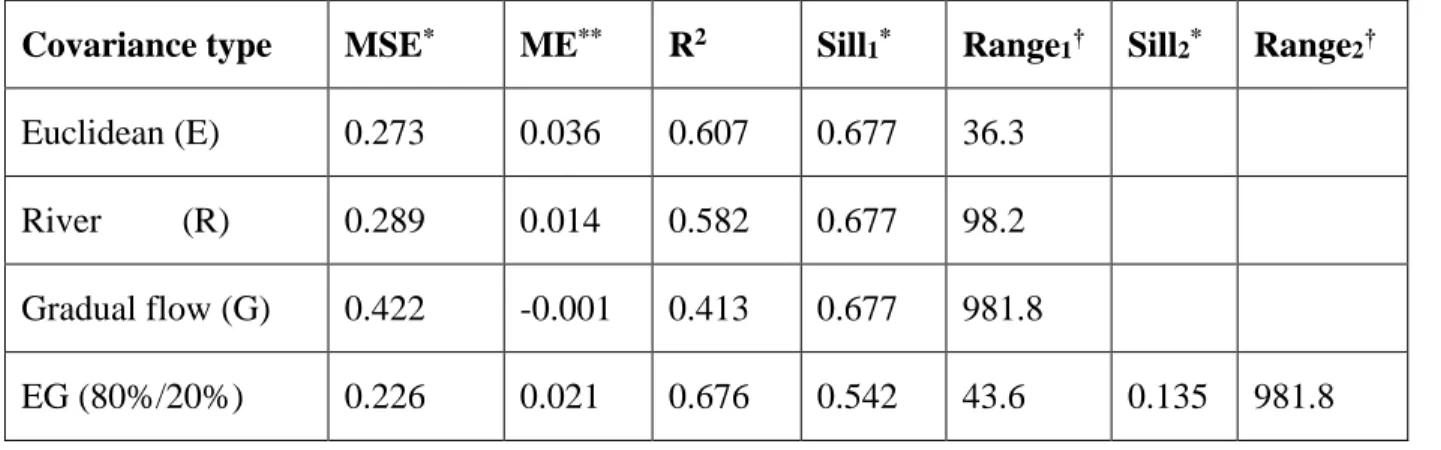
Table 2.1: Leave-one-out cross-validation statistics obtained using the BME method with different offset and covariance models for the estimation of chloride log-concentration... 33 Table 4. 1: Leave-one-out cross-validation statistics and corresponding covariance
parameter values obtained using the (E) Euclidean, (R) River, (G) Gradual-flow, (EG) Euclidean/Gradual-flow covariance models. For the E, R, and G models, Sill1 and Range1 are the covariance sill (σ2) and range (aE, aR, aG for
the E, R, G model respectively) obtained through least square fitting. For the EG model Sill1= αEσ2 and Range1=aE are the covariance sill and range of the
Euclidean model, and Sill2= αGσ2 and Range2=aG are the covariance sill and
range of the flow covariance model. For the EG model, αE and αG are obtained by selecting the αE that minimizes the cross-validation MSE, resulting in
αE=80% and αG=20%. In all models, the temporal range is at =7 years ... 84
Table A.S1: Subbasin name, number of NHD flowlines, stream length, and area of the subbasin in our study domain (Source: ArcView analysis- 1:24,000 scale NHD hydrography dataset1.) ... 97 Table A.S2: Sensitivity analysis of the estimation accuracy of the river BME and
kriging methods with respect to the proportion of left censored data ... 106 Table B.S1: Descriptive statistics of fecal coliform concentrations observed along the
Haw and Deep rivers in North Carolina from 2006-2010 ... 111 Table B.S2: Number of impaired river miles estimated using the Euclidean covariance
xiii
LIST OF FIGURES
Figure 1.1: Schematic representation of how the autocorrelation in terrestrial contamination sources and the longitudinal transport distance along rivers can lead to various water quality covariance models: (a) contamination source autocorrelated across long Euclidean distances coupled with transport over short distances can lead to an Euclidean covariance model, (b) source
autocorrelated along long river distances and transport over short distances can lead to a river covariance model, (c) point sources autocorrelated over short distances and transport along long river distances can lead to a flow covariance model and (d) contamination source autocorrelated across long Euclidean distances coupled with transport along long distances can lead to nested Euclidean-flow covariance model. For each covariance model the correlation
between 4 sites (labeled 2 to 5) and site 1 is shown using color darkness. ... 6 Figure 2.2: Cross validation MSE for river BME and its kriging linear limiting cases
shown with respect to the proportion of censored data. BME (method a) rigorously models the uncertainty in the censored data using the TGPDF, while kriging treats them as data with no uncertainty by simply replacing them with half of the CL (method b) or by the CL (method c). ... 35 Figure 2.3: Maps of the BME mean estimate of chloride concentrations in 2014.
The maps on the left panels are estimated using Euclidean BME, the maps on the right are estimated using river BME. Panel (a), (c) and (e) show the Euclidean BME estimate of chloride in area B, area C, and the study domain, respectively. The corresponding river BME maps are in the Panels (b), (d) and (g), respectively. The flow lines in panels (a), (b), (c), and (d) are highlighted (increased width) for better visual appearances of segments compared for estimation accuracy. The width of the flow lines in panels (e) and (f) correspond to their cumulative river miles. ... 38 Figure 2.4: Time series of average fraction of river miles in Gunpowder-Patapsco, Patuxent,
and Severn subbasins in Maryland that are highly likely in non-attainment (the probability of exceedance of the EPA guideline (230 mg/l) is greater than 90 %), non-assessed (probability between 10% and 90%), and highly likely in attainment (probability less than 10%) from 2005 to 2014. See Supplementary Information for maps showing for each year from 2005 to 2014 the spatial distribution of the
probability that chloride exceeds 230 (mg/l). ... 42 Figure 3.1: Panel (a) shows a map of the study area depicting the fecal coliform observation
xiv
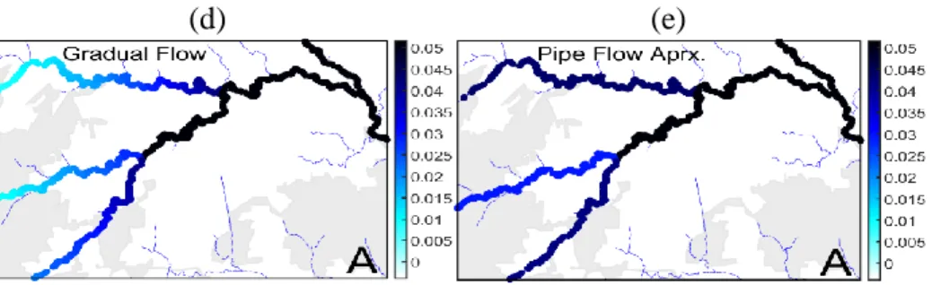
Likewise, the gradual flow along the coarse river network shown in panel (d) for area A is poorly approximated by its corresponding pipe flow shown in panel (e). In particular the pipe flow along the upstream branches of area A are not able to reproduce well the gradual flow in these reaches. ... 53 Figure 3.2: Maps of fecal coliform estimates (CFU/100ml) obtained on 12-Jun-2006 across
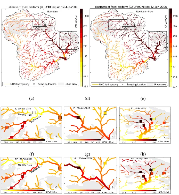
the study area are shown in panels (a) and (b), those obtained on 25-Feb-2010 over area A are shown in panels (c) and (f), those obtained on 05-Jan-2010 over area B are shown in panels (d) and (g), and those obtained on 14-Sep-2007 over area C are shown in panels (e) and (h). Estimates obtained using the Euclidean covariance model are shown in panels (a), (c), (d) and (e) while those obtained using the
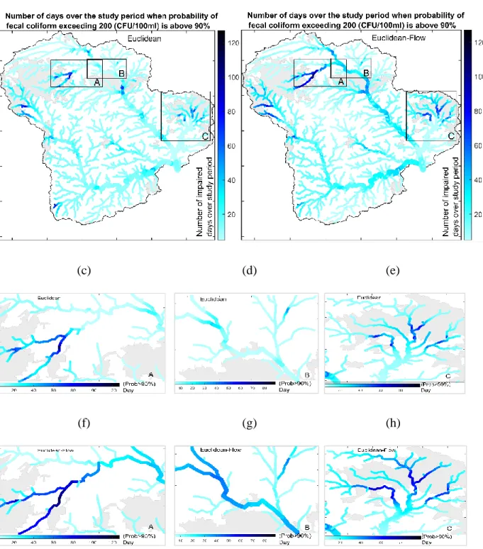
Euclidean/Gradual-flow covariance model are shown in panels (b), (f), (g), and (h). ... 66 Figure 3.3 : These maps show, for each river mile, the number of sampling days (out of a
total of 573 sampling days in 2006-2010) assessed as having high fecal coliform (i.e. with Prob[FC>200CFU/100ml]>90%). The study area is shown in panels (a) and (b), area A is shown in panels (c) and (f), area B is shown in panels (d) and (g), and area C is shown in panels (e) and (h). Estimates obtained using the Euclidean covariance model are shown in panels (a), (c), (d) and (e) while those obtained using the Euclidean/Gradual-flow covariance model are shown in panels (b), (f), (g), and (h). ... 69 Figure 4.1: Map of the study area depicting Maryland Biological Stream Survey
(MBSS) monitoring sites in the Gunpowder-Patapsco, Patuxent, and Severn sub-basins in Maryland. ... 78 Figure 4.2: (a) Plot of the MSE as a function of αE, the proportion of the Euclidean
component in the hybrid Euclidean/Gradual-low covariance model. Experimental covariance values (markers) and Euclidean/Gradual-flow covariance model (lines) shown as a function of (b) Euclidean lag for a fixed river lag and fixed flow ratios, and (c) as a function of flow ratio for fixed Euclidean and river lags. ... 85 Figure 4.3: Panels (a) and (b) show the maps depicting the spatial distribution of DOC
(mg/l) across the study domain in 2013 obtained using Euclidean and
Euclidean/Gradual-flow models, respectively. Panels (c) and (d) are maps of estimates obtained using Euclidean and Euclidean/Flow models, respectively, showing the spatial distribution of DOC in 2008 near the confluence of the North and South branches of the Patapsco River. The map depicting the probability that DOC exceeds 3mg/l in 2010 is shown in panel (e), and the probabilistic assessment of DOC impairment over the study domain from 2005 to 2014 is shown in panel (f). Both panel (e) and (f) were obtained using
Euclidean/Gradual-flow covariance model. ... 88 Figure A.S1: Figure A.S1: Multi-Resolution Land Characteristics based percent
xv
Figure A.S2: Regression plot of log –chloride versus subwatershed imperviousness percentage ... 100 Figure A.S3: Spatial component of the global offset calculated using kernel smoothing
of time averaged chloride concentration measurements using an exponential kernel
function based on (a) Euclidean distances and (b) river distances. ... 102 Figure A.S4: Temporal component of the offset, obtained using an exponential kernel
smoothing of spatially averaged chloride log-concentrations ... 102 Figure A.S5: Offset of chloride concentration calculated as the LUR estimate obtained
based on a linear regression between chloride log-concentrations and HEC12
subwatershed imperviousness percentages. ... 103 Figure B.S1: Experimental covariance values obtained using gradual flow and shown
as a function of (a) Euclidean lag for fixed river lags and flow ratios, and (b) as a function of flow ratio for fixed Euclidean and river lags. The experimental covariance values obtained with pipe flow are shown in (c) with respect to flow ratio. ... 119 Figure B.S2: Maps of fecal coliform estimates (CFU/100ml) obtained using the
Euclidean covariance on 08-May-2006 (panel a) and 09-May-2006 (panel c). Estimates obtained using the Euclidean/Gradual-flow covariance model are shown in panels (b) and (d). ... 121 Figure B.S3: Maps of fecal coliform estimates (CFU/100ml) obtained on 28-Dec-2006
using the Euclidean covariance (panel a) and the Euclidean/Gradual-flow
covariance model panel (b). ... 122 Figure B.S4: Maps of the fecal coliform estimates averaged across the 2006-2010
study period are shown in panel (a) using estimates obtained with Euclidean covariance and in panel (b) using estimates obtained with Euclidean/Gradual-flow
1
CHAPTER 1 : INTRODUCTION
1.
Literature review of geostatistical estimation of river water quality
Surface water quality is an essential component of the natural environment.
Characterizing the surface water quality is often a daunting task, but it is an important one in verifying whether the observed water quality is suitable for its intended purpose and to meet the requirements of Section 305(b) of the Clean Water Act (1972). Monitoring water quality helps to determine trends and patterns in the water affected by the release of contaminants or due to other natural and anthropogenic activities. However, high monitoring costs limit
the implementation of exhaustive water quality monitoring programs and therefore probability-based water quality surveys are typically needed to do the water quality assessment needed to meet the Clean Water Act requirements (Peterson et al., 2006). EPA’s National Water Quality Inventory Report 2004 (EPA, 2009) stated that about 44% of streams, 64% of lakes, and 30% of estuaries assessed were not clean enough to meet the intended purposes in spite of the progress in cleaning up the nation’s water.
2
kriging techniques or other interpolation and regression based methods with an Euclidean distance (Rasmussen et al., 2005; Tortorelli and Pickup, 2006; Cressie et al., 2005; Peterson and Urquhart, 2006).
Water quality is often dynamic and changes rapidly in space and time. Such space-time variability of water quality cannot be captured using purely spatial models. In the case of many water quality parameters, temporal variability plays a key role in understanding the overall impact on a basin-wide system. Hence, recent developments in geostatistics have moved beyond the purely spatial approach to include temporal variability as well (Stein 1986, Christakos 1992, Bogaert 1996, Kyriakidis and Journel 1999, Fuentes 2004, Kolovos et al. 2004). Space/time geostatistical models extend the concept of autocorrelation between nearby sites from the spatial dimension into the spatial and temporal dimensions, and they produce more accurate estimates at unmonitored space/time locations.
3
spatial approach. This substantial improvement could most likely be due to the irregularity of the spatial and temporal sampling of PCE data.
Traditionally geostatistical water quality studies have used Euclidean distances to describe spatial autocorrelation (Rasmussen et al., 2005; Tortorelli and Pickup, 2006; Cressie et al., 2005; Peterson and Urquhart, 2006). Many studies have raised questions about the use of an Euclidean distance metric in the estimation of water quality along stream networks as it may fail to account for stream network topology (Money et al., 2009a). There have been several recent studies which proposed to use the river distance, i.e. the shortest distance along the river between sites, as an alternative to the Euclidean distance when studying the spatial autocorrelation
amongst stream monitoring sites. This distance is called the “hydrologic distance” (Peterson et al., 2007), “stream distance” (Ver Hoef et al., 2006), “river distance” (Cressie et al., 2006; Money, 2009a) in the recent literature. Money et al., (2009b) reported that the use of the river distance in modeling the autocorrelation in fecal contamination along the Raritan River in New Jersey resulted in lower estimation errors compared to using the Euclidean distance. However, simply replacing the Euclidean distance with the hydrologic distance may violate geostatistical modelling assumptions and may yield an invalid (i.e., non-positive-definite) model of spatial statistical dependence. Ver Hoef et al., (2006) showed that the hydrologic distance with the spherical covariance model resulted in negative eigenvalues of the covariance matrix and hence the variances can be negative too. First Ver Hoef et al., (2006) and later Money et al., (2009a) showed that using the exponential covariance model with the river distance is a valid and permissible model.
In some mapping studies the river distance alone may not fully incorporate the
4
In these situations the river covariance model based solely on river distance may not adequately depict the unique spatial autocorrelation of water quality along stream networks (Peterson et al., 2013). Ver Hoef et al. (2006) showed that models using river distance and flow connectivity may be more appropriate than models that only use river distances. In the recent past, there have been successful attempts to develop valid spatial covariance models that incorporate both river
distance and flow connectivity (Ver Hoef et al., 2010). A covariance function that use both river distance and flow connectivity was first introduced and derived by Ver Hoef et al. (2006), and further investigated by Fouquet and Bernard-Michel (2006), Bernard-Michel and de Fouquet (2006), Cressie et al. (2006), Money at al. (2010), and Ver Hoef and Peterson (2010). Their obvious advantage is that they incorporate flow connectivity in the model of spatial
autocorrelation.
2.
Classes of covariance models used to study water quality
2.1. Autocorrelation in water quality
5
dependencies along river networks. The covariance value at a zero lag (i.e. for a separation distance of zero) is called the covariance ‘sill’, and it is equal to the variance of the space/time random field. The covariance generally decreases as the lag increases, and the lag at which the covariance drops to 5% of the sill value is called the covariance spatial range. Hence the covariance spatial range indicates how quickly autocorrelation decays with separation distance. Practically, observed values are considered to be weakly correlated at separation distances exceeding the covariance range.
The way we calculate separation distance affects covariance modeling and there are a variety of distance measures to consider when dealing with water quality parameters distributed along the river network. These various distance metrics give rise to various permissible
covariance models that can be used to study water quality along river networks. However, three main classes of permissible covariance models, namely the Euclidean covariance, river
covariance, and flow-weighted covariance models, are the most commonly used covariance models in water quality studies.
Many known and unknown processes operating simultaneously within the river network and in its surrounding terrestrial landscape drive the autocorrelation in the water quality
parameters. The choice of the proper covariance model can be influenced by these processes for specific mapping situations. Here we use terrestrial landscape sources and longitudinal
6
there can be many other processes driving the spatial autocorrelation in water quality, then figure 1 is just one of many examples that can give rise to each of these covariance models.
Figure 1.1: Schematic representation of how the autocorrelation in terrestrial contamination sources and the longitudinal transport distance along rivers can lead to various water quality covariance models: (a)
contamination source autocorrelated across long Euclidean distances coupled with transport over short distances can lead to an Euclidean covariance model, (b) source autocorrelated along long river distances and transport over short distances can lead to a river covariance model, (c) point sources autocorrelated over short distances and transport along long river distances can lead to a flow covariance model and (d) contamination source autocorrelated across long Euclidean distances coupled with transport along long distances can lead to nested Euclidean-flow covariance model. For each covariance model the correlation between 4 sites (labeled 2 to 5) and site 1 is shown using color darkness.
In this figure, the strength of the autocorrelation in water quality between a reference monitoring site at site 1 and other sites located at sites 2-5 is shown using color darkness. Sites shown with the highest color darkness have the highest correlation with site 1, and sites with the lowest darkness have the lower correlation with site 1. Details about each covariance model are given next.
7 2.2. Euclidean covariance model
The Euclidean distance is used as the measure of the separation distance between sites in Euclidean covariance models. This traditional metric measuring the straight line distance
between sites is commonly used in most geostatistical frameworks. This class of covariance models adequately describes spatial autocorrelation when water quality parameters are largely driven by terrestrial processes over long Euclidean distances, and when transport has little impact on the spatial distribution of water quality, as shown in figure 1 (a).
Figure 1(a) illustrates that since the Euclidean distance separating site 1 and site 5 is short then observations at these two sites are highly autocorrelated, even though they are separated by a long distance along the river. Conversely since sites 2, 3 and 4 are at long Euclidean distances from site 1, they are therefore weakly correlated with site 1. This could be a case when the pollutant sources are distributed over long Euclidean distances across the land and the
longitudinal transport of the untransformed pollutant is very short. In other words, the Euclidean class of covariance models can better express autocorrelation in water quality parameters when the pollution source is distributed over long distances across land regardless of the river
8
distances along rivers. For instance, regardless of the travel distance, pollutants can be transformed quickly in the river waters by several natural, physical, and biological processes, such as uptake by biotic or aquatic species, degradation, oxidation and reduction, settling etc., and as a result these pollutants are transformed before they can be transported over long
distances. For instance under some environmental conditions the ammonia concentration in river waters may have an Euclidean covariance. This can for example happen when the source of ammonia are large agricultural fields stretching across parallel river branches, and when the river waters provide an environment for quick biological uptake or quick transformation/oxidation into other nitrogen forms.
2.3. River covariance model
Euclidean covariance models form a widely used class of permissible covariance models. However, many studies raise questions about the use of the Euclidean distance in the estimation of water quality along stream networks as it may fail to incorporate stream network topology. The second class of permissible covariance models considered here are river covariance models. River covariance models quantify the autocorrelation between two points based on the river distance, i.e. the distance along the river reaches connecting the two points. This class of covariance models better describes autocorrelation when the river network topology needs to be taken into account when quantifying autocorrelation.
9
covariance model only accounts for the river distance between sites, not for flow connectivity. For example site 4 is on a parallel branch and therefore not flow connected with site 1. However it is highly correlated with site 1 because there is a short river distance when traveling
downstream from site 1 along the main river reach and then traveling upstream along the side branch all the way to site 4. Hence the river covariance model describes autocorrelation governed by river distances regardless of flow connectivity.
Some processes can lead to a river covariance model. As illustrated in figure 1(b) this can happen when the pollution source is autocorrelated along long river distances and there is little longitudinal transport of the untransformed pollutant once it reaches the river waters. This can happen when the pollution source is distributed along elongated agricultural fields or roads that happen to follow the river topography, or if there are source attenuation processes such as green buffers that follow the river topography downstream and upstream of connected river reaches. For example, chloride from deicing salt applied along roads laid parallel to streams with strong buffer capacity can lead to a spatial distribution of chloride stream concertation that can be adequately quantified using river covariance models. This example is investigated in objective 1 of this dissertation.
2.4. Flow-weighted covariance model
10
and therefore for which dilution of the pollutant along a river is an important driver for the autocorrelation exhibited by that pollutant.
Using the flow covariance model, the covariance value between two points is not only a function of the river distance separating these points, but also a factor that is equal to zero if the points are not flow connected, or that is equal to the ratio of upstream flow to the downstream flow when the points are flow connected. This factor is referred to as the flow ratio. It quantifies the proportion of the downstream flow that is coming from the upstream point, which essentially accounts for the dilution from side branches.
The combined effect of the river distance and flow ratio between points can be seen in figure 1(c) depicting correlation between site 1 and sites 2-5 using a flow covariance model. The correlation between the site 1 and site 2 is high because they are at a short river distance and because the flow ratio is high, since there is little dilution between site 1 and 2, or put in other words most of the flow in 2 is coming from 1. However the correlation drops as the downstream point moves down past the side branch. For instance the correlation between site 1 and 3 drops from high to medium, because of the dilution from the side flow which causes the flow ratio between 1 and 3 to drop appreciatively. Finally sites 4 and 5 are on a side branch that is not flow connected with site 1; therefore they have a zero correlation with site 1 since none of the flow at sites 4 and 5 is coming from site 1.
11
it is not removed from the stream water. In that case site 2 is highly correlated with site 1 because of transport from site 1 to 2. Site 3 has a medium correlation with site 1 because of dilution from the side branch, which brings in water with uncorrelated pollution concentration. Finally sites 4 and 5 are not correlated with site 1 because they are not flow connected.
This class of permissible covariance models is relatively new and has only recently been used to describe the autocorrelation in water quality along rivers. Flow covariance models are a suitable choice to describe autocorrelation in water quality when autocorrelation is driven by longitudinal hydrologic transport of persistent pollutants along rivers.
2.5. Mixture of Euclidean and flow covariance models
The three covariance models described above are suitable in many specific mapping situations. Using source and transport as illustrative processes driving the autocorrelation of water quality, the Euclidean and river covariance models are suitable when the autocorrelation in water quality is driven by autocorrelation in the pollution source but not its transport, and the flow covariance model is suitable when autocorrelation is driven by transport but not source. However there are other mapping situations that can combine traits from two or more covariance models. In this work we will specifically explore the use of a nested Euclidean and flow
covariance model. Mathematically a nested Euclidean and flow covariance model is simply written as the linear combination of an Euclidean covariance model and a flow covariance model. The linear weight of each model describes the proportion of variability in water quality described by that model. For illustration purposes Figure 1(d) depicts the variability
12
average of the correlation from the Euclidean model (figure 1a) and flow model (figure 1c). In that case sites 2 to 5 are all having a medium correlation with site 1, because they either share the same source (site 5) or are within transport distance (sites 2 to 4).
The advantage of using a nested Euclidean and flow covariance model is that it widens the range of mapping situations that can be adequately modeled. Using source and transport as an illustrative example, the Euclidean-flow covariance model adequately describes variability for water pollutants for which the contamination occurs across long Euclidean distances, such as large agricultural fields or other terrestrial features, and for which transport also occurs over somewhat long distances downstream of the contamination source. To our knowledge Euclidean-flow covariance models have not been used in the past and therefore this work will be the first to introduce this model.
An example may be the spatial distribution of fecal coliform along some river networks. Fecal coliforms are an indicator of fecal contamination. Its source includes grazing and
agricultural fields that can extend across long Euclidean distances, and its transport may occur over intermediate to long distances downstream of the sources when fecal coliforms are present in the suspended solid transported at high flow during storm events. In this case both source and transport may occur over intermediate to long distances and therefore the Euclidean-flow
covariance model may be more suitable then a purely Euclidean or purely flow covariance model. This case is explored in objective 2 of this dissertation.
13
variability of DOC may adequately be described using an Euclidean-flow covariance model. This case is explored in objective 3 of this dissertation.
3.
Some Knowledge gaps in previous water quality studies
Several studies have successfully attempted to characterize water quality along rivers using geostatistical approaches as these approaches provide a convenient way to model spatially dependent water quality observations. Quantifying autocorrelation is a defining feature of geostatiscal modeling and the selection of the most appropriate covariance model is of a great significance. However, when modeling spatial dependence in river networks, there are many mapping situations for which there are significant knowledge gaps in knowing what covariance model should be used.
Several geostatistical water quality studies have used traditional Euclidean covariance models (Rasmussen et al., 2005; Tortorelli and Pickup, 2006; Cressie et al., 2005; Peterson and Urquhart, 2006). Euclidean covariance models fail to account for river connectivity and
14
2013). There may be situations where processes distributed along river networks (e.g. runoff from roads -a known pollution source, vegetation buffers -a known attenuation process, etc.) are important drivers of the water quality autocorrelation along rivers. Therefore, an important remaining question is whether the river covariance model better describes autocorrelation in water quality along river networks than the Euclidean and the flow covariance models. This knowledge gap will be addressed in the first objective of this research by implementing the river covariance model and comparing it to the Euclidean and flow covariance models when modeling the distribution of Chloride along rivers in Maryland. Another remaining a matter of
investigation is whether water quality estimation maps obtained using a river covariance model lead to an assessment of impairment that is significantly different than that obtained using an Euclidean covariance model. This knowledge gap will also be addressed in the first objective of this research.
Many known and unknown processes such as degradation, biogeochemical processes, and hydrological interactions in river networks are very complex. Our understanding of these processes over the terrestrial landscape and in stream networks is still limited (McGuire et al., 2014). Euclidean and river covariance models may be better suited to describe autocorrelation in water quality arising from the spatial distribution of the contamination source across the
terrestrial landscape, whereas flow covariance models may be better suited to describe autocorrelation driven by hydrological transport processes. Using a purely Euclidean, purely river or purely flow covariance model may fail to fully describe autocorrelation driven
15
knowledge gap to be addressed in order to improve water quality estimation along river networks using geostatistical approaches. This knowledge gap will be addressed using a mixture of the Euclidean and flow covariance models to study the space/time distribution of fecal coliforms along rivers in North Carolina in objective 2, and to study the space/time distribution of DOC along rivers in Maryland in objective 3.
4.
Research objectives
4.1. Research objective 1: Bayesian Maximum Entropy Space/time Estimation of Surface Water Chloride in Maryland Using River Distances
Headwater streams and rivers are important sources of water for downstream ecosystem and human population. These streams comprise the vast majority of the streams and river miles. River network based geostatistical modeling approaches can be used to assess the space/time variations in headwater streams and rivers. Indeed, each water quality study needs to consider all classes of permissible covariance models (Euclidean, river, and flow-weighted), but not always the case. There are many known and unknown natural processes driving the autocorrelation in water quality parameters. The choice of a covariance model to explain the autocorrelation in water quality can be influenced by these processes for specific mapping situations.
Widespread contamination of surface water chloride and its effect on the ecosystem health are emerging environmental concern. The rate of urban development, changes in road salt application practices, and changing climate conditions may drive a variety of spatial and
16
Peterson and Urquhart (2006)found that the spatial autocorrelation of dissolved organic carbon (DOC) in Maryland is better described using a covariance based on Euclidean distances rather than using a flow-weighted river distance covariance. However, their work did not report results for a autocorrelation using only river distances unlike several other studies which
successfully used river distances in other river networks (Gardner et al., 2003, Ganio et al., 2009, Yang and Jin, 2010, Money et al., 2011, Chen et al., 2012, and Cressie et al., 2013). Hence, an important remaining question is whether the river distance works better than the Euclidean for the geostatistical estimation of chloride concentration along rivers in Maryland. We hypothesize that processes that are distributed along river networks (e.g. highways -a known source of chloride, vegetation buffers -a known attenuation process, etc.), are important drivers of the distribution of chloride along rivers and this autocorrelation can be best described using river distance. The first objective of this dissertation is therefore to introduce a framework for the
BME space/time estimation of surface water chloride using river distances in three subbasins
located in Maryland, and to compare this method with alternate methods using Euclidean distances.
4.2. Research objective 2: Introducing a novel geostatistical approach combining
Euclidean and flow-weighted covariance models to estimate fecal coliform along the Deep and Haw Rivers in North Carolina
The complexity of the spatial and temporal patterns in water quality along river networks has not been fully investigated. As described earlier, several natural processes may act
17
flow covariance model may limit the ability to fully describe the variability of many water quality parameters.
Unlike most conventional water quality parameters, fecal coliform bacteria are living organisms. Fecal coliform bacteria can enter rivers through discharge of fecal material in surface run-off, combined sewer overflows, and point source discharges. They do not simply mix with the water and float downstream, instead they multiply quickly when conditions are favorable for growth, or die in large numbers when conditions are unfavorable. Because bacterial
concentrations are dependent on specific conditions for growth, and these conditions change quickly, spatial and temporal patterns of fecal coliform bacteria can be very erratic and hence are not easy to model using mechanistic approaches. Geostatistical approaches on the other hand provide an ideal framework to statistically model the space/time variability of fecal coliform and obtain estimates and associated prediction confidence intervals at any unsampled points along the river network.
18
covariance model that can best describe this process is the flow covariance model. Because both processes (terrestrial source and hydrological transport) may act simultaneously, we hypothesize that using a mixture of Euclidean and flow covariance models will better characterize the true underlying autocorrelation in fecal coliform concentrations than using a purely Euclidean or purely flow covariance model. To the best of our knowledge, no previous study has used a mixture of Euclidean and flow covariance model to describe the space/time variability of a water quality parameter. Therefore, the objective 2 of this dissertation is the introduction of a novel geostatistical approach combining the Euclidean and flow-weighted covariance models to estimate fecal coliform along the Haw and Deep Rivers in North Carolina.
4.3. Research objective 3: Bayesian Maximum Entropy Space/time Estimation of Surface Water Chloride in Maryland Using River Distances
Dissolved organic carbon (DOC) is an organic matter that can pass through a filter (0.7 and 0.22 um). DOC is an important constituent of water quality due to the fact that it plays a central role in the dynamics of stream and river ecosystems, affecting processes such as metabolism, acidity and nutrient uptake. It forms complexes with trace metals and alters bioavailability and longitudinal transport of compounds that are toxic to aquatic organisms.
19
20
CHAPTER 2 (PAPER 1): BAYESIAN MAXIMUM ENTROPY SPACE/TIME
ESTIMATION OF SURFACE WATER CHLORIDE IN MARYLAND USING
RIVER DISTANCES
11.
Introduction
Chloride contamination of rivers and its effect on the ecosystem health is a great environmental concern. During the winter snow, roads and sidewalks are treated with deicing salts. As the snow melts, more than 50 percent of the chloride in the deicing salt is transported to surface waters, leading to widespread effects on water chemistry (Church and Granato, 1996). Road salt application practices and a variety of other processes lead to complex spatial and temporal patterns in chloride concentrations (Corsi et al., 2015).
Geostatistical methods provide potential for water quality assessment. Several studies have characterized surface water quality using spatial linear kriging methods (Peterson and Urquhart, 2006 and Money et al., 2010). However, spatial kriging studies do not account for space/time autocorrelation and non-Gaussian ‘soft’ data (interval and censored data etc.). To address this issue, the Bayesian Maximum Entropy (BME)(George Christakos, 1990 and Christakos and Li, 1998) method is used here to estimate chloride concentration across space/time along a river network in Maryland.
________________________________________
21
BME is a nonlinear estimation method that rigorously accounts for space/time variability and non-Gaussian soft data, and leads to kriging as its linear limiting case (Christakos, 1990, Christakos and Li, 1998 and Christakos and Serre, 2000).
Peterson and Urquhart (2006)found that in Maryland the spatial autocorrelation of dissolved organic carbon (DOC) is better described using a covariance based on Euclidean distances rather than using a Weighted Asymmetric Hydrologic Distance (WAHD) covariance model, which is calculated based on the river distance (distance measured along the river network) and the proportion of flow shared between points (Peterson and Urquhart (2006), Money et al., 2009). Therefore, when considering other water quality parameters in Maryland, we expect that the Euclidean distance will better describe the spatial autocorrelation. However, their work did not report results for a autocorrelation using covariance based only on river distances (and not proportion of flow shared between points), unlike several other studies which successfully used river distances in other river networks (Gardner et al., 2003, Ganio et al., 2009, Yang and Jin, 2010, Money et al., 2011, Chen et al., 2012, and Cressie et al., 2013). Hence, an important remaining question is whether the river distance works better than the Euclidean for the geostatistical estimation of chloride along rivers in Maryland.
The objectives of this study are therefore to introduce a framework for the BME
22
2.
Materials and Methods
2.1. Chloride and Hydrography Data
A total of 390 space/time chloride concentration values were obtained from the Maryland Biological Stream Survey (MBSS) dataset from 2005 to 2014 in stream waters located in the Gunpowder-Patapsco, Severn, and Patuxent subbasins (figure 1). The concentration values ranged from 1.5 mg/l to 3251.2 mg/l, with mean 93.69 mg/l and standard deviation 230.44 mg/l. Details on field sampling design, sampling methodology, and lab analysis procedures can be found elsewhere (Taylor-rogers, 1997).
23
Figure 2.1: The Maryland Biological Stream Survey (MBSS) sites in the Gunpowder-Patapsco, Patuxent, and Severn subbasins in Maryland. Baltimore, Ellicott, and Columbia are tree major cities in these subbasins.
2.2. Left-Censored Data
Left-censored chloride data correspond to data for which the true log-concentration is known only to be below a censoring limit (CL) of interest. Censoring data is a common practice when measured values are below the detection limit (DL) of an instrument. The BME approach has recently been shown to rigorously process left-censored data (Messier et al., 2012). Briefly, the maximum-likelihood estimation (MLE) method is used to estimate the mean (𝜇) and standard deviation (𝜎) of stream chloride concentrations by finding the 𝜇 and 𝜎 values that maximizes the MLE likelihood function (Helsel, 2005 and Messier et al., 2012)
24
where 𝑓𝜇,𝜎(𝑧𝑖) denotes the normal probability distribution function (PDF) of observed chloride log-concentrations, 𝑧𝑖, with population mean (𝜇) and standard deviation (𝜎), and 𝐹𝜇,𝜎(𝐶𝐿𝑖)
denotes the CDF of the distribution taken at the log of the censoring limit (𝐶𝐿𝑖). The uncertainty associated with a left-censored data with CLi is then fully characterized by the Truncated
Gaussian PDF (TGPDF) obtained by truncating a Gaussian PDF above CLi. The TGPDF(𝜇, 𝜎, 𝐶𝐿𝑖) has a mean<𝜇 because of the truncation.
2.3. Space/time BME Geostatistical Framework for Mapping Analysis
BME, a space/time geostatistical estimation framework grounded in epistemic principles, reduces to the kriging methods as its linear limiting case. BME theory and its numerical
implementation details are given elsewhere (Christakos, 1990, Serre and Christakos, 1999, Christakos and Serre, 2000, and Patrick Bogaert, 2001). Details about the application of BME to river networks are given elsewhere (Money et al., 2009).
Our notation to describe a space/time random field (S/TRF) will consist of denoting a single random variable Z in capital letters, its realization, z, in lower case; and vectors in bold faces (e.g., z = [z1,..., zn]T). Let zd be the vector of log-concentrations observed at locations pd, let
𝑜𝑧(𝒑) be an known offset function (Messier et al., 2015), where 𝒑 = (𝒔, 𝑡), 𝒔 is the space coordinate and 𝑡 is time, and let xd = zd -𝑜𝑧(𝒑𝑑) be the vector of offset removed
log-concentrations. The suffix d in pd is used to specify a location where data is available (i.e. a data
25
𝑍(𝒑) = 𝑋(𝒑) + 𝑜𝑧(𝒑). (2)
be the S/TRF representing the distribution of stream chloride log-concentrations.
The total knowledge base K characterizing the S/TRF X(p) can be divided in the general knowledge base (G-KB) and the site-specific knowledge base (S-KB). The G-KB describes general characteristics of the S/TRF including its mean 𝑚𝑥(𝒑) = 𝐸[𝑋(𝒑)] and covariance function
𝑐𝑥(𝒑, 𝒑′) = 𝐸[(𝑋(𝒑) − 𝑚
𝑥(𝒑)) (𝑋(𝒑′) − 𝑚𝑥(𝒑′))], (3)
where E[.] is the stochastic expectation operator. The S-KB refers to the sampling data xd,
including both the hard (above detect) data 𝒙ℎ collected at 𝒑ℎ, and the soft (left-censored) data
𝒙𝑠 collected at 𝒑𝑠 with an uncertainty expressed in terms of the PDF 𝑓𝑠(𝒙𝒔) (e.g. TGPDF(𝜇, 𝜎, 𝐶𝐿𝑖)).
We briefly describe here the main stages of the BME analysis used to estimate chloride log-concentration at unsampled locations 𝒑𝑘 along the river network. At the prior stage, the 𝐺 − 𝐾𝐵 = {𝐸[𝑋(𝒑)], 𝐶𝑋(𝒑, 𝒑′)} is examined to obtain the prior PDF 𝑓
𝐺(. ) describing the S/TRF X(p) at mapping points of interest. At the integration stage, the prior PDF is updated using Bayesian epistemic conditionalization on 𝑆 − 𝐾𝐵 = {𝒙ℎ, 𝑓𝑠(𝒙𝑠), }, leading to the BME posterior PDF
𝑓𝐾(𝑥𝑘) = 𝐴−1∫ 𝑑𝒙
26
where 𝑥𝑘 is a value of Xk=X(pk), 𝑓𝐺(𝒙ℎ, 𝒙𝑠, 𝑥𝑘) is the multivariate Gaussian PDF for (𝒙ℎ, 𝒙𝑠, 𝑥𝑘)
with mean and variance-covariance given by the G-KB, and 𝐴 =
∫ 𝑑𝑥𝑘 ∫ 𝑑𝒙𝒔𝑓𝐺(𝒙𝒉, 𝒙𝒔, 𝑥𝑘)𝑓𝑆(𝒙𝒔) is a normalization coefficient. At the interpretive stage, the relation 𝑍𝑘 = 𝑋𝑘+ 𝑜𝑧(𝒑𝑘) is used together with 𝑓𝐾(𝑥𝑘) to obtain the BME mean and variance log-concentration at the estimation points, which are then used to produce maps describing the estimated chloride log-concentration and associated estimation uncertainty at space/time locations of interest.
Several approaches exist to calculate an offset function 𝑜𝑍(𝒑). In this work we use the approach described in Akita et al. (2007) and Money et al. (2009), where 𝑜𝑍(𝒑) = 𝑜𝑍(𝒔, 𝑡) is the sum of a spatial component 𝑜𝑍,𝑠(𝒔) and a temporal component 𝑜𝑍,𝑡(𝑡) that are calculated using an exponential kernel smoothing of the time-averaged and spatially averaged data, respectively. Specifically, the spatial component at a given location s is given by
𝑜𝑍,𝑠(𝒔) = ∑ 𝑤(𝒔, 𝒔𝑖 𝑖) 𝑧(𝒔̅̅̅̅̅̅̅𝑖) (5)
where 𝑧(𝒔̅̅̅̅̅̅̅𝑖) is the time-averaged log-concentration at location 𝒔𝑖, 𝑤(𝒔, 𝒔𝑖) is an exponential kernel weight given by
27
𝑑(𝒔, 𝒔𝑖) is the distance between s and 𝒔𝑖, kr is the spatial exponential smoothing range, and 𝐵 =
∑ exp(−3𝑑(𝒔, 𝒔𝑖 𝑖)/𝑘𝑟) is a normalization coefficient calculated so that the sum of weights equals 1. In the previous water quality studies (Akita et al., 2007 and Money et al., 2009) the distance 𝑑(𝒔, 𝒔𝑖) in Eq. (6) is based on an Euclidean metric. In this work we extend past works by calculating that distance based on either an Euclidean or a river distance metric, i.e.
𝑑(𝒔, 𝒔′) = (𝑑𝐸(𝒔, 𝒔
′) Euclidean distance
𝑑𝑅(𝒔, 𝒔′) River distance (7)
To the best of our knowledge, this is the first study implementing an offset calculated using a kernel smoothing based on a river metric, hence the river offset presented here is novel. Note that the calculation of the temporal component 𝒐𝒁,𝒕(𝒕) is done as described in Akita et al. (2007), i.e. by replacing the spatial distance in Eq (6) with the corresponding time difference. As shown in the SI, the offset function described here captures well the broad spatial and temporal trends in chloride log-concentrations, indicating that this offset function is suitable in this study area.
28
The 𝑐𝑥(𝒑, 𝒑′) function describing the covariance of the homogeneous/stationary S/TRF X(p) can be expressed as an exponential function of the spatial distance and time difference between space/time points p=(s,t) and p’=(s’,t’), i.e.
𝒄𝒙((𝒔, 𝒕), (𝒔′, 𝒕′)) = 𝒄
𝟎 𝐞𝐱𝐩(−𝟑 𝒅(𝒔, 𝒔′)/𝒂𝒓)𝐞𝐱𝐩(−𝟑 |𝒕 − 𝒕′|/𝒂𝒕) (8) where 𝒄𝟎 , ar and at are the variance, spatial covariance range, and temporal covariance range, respectively, of the S/TRF X(p), and d(s,s’) can again be either the Euclidean or river distance
(equation 7). In this work we choose an exponential covariance model because it has been shown to be permissible for any river networks (Ver Hoef et al., 2006; Peterson and Urquhart, 2006 and Money et al., 2009) and to our knowledge no other covariance model has been shown to fulfill that same property.
To quantify the impact of using either the Euclidean or river distance (eq. 7) in the offset (eq. 6) and covariance (eq. 8), we implement all combinations of offset and covariance models (i.e. Euclidean offset/Euclidean covariance, Euclidean offset/River covariance, River
offset/Euclidean covariance, and River offset/River covariance models) and we compare their mapping accuracy.
29
2.4. Comparison of BME using River versus Euclidean Distance
The DL for our MBSS chloride data is very low (0.01 mg/l), and all 390 measured values are above DL. In that case the BME method treats all the data as hard, and no soft data are used. In this baseline case the effect of using a river versus Euclidean distance in the BME estimation method was assessed by performing a leave-one-out cross-validation (LOOCV) whereby each chloride log-concentration value 𝑧𝑗 was removed one at a time, and re-estimated using only the remaining data. For a given estimation method (m) that uses either the river or Euclidean distance, the overall estimation error was quantified using the Mean Squared Error, 𝑀𝑆𝐸(𝑚)=
1
𝑛∑ (𝑧𝑗 ∗(𝑚)
− 𝑧𝑗)2
𝑛
𝑗=1 , the consistent estimation error (i.e. the bias) was quantified using the Mean Error 𝑀𝐸(𝑚)= 1
𝑛∑ (𝑧𝑗 ∗(𝑚)
− 𝑧𝑗)
𝑛
𝑗=1 , and the random error (i.e. lack of precision) was quantified using the squared Pearson coefficient, 𝑅2 = 1 − ∑𝑛𝑗=1(𝑧𝑗∗(𝑚)− 𝑧𝑗)2/∑𝑛𝑗=1(𝑧𝑗∗(𝑚))2, where 𝑧𝑗∗(𝑚)
is the re-estimation of 𝑧𝑗. This cross validation analysis was used to quantify the gain in mapping accuracy when the Euclidean distance is replaced with the river distance in the covariance
model, and then in the offset model. This results in four baseline approaches (Euclidean
30
2.5. Sensitivity Analysis with respect to the Proportion of Left Censored Data
Methods are needed to deal with situations where there is a large proportion of left censored data. This can happen for cost effectiveness purposes when low-cost data is used (LoBuglio et al., 2007), or when measuring toxic compounds that are difficult to detect.
The usual approaches used to deal with left censored data have been to delete them, or to fabricate numbers for them (equal to half of the CL, or equal to the CL), which are flawed
approaches that can introduce a strong bias in mean and standard deviation (Singh and Nocerino, 2002).
On the other hand, the BME approach has recently been shown to rigorously process left-censored data (Messier et al., 2012). However few studies have investigated the loss of accuracy associated with left-censored data (Helsel, 2005, and Messier et al., 2012), and this study
provides a unique opportunity to do that. As stated earlier, all 390 measured values are above the DL, which provided us an opportunity to investigate the sensitivity of the loss in mapping
31 2.6. Assessment of Impaired River Miles
The space/time distribution of chloride is governed by complex natural and physical processes. Imperfect knowledge about these complex processes result in a significant uncertainty in chloride estimation. Not accounting for estimation uncertainty in impairment assessment may lead to a wrong conclusion and hence accounting for uncertainty is considered to be an essential aspect of any decision making framework. Our river BME method is a geostatistical approach and as such its advantage is that it provides not only concentration estimates but also the
probability that chloride exceeds a specific regulatory level. Using river BME, we calculated the probability that chloride exceeds the EPA guideline level of 230 mg/l along each of the 6018 river miles in the study area from 2005 to 2014, and we classified a given river reach as impaired if the average probability of exceedance of the EPA guideline level along that river reach is greater than 90 %, as non-assessed if that probability is between 10% and 90%, and clean if that probability is less than 10%. The average probability of exceedance along a river reach is calculated as the arithmetic average of the probability of exceedance calculated at equidistant points along that river reach.
3.
Results and Discussion
3.1. Covariance Models of Offset-Removed Chloride log-Concentrations
Details about LUR analysis (R=0.6), the three offset models (Euclidean, river and LUR), and the weighted least square covariance fitting procedure used to obtain the covariance
32
2 and ar = 28 km (along rivers) for the river covariance model. For the river offset removed
chloride log-concentrations, co = 0.25 (log-mg/l) 2 and ar = 28 km (across land) for the Euclidean
covariance model, and co = 0.25 (log-mg/l) 2 and ar =36 km (along rivers) for the river covariance model. For the LUR offset removed chloride log-concentrations, co = 0.61 (log-mg/l) 2 and ar = 58 km (across land) for the Euclidean covariance model, and co = 0.61 (log-mg/l) 2 and ar =96 km (along rivers) for the river covariance model. The temporal range is at = 12 years for all
covariance models.
3.2. Cross-Validation Results Contrasting the Euclidean versus River Covariance models
The cross validation results (Table 1) obtained in the baseline case (where none of the 390 values are censored) show that using an Euclidean offset (first row of Table 1), space/time BME using a river covariance better predicts chloride (R2=0.711) than when using an Euclidean
33
Table 2.1: Leave-one-out cross-validation statistics obtained using the BME method with different offset and covariance models for the estimation of chloride log-concentration (*)
Euclidean Covariance River Covariance
𝐌𝐒𝐄
(log-mg/l) 2
𝐌𝐄
(log-mg/l)
𝐑2 𝐌𝐒𝐄
(log-mg/l) 2
𝐌𝐄
(log-mg/l)
𝐑2
Euclidean Offset 0.343 0.002 0.638 0.264 0.002 0.711 River Offset 0.224 0.003 0.760 0.194 0.018 0.789
(*) The Euclidean covariance and river covariance models use the Euclidean and river distance metrics, respectively.
The Euclidean offset and the river offset use the Euclidean and river distance metrics, respectively; MSE is the mean squared error; ME is the mean error; R2 is the squared coefficient of determination between observed and estimated
values.
3.3. Cross-Validation Results Contrasting Euclidean versus River Offsets
Since we conclude in the baseline case that the covariance should be based on the river distance rather than the Euclidean distance, then the next question is whether the offset should also be calculated based on the river distance rather than the Euclidean distance. To answer that question we implemented space/time BME using our novel river offset (second row of Table 1). The only difference between the first and second row of table 1 is the introduction of the river offset, and by comparing these two rows we find that the river offset consistently outperforms the Euclidean offset. For example when using a river covariance (second column of Table 1), space/time BME using the river offset better predicts chloride (R2 =0.789) than when using the Euclidean offset (R2=0.711), corresponding to a 10.97% PC in R2. Our work is the first to
introduce the river offset and to demonstrate that it leads to an appreciable improvement over the Euclidean offset used in previous works.(Akita et al., 2007, and Money et al., 2011) The
34
3.4. Sensitivity Analysis Results with respect to Censoring Limit
To assess sensitivity analysis of the estimation accuracy of the river BME and kriging methods with respect the proportion of censored data, we performed a cross validation analysis for 6 different proportions of censored data ranging from 0% (baseline case) to 46.2% of the overall data (figure 2). Each censored dataset was generated by selecting a CL, censoring all values below the CL and only providing the CL value. River BME rigorously models the
35
Figure 2.2: Cross validation MSE for river BME and its kriging linear limiting cases shown with respect to the proportion of censored data. BME (method a) rigorously models the uncertainty in the censored data using the TGPDF, while kriging treats them as data with no uncertainty by simply replacing them with half of the CL (method b) or by the CL (method c).
3.5. Cross Validation Results Contrasting the River and LUR Offsets
The LUR offset is obtained based on the average imperviousness in HUC12
subwatersheds, which is a weak predictor of chloride in our study area (R=0.6, see SI for more details). LUR is an integral part of many water quality models and is an attractive method because it takes advantage of seemingly free data (e.g. imperviousness calculated for other purposes), but in practice its implementation require dedicated modelers to preprocess these data, which can be time consuming for local regulatory agencies. The cross-validation statistics MSE increases from 0.194 (log-mg/l) 2 for the river offset BME method to 0.313 (log-mg/l) 2 for the
36
river offset presented in this work, however LUR models with river buffers and temporally varying imperviousness maps may improve the LUR based approach.
3.6. Difference in the Maps Produced Using Euclidean versus River BME
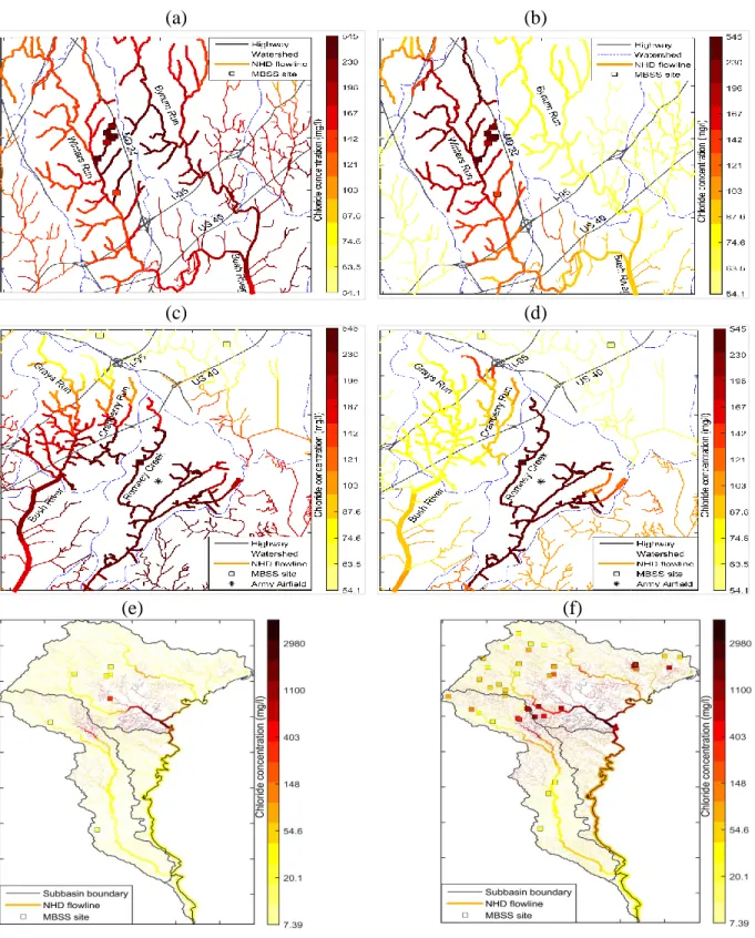
To the best of our knowledge, previous studies have not compared, and quantified, the difference in estimated levels obtained using an Euclidean versus river BME methods in that situation. To address this question, we provide here a comparison of the Euclidean versus river BME maps in area B and area C (figure 1 depicts where areas B and C are located). The purpose of this comparison is purely to emphasize the difference in chloride estimates using Euclidean versus river BME along unsampled river reaches. These maps are not meant to compare the estimation accuracy of the Euclidean and river BME methods at unsampled locations.
The Euclidean BME and river BME maps for area B are shown in figures 3(a) and 3(b), respectively. In that area we are interested in the assessment of Bynum Run, which lacks monitoring data, and runs parallel to Winters Run where monitoring data are available. Figures 3(a) and 3(b) show that in this area major highways (a known source of chloride) are aligned along the river network. The river distance between the monitoring stations on Winter Run and estimation points on Bynum Run are long, resulting in a low autocorrelation in chloride
37
defined by the U.S. EPA (U.S. Environmental Protection Agency. Ambient water quality criteria for chloride., 1988)), and 145 mg/l (a concentration level at which declines in survival of
salamanders have been documented (Stranko et al., 2013)). We find that according to Euclidean BME, 14% of Bynum Run river miles North of US 40 exceed 230 mg/l, and 62% of these river miles exceed 145 mg/l, whereas none of these river miles exceed either threshold limits
according to river BME.
38
(a) (b)
(c) (d)
(e) (f)
39
These results demonstrate that there can be big differences in the estimated chloride concentration using Euclidean BME and river BME, which may lead to substantial differences in the assessment of whether a river reach is impaired. For example using the Euclidean approach one might conclude that Bynum Run and the Grays and Cranberry Runs are in need of remedial action, while using the river approach one might conclude that remedial action is less needed and added monitoring is desired. The implication of this finding is that using the proper approach does matter, and therefore one should use the river BME approach introduced in this work rather than the classical Euclidean approach when estimating chloride along unmonitored river miles. Another implication of this finding is that using river BME, one will delineate impaired areas that are confined along river reaches, as opposed to spread isotropically across land, which may be easier to remediate because resources will be targeted to a specific subwatershed, rather than spread across multiple subwatersheds.
3.7. Space/time Patterns in Chloride Contamination
The rate of urban development, changes in road salt application practices, and changing climate conditions may drive a variety of spatial and temporal patterns in chloride concentrations (Corsi et al., 2015). Accurate estimation of chloride is crucial to understand these patterns, to improve our understanding of the extent and nature of chloride contamination, and to design effective measures to control the chloride pollution. A series of chloride concentration maps from 2005 to 2014 are constructed using the space/time river BME method introduced in this study. The maps obtained for 2014 are shown in figure 3, while maps for other years are in SI. These maps provide the first representation of chloride distribution that fully integrates