Tensor network representations
from the geometry of entangled states
Matthias Christandl1, Angelo Lucia1,2,3, P´eter Vrana1,4,5, Albert H. Werner1,2,*
1 QMATH, Department of Mathematical Sciences, University of Copenhagen, Universitetsparken 5, 2100 Copenhagen, Denmark
2 NBIA, Niels Bohr Institute, University of Copenhagen, Blegdamsvej 17, 2100 Copenhagen, Denmark
3 Walter Burke Institute for Theoretical Physics and Institute for Quantum Information & Matter, California Institute of Technology, Pasadena, CA 91125, USA
4 Department of Geometry, Budapest University of Technology and Economics, Egry J´ozsef u. 1., 1111 Budapest, Hungary
5 MTA-BME Lend¨ulet Quantum Information Theory Research Group * [email protected]
Abstract
Tensor networks provide descriptions of strongly correlated quantum systems based on an underlying entanglement structure given by a graph of entangled states along the edges that identify the indices of the local tensors to be con-tracted. Considering a more general setting, where entangled states on edges are replaced by multipartite entangled states on faces, allows us to employ the geometric properties of multipartite entanglement in order to obtain representa-tions in terms of superposirepresenta-tions of tensor networks states with smaller effective dimension, leading to computational savings.
Contents
1 Introduction 2
2 Matrix product states & Algebraic complexity theory 3
3 From PEPS to entanglement structures induced by hypergraphs 8
4 Exact state representations from degenerations 12
5 Plaquette conversions 15
5.1 From MaMuk(m) to GHZk(m): the casem= 3 15
5.2 From MaMuk(m) to GHZk(m): the general case 20
5.3 Bond dimension ofλis strictly larger than 2 22
6 Conclusions 25
A Computational complexity of tensor-contractions 27
A.1 Exact contraction of the RVB state on the kagome lattice 27
A.2 PEPS with varying bond dimension 28
A.3 Approximate contraction of the RVB state 30
References 32
1
Introduction
Taming the exponential growth of complexity with increasing system size presents one of the major problems in the theory of quantum many-body systems. Tailor-made Ansatz-classes such as tensor network states have allowed for tremendous progress over the last two decades both in terms of numerical [1–4] as well as analytical work [5, 6]. This includes results on ground state properties [7–9], the classification of quantum phases [10,11], disordered systems [12–16], the behaviour of open quantum many-body systems [17, 18], critical systems [19], as well as related to the AdS/CFT-correspondence [20].
At the heart of such tensor network approaches is the idea to obtain a class of physical states of interest from an underlying resource state by the application of local linear operations, which can be seen as applying stochastic local operations and classical communication [21]. In the case of matrix product states (MPS) and projected entangled pair states (PEPS) these states are given by networks of maximally entangled states. For certain applications, other tensor network structures have been introduced such as tree tensor networks [22, 23] and the multi-scale renormalization ansatz (MERA) [24, 25], the latter capturing ground state properties of critical systems.
Another route to generalizing MPS and PEPS, which has been recently explored, allows for more general resource states beyond EPR-pairs [26–28]. These are based on multi-partite quantum states shared among several lattice sites such as GHZ-states [27]. In this work, we further generalize this approach by extending both the underlying resource state or entan-glement structure as well as the class of allowed operations. More precisely, we allow for one-parameter families of approximate representations, which reproduce the state of interest to an arbitrary precision.
We show how these approximate representations can be turned into exact representations in terms of a moderate number of linear superposition of tensor network states. This approach provides more efficient tensor network representations for certain classes of states, and gives rise to an efficient algorithm to reconstruct expectation values faithfully. In addition, we obtain results that allow to simulate or re-express tensor network states based on multi-partite resource states in terms of ordinary PEPS, thereby enabling a numerical treatment of these states by the highly optimized methods that exist for PEPS. As a concrete example, we show that that semi-injective PEPS on the two-dimensional square lattice based on GHZ states as introduced in [27] with bond dimensionDcan be represented as a normal PEPS of bond dimension 2D.
As an example of the application of our results, we consider the Resonating Valence Bond (RVB) state, which has originally been proposed as the ground state of spin liquids [29] and is also of importance in the theory of high-temperature superconductivity [30]. The RVB
state has also been studied extensively in the context of PEPS [31–33]. A first tensor network representation of this state as a PEPS with bond dimension equal to 3 was introduced in [31]. We present two new representations of the state: a PEPS with non-uniform bond dimensions on the kagome lattice, with bonds of dimension (2,2,3) depending on the orientation of the bond, which we show is optimal; and a representation in terms of a superposition of a linear (in the system size) number of PEPS with bond dimension equal to 2.
The paper is organized as follows. In Section 2, we revisit the definition of MPS and connect it to notions in algebraic complexity theory. In particular, we introduce degenerations as a way of obtaining approximate state representations with smaller bond dimension. This leads to the concept of border bond dimension and we give a first example in terms of the W-state where this approximate representation leads to a provably more efficient representation. These ideas are then generalized in Section 3 to PEPS and other entanglement structures of multi-partite states, seen as representations of graphs and hypergraphs. In Section 4, we consider the question how to transform a given entanglement structure into another one based on degenerations and provide an efficient algorithm to compute exact expectation values even in this approximate setting. At the same time, this result lets us interpret states obtained from degenerations as arising from superpositions of tensor networks states with the number of superimposed states growing linearly with the system size.
The main building block for this general result turns out to be an approximate conversion between the plaquette states of the two entanglement structures involved. Therefore, we present in Section 5 specific examples of such plaquette conversions between important tensor network classes such as PEPS, generalized injective PEPS and the RVB state on the kagome lattice, proving lower and upper bounds on the required bond dimensions. In Appendix A we include an analysis of the computational cost of computing expectation values of tensor networks states on the square and kagome lattice using these more efficient approximate representations, focusing in particular on the RVB state.
2
Matrix product states & Algebraic complexity theory
As a starting point for more general tensor networks, we discuss in this section the concept of MPS representations from the point of view of algebraic complexity theory. In particular, we introduce the concept of degenerations, which correspond to a weaker notion of MPS representations that allows for a controlled approximation error. We then show that this notion leads to a more efficient translation-invariant MPS representation of the W-state on a ring.
Let us first recall the definition of an MPS. To this end, we consider a state vector T ∈ Cd⊗L
of L spins of local dimension d. Expanding T with respect to a product ba-sis{|i1, . . . , ili}we obtain T = d X i1,...,iL=1 Ti1,...,iL|i1, . . . , ili (1)
withTi1,...,iL denoting the basis coefficients. An MPS representation of T can now be seen as
a particular way of decomposing the orderL coefficient tensor Ti1,...,iL according to
Ti1,...,iL= tr Mi1[1]· · ·Mi[L] L (2)
Ti1,...,iL = ΩD1,2 ΩD2,3 ΩD3,4 A1 i1 A2 i2 A3 i3 A4 i4
Figure 1: Matrix product states as a network of maximally entangled states ΩD shared between physical sites of the 1D lattice to which local operationsAj are applied on combined
virtual space on each site.
with Mi[j]
j being a D×D-matrix of sufficiently large dimension D, the so-called bond
di-mension. For each spin j = 1, . . . , L, we can then define an order 3 tensor according to M[j]=Pd j=1 PD α,β=1(M [j] i )α,β|αihβ| ⊗ |ii and by setting Aj =Pdj=1PDα,β=1(Mi[j])|iihαβ|, we
can in turn express the state vector T as
T = L O j=1 Aj L O k=1 ΩDk,k+1 ! , ΩD = D X l=1 |l, li, (3)
which is an MPS representation with periodic boundary conditions and bond dimensionDof the stateT. Note that the two tensor products in (3) are shifted with respect to each other by half a physical lattice site such that Ωk,k+1 corresponds to a maximally entangled state shared between the lattice sites kand k+ 1, whereas Aj acts on the combined virtual space
CD⊗CD at lattice sitej (see also Figure 1). The important observation about (3) is the fact
that we are applying these linear mapsAj locally at each lattice site to an underlying resource
state, which in the case of an MPS is given by maximally entangled pair states ΩD shared
between neighbouring lattice sites if we think of theLspins positioned on a one-dimensional ring.
The question of whether a given vector ψ living in a tensor product spaceNL
j=1Cdj can be transformed into a stateφ∈NL
j=1C
d0
j via local linear mapsA
j :Cdj 7→ Cd
0
j is known in
the context of algebraic complexity theory as restriction.
Definition 1 (Restriction). Given ψ∈ Nm
j=1Cdj and φ∈
Nm
i=jC d0
j we say that ψ restricts
toφ, denoted as ψ≥φif there exist linear maps {Aj :Cdj 7→Cd
0 j} such that m O j=1 Aj ψ=φ . (4)
Note that the domain of the local mapsAj is implicitly specified via the chosen tensor
de-compositionNm
j=1Cdj of the underlying Hilbert space, i.e. eachAj acts on the corresponding
tensor factor in this decomposition.
An important generalization of the concept of restriction is that of degeneration. Here, instead of an exact conversion according to (4), we allow for approximate conversions between a stateψ to a state φby local operations.
Definition 2 (Degeneration). Let ψ ∈Nm
i=1Cdi and φ∈
Nm
i=1Cd 0
i be pure states. We say
Ai(ε) :Cdi 7→Cd
0
i, depending polynomially onε, such that
(A1(ε)⊗ · · · ⊗Am(ε))ψ=εdφ+ e
X
l=1
εd+lφel, (5)
for some tensorsφel and some integerd. We simply write ψDφifψDeφfor some error degree
e.
Remark 3. It is known (see e. g. [34]) that the definition of degeneration as given in (5) is equivalent to the following statement: ψDφif there exists a sequence(Aj(n))mj=1
n of linear mapsAi(n) :Cdi 7→Cd 0 i such that lim n→∞(A1(n)⊗ · · · ⊗Am(n))ψ=φ .
Remark 4. The notion of degeneration is strictly weaker than that of restriction, in that given two vectorsψ∈Nm
i=1Cdi,φ∈
Nm
i=1Cd 0
i,ψcan degenerate to φeven if we cannot find
a restriction, i. e. ψDφ, but ψ 6≥ φ. A well known example of this fact is the degeneration from the GHZ-state on three qubits to the W-state [21, 35, 36] (see also the W-state example at the end of this section)
Let us denote by GHZk(m) the k-level Greenberger–Horne–Zeilinger (GHZ) state on m
parties: GHZk(m) = k X i=1 |ii ⊗ · · · ⊗ |ii | {z } mtimes . (6)
We note that GHZkagrees with the unit tensor in algebraic complexity theory, usually denoted
ashki. In the cases when m is small, as in the case m = 3 which we will study extensively, we will use the following graphical notation to represent the GHZ state:
GHZk(3) = k
X
i=1
|ii |ii |ii= k .
When the number of parties is clear from the context, we will simply write GHZkfor simplicity.
Seen as the unit tensor, the GHZ state plays a special role in algebraic complexity theory, which leads us to define the following quantities.
Definition 5(Rank and border rank). Forφ∈Nm
i=1Cdi we define therank andborder rank ofφas
R(φ) = min{k∈N; GHZk(m)≥φ}, (7)
R(φ) = min{k∈N; GHZk(m)Dφ}, (8)
respectively.
Remark 6. Both the rank and the border rank depend on the tensor product structure of the space whereφlives: if we regroup the tensor product differently, the rank might change. It is easy to see that if we group factors together, i. e. we see φ not as an m-partite state but as an m0-partite state, with m0 < m, then both the rank and the border rank will not
increase. This is due to the fact that after regrouping the state GHZk(m) becomes the state
GHZk(m0), so if a restriction/degeneration to φ was possible before grouping it will still be
possible after grouping.
Moreover, if m = 2, then both rank and border rank of φ coincide with the Schmidt rank across the bipartition. Therefore, we can see that the maximal Schmidt rank across any possible bipartition,
Srmax(φ) = max
K⊂{1,...,m}rank trK|φihφ| , (9)
is a lower bound toR(φ).
The question whether a given quantum state φ can be represented as an MPS with periodic boundary conditions of bond dimension D is equivalent to the question, whether
NL
k=1ΩDk,k+1 ≥ φ, where ΩDk,k+1 again corresponds to a maximally entangled state with D levels shared between the physical lattice sites k and k+ 1 (see also Fig. 1). The state
NL
k=1ΩDk,k+1 is known in the context of algebraic complexity theory as the iterated matrix multiplication tensor, which is indeed the L-tensor given by maximally entangled states of dimensionsD1,D2,. . .,DLarranged in a cycle. We will denote this tensor as MaMuD1,...,DL
(for Matrix Multiplication):
MaMuD1,...,DL =
D1,...,DL X
i1,...,iL=1
|iLi1i ⊗ |i1i2i ⊗ · · · |iL−1iLi. (10)
This tensor is often denoted as hD1, . . . , Dmi in algebraic complexity. We write MaMuD(L)
ifD=D1 =· · ·=DL, a case typically denoted as IMMLD in the literature. As in the case of
the GHZ state, we will write MaMuk without the parameter mwhen this does not cause any
ambiguity.
In the cases whereL is fixed and small, as for example whenL= 3, we will use a similar graphical notation as for the GHZ-state:
MaMuD1,D2,D3 = D1,D2,D3 X i1,i2,i3=1 |i1, i2i |i2, i3i |i3, i1i= D1 D2 D3
As mentioned before, MaMuD(L) restricting to an L-tensor φ is equivalent to φ
admit-ting an MPS representation of bond dimensionD with periodic boundary conditions. More generally, since PEPS and other tensor network states are defined in terms of networks of maximally entangled states, we will be interested in conversions between MaMuK(L) and
other states. This leads us to define, in analogy to the rank and border rank the following quantities.
Definition 7 (Bond and border bond dimension). For φ ∈ Nm
i=1Cdi we define the (MPS) bond dimension and border bond dimension ofφas
bond(φ) = min{k∈N; MaMuk(m)≥φ}, (11)
bond(φ) = min{k∈N; MaMuk(m)Dφ}, (12)
Remark 8. Note that if we split the vertices{1, . . . , m}into{1, . . . , k}and{k+ 1, . . . , m}for somek= 1, . . . , m, and we see MaMuk(m) as a bipartite quantum state across this cut, the
resulting state is equivalent to MaMuk(2) = GHZk2(2) (since the MaMu tensor corresponds
to periodic boundary conditions). Similarly to (9), we can consider the maximal Schmidt rank across any cut instead of any bipartition (i. e. we only consider bipartitions where the two parts are contiguous in the spin chain):
Srcut(φ) = max
k∈{1...m}rank tr1,...,k|φihφ|. (13) Then by the previous argument, we see that
Srcut(φ)
1
2 ≤bond(φ)≤bond(φ).
To conclude this section, we present an example where degenerations offer a more efficient state representation, i. e. an example where we have a separation between bond and border bond dimension if we require a translation invariant representation in both cases. To this end, consider theW-state onL qubits defined as
W(L) = 1 X i1,...,iL=0 i1+···+iL=1 |i1, . . . , iLi . (14)
In the following, we give a translation-invariant representation of W(L) with border bond dimension 2 independent of the system sizeL. This representation follows immediately from the well-known fact that the W-state (viewed as a homogenous polynomialxL−1y) has border-Waring rank equal to two. For completeness we will give the argument below. In contrast to this border bond dimension 2 representation, the results from [37] on the quantum Wielandt inequality imply that the bond dimension of a translation-invariant restriction has to grow as exp 13ω(3L), withω(x) the product logarithm or Lambert function and it has been con-jectured that the growth should be of the orderL1/3 [6]. We note however that without the restriction to the translation invariant setting one can also find a bond dimension 2 represen-tation of the W-state.
In order to find a representation of the W-state W(L) on L parties with border bond dimension 2, note that
ψL(ε) = 1 0 0 ε ⊗L |0i⊗L= (|0i+ε|1i)⊗L=|0i⊗L+εW(L) +O(ε2) (15)
as a product state has bond dimension 1. Accordingly, the stateWf(ε, L) =ψL(ε)− |0i⊗Lis a
degeneration from MaMuL(2). The corresponding MPS-matrices of this translation-invariant
border bond dimension 2 representation can be chosen as
M0 = 1 0 0 (−1)1/L and M1= ε 0 0 0 , (16) because tr M0L= 0 and tr (M0nM1m) =εm.
3
From PEPS to entanglement structures induced by
hyper-graphs
Going beyond one spatial dimension, the procedure described for MPS can be generalized to higher dimensional lattices which leads to the notion of projected entangled pair states (PEPS) [2]. Again maximally entangled states are shared with neighbouring lattice sites, and the local operations preparing the state of interest from this underlying resource state are allowed to operate on the combined virtual space that includes all these subsystems. This motivates the following definition of tensor networks and entanglement structures for general graphs.
Definition 9(Entanglement Structure (Graph)). LetG= (V, E) be a graph with vertex set V, edge set E, and let w be an integer-valued weight function on the edge set w :E → N. For each e ∈ E, let Ωe ∈ Cw(e)⊗Cw(e) be the maximally entangled state of Schmidt rank
w(e). Anentanglement structure orcontraction scheme w.r.t. to Gis then given by
Ψ(G) =O e∈E Ωe∈ O v∈V CDv. (17)
with the local virtual dimension at vertexv∈V given byDv =Qe:v∈ew(e). We call thebond
dimension of Ψ the quantity maxv∈V{deg(v)
√
Dv}.
For a fixed integer D we will denote by ΨD(G) the entanglement structure obtained by
setting a constant weight w(e) =Don the graph (which will then have bond dimension D). We will also say that a stateφ∈N
v∈V Cdv is representable by Gwith bond dimension Diff
ΨD(G)≥φ, where the locality structure of the restriction mapsAj is given by vertex-setV
ofG according to the tensor decompositionN
v∈V CDv.
Remark 10. We remark that the term bond dimension is used in two different contexts. In Definition 9 it refers to the dimensionality of the maximally entangled states that form the graph entanglement structure, whereas in Definition 7 it characterizes for a given state vector the minimal bond dimension necessary to represent the state as an MPS. Note also that the notion of bond dimension and border bond dimension given in Definition 7 can be naturally extended to the case of entanglement structures defined on a general graph, i. e. as
bondG(φ) = min{D|ΨD(G)≥ψ},
and similarly for bondG. Since the tensor MaMuk(m) can also be written as Ψk(Cm), whereCm
is the cycle graph onm vertices, Definition 7 of bond dimension and border bond dimension coincide with bondCm and bondCm
Accordingly, MPS and PEPS fit naturally in this setting with the graph represented given by the path graphLL in the case of open boundary MPS, by the cycle graph CL in the case
of periodic boundary MPS, and by a lattice graph in the case of PEPS, respectively (see Figure 2). However, also more general tensor networks that allow for example for maximally entangled states between next-to-nearest neighbours can be captured within this framework. Definition 9 identifies the notion of representability again with the existence of a restriction according to Definition 1, where the linear maps{Ai}correspond to the local tensors defining
the tensor network state. We remark that our notion of bond dimension is chosen in such a way that it captures how the number of parameters necessary to specify such a tensor network
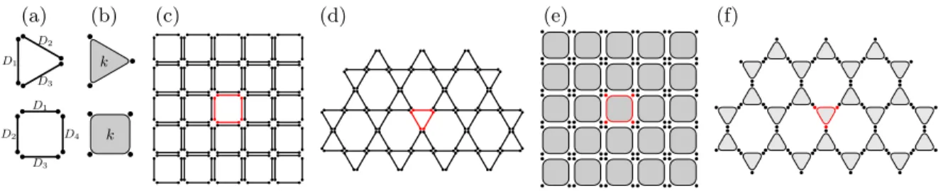
(a) D1 D2 D3 D1 D3 D2 D4 (b) k k (c) (d) (e) (f)
Figure 2: Examples of entanglement structures: (a) Plaquette tensors given by maximally entangled states shared cyclically between three and four sites, where the indices Di denote
the number of levels of the entangled states; (b) same as in (a) but with a GHZ-state of k levels shared between the sites; (c-d) entanglement structures on the square and kagome lattice, the plaquette shown in red indicates how to obtain those from the plaquette states from (a), neighbouring entangled states on the same edge can be reinterpreted as a single maximally entangled state with the number of levels squared; (e-f) same lattices as in (c-d) but with a generalized PEPS based on 3- and 4-party GHZ-states.
state scales with the system size. More precisely, given the bond dimension D, the number of parameters scales as O(|V|Ddeg(G)dmax), where dmax is the maximal physical dimension given by maxi∈V(di) and deg(G) is the maximal degree of the vertices ofG. This definition is
general enough to capture savings in the bond dimension due to non-uniform edge dimensions with respect to the different edges in the graph, but at the same time reduces to the usual scaling ofO(|V|D2dmax) or O(|V|D4dmax) in the case of MPS or PEPS with uniform bond dimension, respectively.
We will now generalize the concept of contraction schemes to representations of hyper-graphs, where the underlying entanglement structure is given by multipartite entangled states shared among all vertices that are connected by a hyperedge.
Definition 11 (Entanglement Structure (Hypergraph)). Let G = (V, E) be a hypergraph, with vertex-setV and hyperedge setE. For eache∈E, let Ωe∈Nv∈eCDv,e be a pure state.
Anentanglement structure orcontraction scheme w.r.t. toG is then given by
Ψ(G) =O e∈E Ωe∈ O v∈V CDv.
with the local virtual dimension at vertex v ∈ V given by Dv = Qe:v∈eDv,e and the bond
dimension of Ψ(G) defined asD= maxv∈V{ deg(v√)
D}.
Note that, contrary to the graph case, the hypergraph entanglement structure is not simply defined by weights on the hyperedges but also by the choice of multi-partite entangled states Ωe (since there exist non-equivalent multi-partite entangled states, we cannot simply specify
the edge dimension as in the case of graphs). As an example, note that the GHZk(m) can
be written as an entanglement structure on the hypergraphHm with m vertices and a single hyperedge containing all vertices:
V(Hm) ={0, . . . , m−1}, E(Hm) ={V},
In analogy to the graph case, we can still consider a hypergraph entanglement structure Ψ(G) as a contraction scheme, with a state φ being representable by Ψ(G) iff we can find local maps{Av :CDv 7→dv}satisfying (4) (i. e. iff Ψ(G)≥φ). Note that as in the graph case,
the locality structure of the restriction maps Aj is given by vertex-set V of G according to
the tensor decompositionN
v∈V CDv.
Particular examples of entanglement structures on hypergraphs from the literature are projected entangled simplex states [28] and semi-injective PEPS [27]. In the latter case, the vertex set is given by the same vertices of the two-dimensional square lattice on L×L sites (i. e. CL×CL), but instead of having an edge for each pair of neighbouring sites, there is instead an hyperedge containing the 4 vertices in each of the plaquettes:
V = [0, L]×[0, L]∩Z2,
e∈E ⇐⇒ e={(i, j),(i+ 1, j),(i, j+ 1),(i+ 1, j+ 1)} for some (i, j)∈V.
Finally, for each hyperedgee, we choose a GHZ state on 4 parties as Ωe, so that the resulting
entanglement structure is given by
Φ =O
e∈E
GHZk(4).
The bond dimension of Φ is then simply given by the number of GHZ levels k. For k = 2 this class of states also includes the ground state of the CZX-model, exhibiting an on-siteZ2 symmetry [26].
In order to find representations of physical states with optimal bond dimension, we will analyze how well a given contraction scheme can be expressed in terms of another. To this end, we introduce the following definition, which specializes Definition 1 to the particular case of entanglement structures.
Definition 12 (Conversion of entanglement structures). Let G and G0 be two graphs or hypergraphs with the same vertex setV. Given two entanglement structures Ψ(G) and Ψ(G0) we say that Ψ(G) restricts to Ψ(G0), and we write Ψ(G) ≥Ψ(G0), if there exist linear maps Av :CDv →CD
0
v for each v∈V such that
O
v∈V
Av
!
Ψ(G) = Ψ(G0), (18)
whereDv and D0v are the local dimension at vertexv of Ψ(G) and Ψ(G0), respectively. The
notion of degeneration specializes to the case of entanglement structures exactly in the same way as restrictions (i. e. by allowing local maps to act according to the tensor product structure defined by the vertex setV).
Remark 13. Note that in the case of a path graph LLon Lsites and a graph entanglement
structure Ψk(LL) (i. e. the entanglement structure of an open boundary condition MPS of
bond dimension k), the existence of a degeneration implies the existence of a restriction. More concretely, if Ψk(LL)DT for some L-partite quantum state T, then also Ψk(LL)≥T.
This is due to the fact that, by sequential SVD decompositions (see [6, Theorem 1] and [4, pag. 18-20]), it is possible to construct T with a bond dimension equal to the maximal Schmidt rank across any cut Srcut(T) (see (13)): equivalently Ψk(LL) ≥T for k= Srcut(T). On the other hand we can repeat the argument of Remark 8 for Ψk(LL), but taking into account
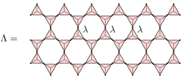
Λ = λ λ λ
Figure 3: The hypergraph entanglement structure Λ of the RVB state. The triangles represent theλtensor, and the entanglement structure Λ is obtained by tensoring 23L copies of it and arranging the vertices according to the kagome lattice.
that we have open boundary conditions instead: we see that after grouping neighbouring sites we can convert Ψk(LL) to Ψk(LL0) withL0 < L, so that if Ψk(LL)DT then necessarily k ≥ Srcut(T). On the other hand, as soon as there are cycles in the graph, this argument breaks down, and we have already seen in the W-state example at the end of Section 2 that a degeneration can exist when the corresponding restriction does not.
RVB state Another example of entanglement structure is found in the context of PEPS representations of the Resonating Valence Bond state (RVB) [31–33]. Rephrasing the con-struction used in [32] in terms of Definition 11, the RVB state on the kagome lattice can be represented by an entanglement structure Λ, where we assign to each plaquette the 3-party entangled stateλ∈(C3)⊗3 (see Figure 3) given by
λ= 2
X
i,j,k=0
i,j,k|i, j, ki+|2,2,2i= , (19)
wherei,j,k denotes the antisymmetric tensor with0,1,2= 1.
In [32] the entanglement structure Λ for the RVB state composed of plaquette tensors λ was shown to have a PEPS representation with bond dimension 3, by constructing the explicit linear maps realizing the conversion. The RVB state on the kagome lattice thus has bond dimension at most 3. We now give a representation of the same state with border bond dimension equal to 2 (in other words we reduce the local virtual dimension at each vertex from 34= 81 to 24 = 16), which, as we show in Section 5.3, is smaller than the optimal PEPS representation that can be obtained with restrictions.
In order to do so, we need to show that 2 2
2 D . The MPS matrices of the degeneration are given by M0[j]() = 1 2 0 0 , M1[j]() = 0 − 0 , M2[j]() = 1 0 0 −1 +δj,3 2 2 1 0 0 1 (20)
withj= 1,2,3, resulting in the state ε2λ+ε4|2i ⊗(14|00i − |11i).
In the following section, we will show how this improved representation can be used to compute exact contractions and expectation values for the RVB state.
4
Exact state representations from degenerations
Having introduced the concept of tensor network representations in terms of degenerations and border bond dimension in the previous sections, we will now turn to the question how to obtain physical information in this approximate setting. To this end, we present a general method to turn an approximate conversion between two entanglement structures given by degenerations into an exact one by allowing for superpositions. The main advantage of this approach is on the one hand that this can be accomplished with only a linear overhead in the number of plaquette states involved and on the other hand that it also allows for the computation of exact expectation values. These properties are summarized in the following theorem. The proof relies on results from algebraic complexity theory [38, 39] and we include the argument here for the sake of completeness.
Theorem 14. Let Ψ and Φ be the entanglement structures obtained by placing ψ and φ,
respectively, on F faces of a lattice with L sites. Assume T can be represented by Φ, i. e.
Φ≥T. If ψDφ, then T = eF X i=0 Wi, (21)
where eachWi can be represented by Ψ, i. e.Ψ≥Wi. The number of terms in the
representa-tion is linear inF, i. e. the constanteis only dependent on the degenerationψDφ. Moreover
expectation values of an observable O under T can be computed from expectation values of
2eF + 1states represented by Ψ:
hT, OTi= 2eF
X
i=0
γihVi, OVii, (22)
where again eachVi can be represented byΨ, i.e. Ψ≥Vi ∀i, andγi∈Rare known constants
depending onVi.
Proof. According to Definition 2,ψDφif there exist linear mapsAi() :Cdi 7→Cd
0
i, depending
polynomially on the parameter, such that
(A1()⊗ · · · ⊗Am())ψ=εdφ+ e
X
l=1
d+lφel,
for some multi-partite statesφel, approximation degree dand error degreee. We observe that
the plaquette degeneration φDψ immediately implies that φ⊗F Dψ⊗F, as can be seen by taking the tensor product of the local operators given by the degeneration φDψ. As was already observed in [39, Prop. 4], the error degree will only grow linearly in the number of copies of the degeneration maps, i. e. the number of faces F in the lattice and therefore we see that the product ofF copies of φdegenerates toF copies of ψwith error degree eF:
ψ⊗ψ⊗ · · · ⊗ψ
| {z }
F copies
DeFϕ⊗ϕ⊗ · · · ⊗ϕ. (23) This degeneration is possible, when all m parties of each of the F copies are considered independently, i. e. when the states in (23) are regarded aremF-partite states. In [39] this was
a) A(ε)
B(ε)
C(ε) =⇒ D
b)PeFi=0γi
A(εi)
B(εi)
C(εi)
=
Figure 4: Graphical representation of Theorem 14: a) A local degeneration (A(ε),B(ε),C(ε)) depending polynomially on ε from one plaquette state (pairwise entangled states between three parties) to another (λ state), gives rise to a global degeneration between a collection of F plaquette states. b) Evaluating the degeneration at eF + 1 points εi, we can express
the full entanglement structure built from the second plaquette state (here λ states) as a superposition ofeF + 1 states that arise as restrictions from the first entanglement structure (here pairwise entangled states between three parties). The parameter e is a scaling factor depending on the polynomial degree of the local degeneration, the prefactorγi is obtained by
evaluating theith Lagrange polynomial `i at 0.
derived in order to show that tensor rank is strictly submultiplicative under the tensor product. Note that the degeneration resulting from grouping all theF copies of ψ and φ into an m-tensor was already considered in [38], and led to faster algorithms for matrix multiplication. In order to prove the theorem, we will consider instead a different consequence of this argument: grouping the mF tensor factors according to the underlying lattice, we obtain Ψ and Φ as L-partite states respectively, which means that
ψDeφ =⇒ ΨDeF Φ. (24)
Similar as in [38,39], we now apply Lagrange interpolation [40, p. 260] in order to transform the degeneration into a restriction. From (24), we can write
F O i=1 m O l=1 Al(ε) !! Ψ =εdΦ + eF X k=1 εd+kΦek (25)
for some integerd, where the linear maps Al(ε), depending polynomially on ε, are given by
copies of the degeneration maps of ψDφ corresponding to the plaquettes f = 1, . . . , F. Let (Bl)l be the local operators given by the restriction Φ≥T at the lattice sites l= 1, . . . L, i. e.
NL
i=1Bl
Φ =T. Composing (24) with the (Bl)l and dividing by d, we define
T() =−d L O i=1 Bl ! F O i=1 m O l=1 Al(ε) !! Ψ =T + eF X k=1 εkTek. (26)
Considering the right hand side, we immediately see that T() depends polynomially on with degree eF, and that T(0) = T. Moreover, for each 6= 0, T() is a restriction from Ψ. EvaluatingT() at eF + 1 points (i)eFi=0, we can obtain the value at= 0 via Lagrange
interpolation: T =T(0) = eF X i=0 γiT(i),
where γi = `i(0) is obtained by evaluating the ith Lagrange polynomial `i at 0. Defining
Wi =γiT(i), we obtain (21). In order to prove (22), we observe that any expectation value
with respect toT() is given by
hT(), OT()i=hT, OTi+ eF X k=1 D T, OT˜k E εk+DT˜k, OT E ()k+ eF X k,k0=1 D ˜ Tk0, OT˜k E ()kεk0. (27)
In caseε∈Rthis is again a polynomial inεnow of degree 2eF. Similarly as before, computing
hT(), OT()i for a fixed ∈R amounts to computing an expectation value for a state T() which has a representation in terms of Ψ. Computing 2eF + 1 of such expectations values is then again sufficient for computing hT(), OT()i at = 0 via interpolation, this proves (22).
Let us note that we are not limited to useε∈R, but can also chooseε∈Cif that is more convenient. To this end, let us consider the expression
hT(ε), OT(ε)i=hT, OTi+ eF X k=1 D T, OT˜k E +DT˜k, OT E εk+ eF X k,k0=1 D ˜ Tk0, OT˜k E εk0+k.
This is by design again a 2F degree polynomial in ε with the expectation value hT, OTi
in leading order. Hence, computing the scalar product hT(εi), OT(εi)i for 2F + 1 different
values ofεi will again allow us to compute the value of this polynomial at ε= 0 and therefore
hT, OTi. Alternatively, we could also just insert ε directly into (27) and treat Re(ε) and Im(ε) as independent variables.
We also note that the due to the reduced bond dimension for each of theVi also the error
caused by approximate contraction will be smaller and that by oversampling the number of evaluation points in the degeneration, there is an additional potential for improving the accuracy of the contraction.
Theorem 14 provides degenerations that transform the two entanglement structures into each other plaquette by plaquette. Constructions based on larger units (e.g. several plaque-ttes) might lead to further reductions in the bond dimension, since the maps on the vertices that are grouped together no longer have a tensor product constraint.
Before looking more generally on plaquette conversions between important classes of tensor networks in the next section, as a first application of the theorem we come back to the RVB state on the kagome lattice in terms of the Λ entanglement structure introduced at the end of section 3. We have presented a degeneration from 2
2
2 to the plaquette tensors of Λ,
which has approximation degreedand error degree eboth equal to 2. Rolling this out on the kagome lattice with F triangles, we obtain a border PEPS representation of the RVB state of border bond dimension 2 and Theorem 14 then ensures that we can reconstruct the RVB state as a superposition of 2F+ 1 PEPS of bond dimension 2 or compute expectation values with 4F+ 1 contractions.
5
Plaquette conversions
In this section, we present general strategies and examples for optimized conversion between plaquette states in terms of degenerations. To this end, we consider m-tensors, i. e. elements ofNm
i=1Cdi, for some non-zero integers (di)i, which can be equivalently seen as unnormalized
purem-partite quantum states. We will usually considermto be a small integer (oftenmwill be equal to 3 or 4), as thesem-tensors are the building blocks of the entanglement structures we considered in Section 3. After some definitions and examples that set the scene, we will study the conversion between maximally entangled states shared around circles and GHZ states, which are the basis for conversion between PEPS and more general tensor network states. To do this, we utilize the correspondence between entangled pairs on the circle and the matrix multiplication tensor (see e.g. [41]). This will be first done for 3-party tensors and subsequently for tensors ofm parties. In addition, we prove in Section 5.3 that the MPS representation with bond dimension (2,2,3) for the state λ, which is the basis for the PEPS representation of the RVB state, is optimal.
5.1 From MaMuk(m) to GHZk(m): the case m= 3
The aim of this section is to investigate restrictions and degenerations from MaMuk1,k2,k3 to
GHZk(3) and viceversa: this will allow us the express GHZ based hypergraph entanglement
structures on triangular lattices as bond and border bond PEPS representations. In particular, we will prove the following proposition.
Proposition 15. 1 2 1 +√4k−3 <bond(GHZk(3))≤ O k 1 2+ c √ logk , (28)
for some fixed positivec. In other words,
MaMun(3)6≥GHZn2−n+1(3) and MaMun(3)≥GHZf(n)(3) (29)
where f(n) =O (n2)1− c0 √ logn
for some positive constant c0.
However, as it was shown by Strassen in [42, Thm. 6.6], there exist degenerations which allow for an MPS representation of GHZd3
4n2e(3) with border bond dimension n. Setting
n= 2, this shows in particular, that
2
2
2
6≥3
but2
2
2
D3
.Hence, bond(GHZ3(3))>2, whereas bond(GHZ3(3)) = 2.
Before giving the proof, we discuss a non-symmetric extension of this result, i.e. degener-ations from MaMuk1,k2,k3 with different values of k1, k2,k3. Following [43], we consider the
local diagonal operator
depending on an integerg which we will fix later. This leads to the transformation
(A(ε)⊗A(ε)⊗A(ε)) MaMuk1,k2,k3 =2g 2
k1,k2,k3
X
i1,i2,i3=1
(i1+i2+i3−g)2|i1, i2,i |i2, i3i |i3, i1i
=2g2
k1,k2,k3
X
i1,i2,i3=1
i1+i2+i3=g
|i1, i2i |i2, i3i |i3, i1i+O2g2+1
.
The leading order term in corresponds to a GHZ state, because fixing any pair of i1, i2, i3 determines the third one uniquely. Hence, we only have to determine the number of solutions to the equation i1+i2+i3 =g for given ni and inhomogeneity g. Choosing k1 = 2,k3 = 3 andk2 = 2 ork2 = 3 andg= 5 then directly leads to
2
2
3
D4
and2
3
3
D5
.These degenerations are optimal, both in the sense that the corresponding restrictions are not possible, and in the sense that we cannot obtain GHZ states with more levels from a degeneration of these MaMu tensors. It is also not possible to obtain the same GHZ states from MaMu tensors, where one of the bond dimension is smaller than the ones we have considered.
We will now turn to the proof of Proposition 15. We will first introduce two definitions and prove a lemma.
Definition 16. LetG= (V, E) be a graph. Anorthogonal representation of Gis a mapping
π:V → H \ {0},
from the graph into some inner product vector spaceH such that
(u, v)∈E =⇒ hπ(u)|π(v)iH= 0.
We will denote by dimH the dimension of the orthogonal representation.
Definition 17. LetKn,n be the complete bipartite graph on 2nvertices, i. e.
V(Kn,n) ={b0, . . . , bn−1, c0, . . . , cn−1}, E(Kn,n) ={(bj, ck)|j, k= 0, . . . , n−1}.
LetK0n,n be the graph obtained by removing the edge (b0, c0) from Kn,n:
E(K0n,n) =E(Kn,n)\ {(b0, c0)}={(bj, ck)|j, k= 0, . . . , n−1, j6=korj=k6= 0}. Lemma 18. With the notation defined above, let π:K0n,n → H be an orthogonal
representa-tion such thatdimH ≤2(n−1). Then at least one of the following holds
1. dim span{π(bi)|i= 1, . . . , n−1}< n−1,
3. π(b0) is orthogonal to π(c0).
Proof. Let B = span{π(bi)|i = 1, . . . , n−1} and C = span{π(ci)|i = 1, . . . , n−1}. Since
π(bi) is orthogonal to π(cj) for every i, j = 1, . . . , n−1, we have that B ⊥ C. If B ⊕ C is
not equal to H, which has dimension ≤ 2(n−1), then at least one of the two has to have dimension strictly smaller than n−1, so that either 1. or2. holds. If not, thenH=B ⊕ C. Sinceπ(b0) is orthogonal to everyπ(ci) fori= 1, . . . , n−1, it is orthogonal toC, and therefore
π(b0) ∈ B. Similarly, π(c0) is orthogonal to B and therefore lies in C. But then π(b0) and π(c0) live in orthogonal subspaces and they are themselves orthogonal.
We are now ready to prove Proposition 15.
Proof (Proposition 15). We will start by proving the lower bound of (28) as well as first part
of (29), since they are equivalent as can be seen by setting k =n2−n+ 1. Let us assume that GHZn2−n+1 has an MPS representation with bond dimension D ≤ n, and let us show
how to derive a contradiction from this fact. To fix notation, let
GHZn2−n+1 = n2−n
X
i,j,k=0
tr[AiBjCk]|i, j, ki,
for some non-zero matrices{Ai}i,{Bj}j and {Ck}k of dimensionD×D, such that
trAiBjCk=
(
1 if i=j =k, 0 otherwise.
We start by showing that ifD≤nwe can without loss of generality assume thatA0is non-singular. To derive this, we will use the following fact: any linear subspace ofMD containing
only singular matrices has dimension at most D2 −D [44]. Consider S = span{Ai|i =
0, . . . , n2 −n} ⊂ MD. S is the span of n2−n+ 1 matrices: if it contains only singular matrices, then its dimension can be at most D2−D. So if D ≤n, either in S there is one matrix which has full rank or dimS ≤ D2 −D ≤ n2−n, which implies that the matrices (Ai)i are not linearly independent.
LetW = (wij)∈U(n2−n+1) a unitary matrix such thatPn 2−n
i=0 w0iAiis either zero or full
rank. Then by denotingφi=W|iithe rotated basis, we see that (W⊗W⊗W) GHZn2−n+1 =
P
iφi⊗φi⊗φi has an MPS representation with matrices
˜ Ai = X j wi,jAj, B˜i = X j wi,jBj, C˜i = X j wi,jCj,
and ˜A0 is either zero or full-rank. The first case we can exclude, because tr ˜A0B˜0C˜0 = 1. This shows that up to a local unitary on the physical level, we can assume without loss of generality that A0 is not singular.
Let A0 =UΣV∗ be the singular-value decomposition of A0. Then Σ >0 defines a scalar product onMD 'CD
2
byhX|YiΣ= tr ΣX∗Y. Defining
we obtain an orthogonal representation of the graphK0n2−n+1,n2−n+1 (defined in Lemma 18)
onMD with inner producth·|·iΣ, since
hπ(bj)|π(ck)iΣ = tr ΣV∗BjCkU = trA0BjCk =
(
1 if j =k= 0, 0 otherwise.
IfD≤n, then dimMD =D2 ≤n2 < n2+ (n−1)2+ 1 = 2(n2−n+ 1), which implies that we can apply Lemma 18 and at least one of the conditions stated in it must hold true. If1.
or2. hold, then either span{Bi}or span{Ci}has dimension strictly smaller than n2−n+ 1,
but we have already seen that this leads to a contradiction. Therefore3. must hold, but this also leads to a contradiction: on the one hand we have proven that trA0B0C0 = 0 but we also know that know that trA0B0C0=hπ(b0)|π(c0)i= 1.
We will now prove the upper bound of (28). Our starting point is the following result [42, Thm. 6.6]
MaMunDγn 2
GHZd3n2/4e, (31)
for some constant γ > 0. Let α an integer to be determined later, and consider the tensor product ofα copies of (31). To simplify notation, we setk= (d3
4n
2e)α, so that we get
MaMunαDαγn
2
GHZk.
As we have discussed previously, it is a well known result in algebraic complexity theory that a degeneration can be turned into a restriction by interpolation paying a price in terms of a direct sum (see e.g. [34]). In the present context, this means that we can turn the degeneration into a restriction by supplementing a GHZ state with a number of levels equal to the error degree plus one (see e.g. [39]). Therefore we obtain
GHZαγn2+1⊗MaMunα ≥GHZk,
from which follows that
bond(GHZk)≤nαbond(GHZαγn2+1).
We can trivially bound bond(GHZαγn2+1) by 2αγn2,
bond(GHZk)≤2αγnα+2. (32)
From the definition of k, we haven≤ 4312
k21α, and by inserting this into the right-hand side
of (32), we obtain: bond(GHZk)≤2γα 4 3 1+α2 k12+ 1 α. (33)
We now want to chooseαin order to minimize the right hand side. We will instead simply minimize 43α2
k1α, as this will already give the right asymptotic scaling. Since the function
diverges to infinity when α tends to zero or to infinity, we find the minimum by setting the derivative of α2 log 43+ 1αlogk to zero:
1 2log 4 3 − 1 α2 logk= 0 ⇐⇒ α=α ∗= √ 2 log1/2(4/3)log 1/2(k)
Takingα=bα∗c, we obtain bond(GHZk)≤ 8 3 √ 2 log1/2(4/3)γk 1 2+ √ 2 log1/2(4/3) log1/2k + log logk 2 logk . (34)
Since log1/2(k) ≥ log logk, we can find c positive as claimed in (28). We can improve this bound by minimizing the right hand side of (33) instead, obtaining
bond(GHZk)≤ 8γ 3 log(4/3)k 1 2+ r 1+2 log(43)log(k) log(k) + log −1+ r 1+2 log(43)log(k) log(k) = 8γ 3 log(4/3)k 1 2e √ 1+2 log(4/3) log(k)(−1 +p 1 + 2 log(4/3) log(k))
Note that the asymptotic scaling of this bound is the same as the one we had obtained by minimizing 43
α
2kα1, as we claimed.
To get the second part of (29), let instead
m=αnα+2 ≤α 4 3 1+α2 kα2+2α , so thatk≥ 4 3 −α m α 2α
α+2. Then (32) implies for any α≥1 that
MaMu2γm ≥GHZ (4 3) −α (m α) 2α α+2 .
Ideally, we would like to take the maximum over α to obtain the best lower bound. Instead, we decide here to maximize the easier function
−αlog(4/3) + 2α
α+ 2logm,
neglecting the additional summand depending on−logα, since this will already be sufficient to get the desired scaling. The maximum is attained atα satisfying
−log(4/3) + 4 logm
(α+ 2)2 = 0 ⇐⇒ α=α
∗∗= 2 log1/2m log1/2(4/3)−2,
again since the function is smaller or equal to zero forα equal to zero or tending to infinity. Since both (4/3)−α and (m/α)α2+2α are decreasing inα, substitutingα=bα∗∗c, we obtain that
4 3 −α ≤ 4 3 2 (m2)− log1/2(4/3) log1/2(m) , and m α 2α α+2 ≤(m2) 1−log1/2(4/3) log1/2(m) h 1+log1m(log(2)−1 2log log(4/3)+ 1 2log logm) i which implies MaMu2γm≥GHZq with q=c(m2) 1−2log1/2(4/3) log1/2m , (35)
5.2 From MaMuk(m) to GHZk(m): the general case
In this section, we will outline a method to obtain explicit degenerations from MaMuk(m) to
GHZk(m), generalizing some of the results for the 3-party case from the previous section to
m parties. We will then work out in detail the case form = 4 as an example. We leave the reverse bound as an open problem.
As before, MaMuk(m) will denote a network ofmparties arranged on a circle each sharing
a maximally entangled state withk levels with each of its two nearest neighbours. The goal is to find a local linear transformation Al(ε) at each vertex l depending polynomially on ε
such that the leading contribution inεof the resulting state is anm-party GHZ state withk0 levels m O l=1 Al() ! k X i1,...,im=1 |i1i2i |i2i3i. . .|imi1i=d GHZk0(m) +O d+1
wherek0should be as large as possible and the kets indicate the grouping of parties. Following [43], we choose the operators Al() diagonal in the local product basis, i.e. Al(ε)|i, ji =
εpl(i,j)|i, ji. In addition, we require that the leading order contribution in εis given by those
vectors |i1, i2i · · · |im, i1i, that satisfy a certain system of linear equations, i. e. Plclil = g
with coefficients vectorcl and inhomogeneity g belonging toZν for some integer ν [43]. This
last condition is equivalent to the requirement that the vectorP
lclil−g is the zero vector,
which can be reexpressed by the norm condition
0 = * X l clil−g X l clil−g + = m X l=0 hcl|clii2l −(hg|cli+hcl|gi)il +hg|gi+X l6=l0 hcl|cl0iilil0. (36)
However, we have to connect this expression back to the local operationsAl(ε). Indeed, we
have to ensure that (36) can be generated by a product of local degenerations of the form
Al()|iji=pl(i,j)|iji ,
namely P
lpl(il, il+1) = d+k
P
lclil−gk22, which can always be achieved for all the terms in (36) that depend at most on a single indexl. However, for the cross-terms this requires
hcl|cl0i= 0 if|l−l0|>1, forcing the vectors cl into an orthogonal representation of the cycle graph (giving a lower bound onν), in which case we obtain
m O l=1 Al() ! k X i1,...,im=1 |i1i2i |i2i3i. . .|imi1i= k X i1,...,im=1 hPlclil−g|Plclil−gi |i1i2i |i2i3i. . .|i mi1i . (37)
Furthermore, we have to ensure that the leading contribution, given by
m X i1,...im=1 P lclil=g |i1, i2i · · · |im, i1i (38)
is indeed locally unitarily equivalent to a GHZ state, i. e. consists of an equal weight super-position of product states ψr = ψr,1 ⊗ · · · ⊗ψr,m, such that
ψr,l
is a superposition of vectors of the form |i1, i2i · · · |im, i1i this means that fixing a pair of indicesil0, il0+1 at any vertex l the linear equationP
lclil =g must have at most one unique
solution in the remainingil. One way of ensuring this is to choose the vectors cl,cl0 linearly independent, whenever|l−l0|>1. In other words, we have to choose the vectors (cl)l in such
a way that if we remove any subset of vectors that share a vertex, the remaining ones have to be linearly independent. The maximal dimension of the GHZ state we can extract is then given by the number of integer solutions to the equation
m
X
l=0
clil=g , (39)
where we optimize over the inhomogeneityg. One can get a bound on the number of these solutions by a probabilistic argument with respect to the inhomogeneityg.However, in order to talk about the finitem case, we are going write down an explicit expression for (39) that satisfies all the necessary properties, i. e.hcl|cl0i= 0 forl0 ∈ {/ l−1, l, l+1}and{cl}m
l=0\{cj, cj+1} linearly independent for allj. We define the equations inductively starting from the four-party case 1 1 i1+ −1 0 i2+ 1 −1 i3+ 0 1 i4 =g (40)
Now adding a new vertex and edge into the cycle betweeni4 and i1 means that now c4 has to be orthogonal to c1 and the new c5 should be orthogonal to all vectors exceptc1 and c4. This can be achieved by the choice
1 1 1 i1+ −1 0 0 i2+ 1 −1 0 i3+ 0 1 −1 i4+ 0 0 1 i5 =g . (41)
This procedure can be repeated leading to the following linear system for thek-cycle
1 −1 1 0 0 · · · 0 0 1 0 −1 1 0 0 0 1 0 0 −1 1 0 1 0 0 0 −1 .. . ... ... ... ... ... ... 1 0 0 0 0 1 0 1 0 0 0 0 −1 1 ·~i=g . (42)
In order to find the integer solutions to this problem, we employ the Smith normal form of the matrix on the left-hand side, which gives the general solution vector
~i= z1+z2+A1 (m−2)(z1−z2) +z2+A2 (m−3)(z1−z2) +z2 .. . 2(z1−z2) +z2+Am−2 z1 z2 , (43)
where z1, z2 are arbitrary integers and the constants (Al) depend on the choice of g by a
simple linear integer transformation given by the Smith normal form. In order to obtain the relevant solutions for our specific problem, we have to impose the upper and lower bounds 0 andk−1 if the original maximally entangled states are of dimensionk for each entry of the solution vector~i.
The case m= 4 In the casem= 4, (43) leads to the inequalities
0≤ z1+z2+g2 2z1−z2+g2−g1 z1 z2 ≤n−1.
Choosingg2 =g1 ∈ {k2,k−21}depending on whetherkis even or odd leads to the lower bound on the number of solutions of the form k22+1 for odd dimensions and k22 for evenk.
This shows MaMuk(4)DGHZdk2
2 e
(4), i. e. that we can locally degenerate from a cycle of four maximally entangled states withklevels to a four party GHZ state ofdk2
2elevels. Hence on the level of plaquette states, we can degenerate from pairwise maximally entangled states on four parties with d√2De levels to a GHZ state on four parties of D levels. Taking into account that in a two-dimensional square lattice the bond dimension of neighbouring plaquette states have to be combined (see Figure 2 (c) and (e)), this means that semi-injective PEPS on the two-dimensional square lattice based on GHZ states as introduced in [27] with bond dimensionDcan be represented as a normal PEPS of bond dimension 2D. By our theorem, expectation values for these generalized PEPS can hence be computed from expectation values of normal PEPS, for which highly optimized numerical codes exist.
5.3 Bond dimension of λ is strictly larger than 2
As discussed in Section 3, in [32] the PEPS representation of the RVB-state is obtained via the multipartite entangled state
λ= 2
X
i,j,k=0
εi,j,k|i, j, ki+|2,2,2i= , (44)
withεdenoting the completely antisymmetric tensor such that0,1,2= 1. In [32], the state λ was obtained as a restriction from 3
3
3, obtaining the same PEPS representation of the RVB
state with bond dimension 3 from [31]. It turns out that is sub-optimal: the tensorλcan be obtained also as a restriction from 3
2
2, using the following MPS representation:
M0[1] = 1 2 0 1 0 1 0 0 M1[1] = 0 −1 0 1 0 0 M2[1] = 1 0 1 0 −1 0 (45) M0[2] = 1 2 0 1 1 0 0 0 M [2] 1 = 0 −1 1 0 0 0 M [2] 2 = 1 0 0 −1 1 0 (46) M0[3] = 1 2 0 1 1 0 M1[3] = 0 −1 1 0 M2[3] = 1 0 0 −1 . (47)
This leads to a PEPS representation of the RVB state where the bond dimension is reduced from 3 to 2 on two of the edges of each triangle of the kagome lattice.
We now prove that this representation is optimal, i. e. that λ cannot represented as an MPS of bond dimension 2. This shows in particular a separation of bond and border bond PEPS representations on the kagome lattice, as the PEPS representation for λ obtained in (20) has border bond dimension equal to (2,2,2).
Proposition 19.
2
2
2
6≥
Proof. Given the general form of an MPS, we have to show that there exists no triples of
2×2-matrices (Ai), (Bj), (Ck) satisfying
tr(AiBjCk) =εi,j,k+δ2,i,j,k. (48)
We first note, that the trace on the left hand side gives rise to the usual MPS gauge freedom, were we can substitute Ai 7→ XAiY, Bj 7→ Y−1BjZ and Ck 7→ Z−1CkX−1 for X, Y, Z ∈
GL(3). Next, we observe that the antisymmetric part ofλis invariant underM⊗M⊗M with M ∈SL(3), the special linear group. Hence, restricting to matrices of the formM =R⊕|2ih2|, with R ∈SL(2), which in addition leave |2,2,2i invariant, we also have (M ⊗M ⊗M)λ = λ. Thus taking this physical symmetry plus the Y, Z gauge transformation together and restricting for the moment to the 2×2×2 tensorBe= (B0, B1), we see that we can apply any
operatorK1⊗K2⊗K3 with Ki ∈GL(2) to Be without changing (48) if we transform (Ai)i
and (Ck)k accordingly. However GL(2)3 orbits of 2×2×2-tensors are known explicitly [21],
and we can use this freedom in order to reduceB0 and B1 to seven different normal forms, for which we have to obtain a contradiction. In addition to the null tensor and the product state, these seven classes encompass the bipartite entanglement between only two parties, the W state and the GHZ state. We will now go through all the cases.
null tensor In this case, both B0 and B1 are equal to the zero matrix, which leads for example to tr(AiB1Ck) = 0, which clearly contradicts (48).
product state In this case, ˜B can be chosen as |0i |0i |0i, which implies B0 = |0ih0| and B1 equal to the zero matrix. Hence, tr(AiB1Ck) = 0 for all i, k leads to the same
contradiction as for the null tensor.
bipartite entanglement (3 cases) Depending on the two tensor factors that share the maximally entangled state,Becan be chosen as|000i+|011i,|000i+|101ior|000i+|110i.
In the first case B0=1 andB1 = 0, which brings us back to the previous situation. In the remaining two cases B0 =|0ih0|and B1=|0ih1|orB1=|1ih0|, respectively.
GHZ state In this case,Be=|000i+|111i leading toB0=|0ih0|and B1=|1ih1|.
W state Finally, in this caseBecan be chosen as |000i+|101i+|110i, givingB0 =|0ih0|and
B1 =|0ih1|+|0ih1|.
In all the cases which we have not immediately discarded, we see thatB0 can be chosen as
|0ih0| while B1 can either be |1ih1|,|1ih0|,|0ih1| or|0ih1|+|1ih0|. We now want to show that neither of these cases are possible. We start by decomposing the matricesAi andCk as
for vectors|aii,|a˜ii,|cki,|˜cki ∈C2. Since we have reduced the problem to the caseB0=|0ih0|, we have that
tr(AiB0Ck) =hck|aii=i,0,k.
In particular, we have that hc1|a2i = 1, hc2|a1i = −1, implying that none of these vectors can be the zero vector. Together withhc2|a2i= 0 this means that span{|a1i,|a2i}=C2, and thus necessarily |c0i has to be 0, since the trace condition forces it to be orthogonal to both a1 and a2. Similarly, we have that span{|c1i |c2i}=C2 and that |a0i= 0.
Let us denote the matrix entries of B2 as bi,j = tr(B2|jihi|) for i, j = 0,1, and let us consider the vectors
a0i =b0,1|aii+b1,1|˜aii, c0k =b1,0|cki+b1,1|c˜ki.
Then it holds that
c0ka0i
=b1,1tr(AiB2Ck) + (b1,0b0,1−b0,0b1,1)hck|aii=b1,1(i,2,k+δ2,i,k)−det(B2)i,0,k.
In particularhc0k|a0ii= 0 for (i, k) ={(0,0),(0,2),(2,0)}. Therefore, they define an orthogonal representation ofK02,2: by Lemma 18, eitherhc02|a20i= 0, or either |a00i or|c00i is zero. We can exclude the latter case, since this would imply that eitherA0 orC0 is zero, which we already know leads to a contradiction. Thereforehc02|a02i=b1,1 = 0. In the same way, defining
a00i =b0,1|aii+b0,0|˜aii, c00k =b1,0|cki+b0,0|˜cki, it holds that c00ka00i =b0,0(i,2,k+δ2,i,k)−det(B2)i,0,k,
so we can conclude that alsob0,0 = 0.
We will now consider the four possibilities we have for B1, driving each one of them to a contradiction, and therefore showing that no MPS representation ofλ with bond dimension 2 is possible.
1. B1 =|1ih0|: We get a contradiction since tr(A2B1C0) should be−1, but B1C0= 0.
2. B1 =|0ih1|: We get a contradiction since tr(A0B1C2) should be 1, butA0B1= 0. 3. B1 =|0ih1|+|1ih0|: In this case, tr(AiB1Ck) =h˜ck|aii+hck|˜aii=i,1,k, and in particular
tr(A1B1C0) =h˜c0|a1i since|c0i= 0. From this equation it follows that
tr(A1B2C0) =b0,1h˜c0|a1i+b1,1hc0|˜a1i=b0,1tr(A1B1C0) = 06= 1, so we obtain a contradiction.
4. B1 = |1ih1|: We see that tr(AiB1Ck) = h˜ck|˜aii = i,1,k, so reasoning in the same way
as before we see that |˜a1i = |c˜1i = 0 and that |a˜0i, |˜a2i, |c˜0i and |˜c2i are non-zero, therefore reducing to the case where
A0 =|˜a0ih1|, C0=|1ihc0˜ |, A1 =|a1ih0|, C1=|0ihc1|,
Considering
tr(A1B2C0) =hc˜0|a1ib0,1 = 1, tr(A0B2C1) =hc1|a˜0ib1,0 =−1,
we obtain that b0,1, b1,0 and hc˜0|a1i, hc1|˜a0i are non-zero. On the other hand since b1,1 = 0 we have that
0 = tr(A2B2C0) =h˜c0|a2ib0,1, 0 = tr(A0B2C2) =− hc2|˜a0ib1,0,
and since b0,16= 0 and b1,06= 0 we see that necessarily h˜c0|a2i=hc2|a0˜ i = 0. Therefore
|a2i is proportional to |˜a0i and similarly |c2i is proportional to |˜c0i, and so it follows that hc2˜|a2i hc2|˜a2i = h˜c2|a2i hc2|˜a2i ·hc1|˜a0i hc1|˜a0i ·h˜c0|a1i h˜c0|a1i = h˜c2|˜a0i hc2|a1i · hc1|a2i hc1|˜a0i · h˜c0|a1i h˜c0|˜a2i = 1 −1 · 1 hc1|˜a0i · h˜c0|a1i −1 =− b1,0 b0,1 . This leads to a contradiction since
tr(A2B2C2) =b0,1h˜c2|a2i+b1,0hc2|a˜2i= 06= 1.
6
Conclusions
We have shown that analyzing the geometry of entangled states and transformations between entanglement structures provides a framework for the construction of more efficient tensor network representations. Starting from local improvements on the level of plaquette states, we obtain optimized tensor network representations on the entire lattice. We provide two methods to construct such local improvements: restrictions and degenerations.
Using geometrical tools, our main result allows us to lift the local approximate conversion originating from degenerations on the level of plaquette states to an exact representation of the tensor network state on the entire lattice, given as a superposition of tensor network states with smaller bond dimension, the number of which scales linearly in the system size. In addition, our general result gives a prescription of how to leverage this bond dimension reduction in order to reduce the computational cost of computing expectation values. More precisely, we describe a parallel contraction algorithm to compute physical expectation values
hT, OTi of the original state as P2eF
i γihVi, OVii, where each Vi is given as PEPS of lower
bond dimension thanT.
As an example of application of these techniques, we studied explicitly the RVB state on the kagome lattice. We present two improvement on the representation from [32]. The first is obtained by considering bonds of different dimensions, allowing us to arrive at the optimal representation, where two out of three bonds on each triangle can be reduced to bond dimension 2 instead of 3. This leads to saving in the cost of computing contractions (which for the sake of completeness we detailed in Appendix A). The second improved representation is obtained by considering the more general case of degenerations from the plaquette state
: we can then find a border bond dimension 2 representation of the RVB state, which again is optimal in terms of this effective bond dimension.
More generally, given an entanglement structure Φ built from locally distributed multi-partite entangled states, our result allows to characterize the variational class given by the set of states obtained by applying local maps {Ai()}Li=0 which are polynomial of degree e in , and then taking the limit to zero. Each state obtained in this fashion is specified by a polynomial number of parameters. Our main theorem then shows that this gives us access to states which arise as a superposition of a linear number of states represented by Φ, going beyond the states representable by a single tensor network state of this bond dimension. Nevertheless, their expectation values can be efficiently computed by interpolation.
An interesting question that we leave open for future research is how to optimize efficiently within the set of tensor network states that arise as degenerations, e. g. in order to minimize the energy of a local Hamiltonian. Since degenerations are still given by a local tensor albeit depending polynomially on a free parameter, we expect that a local optimization step along the lines of the known tensor network techniques will be possible. However, one has to carefully take into account the additional constraint for obtaining an honest degeneration and we leave the details of such an optimization procedure for future work.
Acknowledgments
We thank Ignacio Cirac, Christian Krumnow and David P´erez-Garc´ıa for helpful discussions. M. C. acknowledges the hospitality of the Center for Theoretical Physics at MIT, where part of this work was carried out.
Funding information We acknowledge financial support from the European Research Council (ERC Grant Agreement no. 337603 and ERC Grant agreement no. 818761), the Dan-ish Council for Independent Research (Sapere Aude) and VILLUM FONDEN via the QMATH Centre of Excellence (Grant no. 10059). A. L. acknowledges support from the Walter Burke Institute for Theoretical Physics in the form of the Sherman Fairchild Fellowship as well as support from the Institute for Quantum Information and Matter (IQIM), an NSF Physics Frontiers Center (NFS Grant PHY-1733907). A. H. W. thanks the VILLUM FONDEN for its support with a Villum Young Investigator Grant (Grant No. 25452) and the Humboldt Foundation for its support with a Feodor Lynen Fellowship. P. V. acknowledges support by the National Research, Development and Innovation Fund of Hungary within the Quantum Technology National Excellence Program (Project Nr. 2017-1.2.1-NKP-2017-00001) and via the research grants K124152, KH129601.
A
Computational complexity of tensor-contractions
In this appendix, we derive estimates on the computational cost of exactly and approximately contracting PEPS networks for the two-dimensional square lattice and the kagome lattice. We will subsequently discuss a specialized contraction strategy for the RVB state from the literature.
A.1 Exact contraction of the RVB state on the kagome lattice
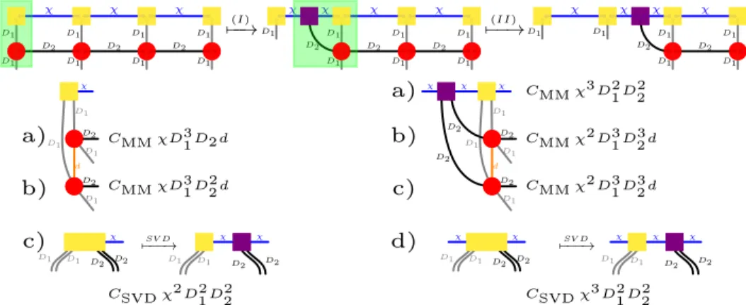
Before discussing contractions of tensor networks with varying bond dimension in the sub-sequent subsection, let us briefly comment on the computational complexity of exactly con-tracting the RVB state on the kagome lattice in regards to bond and border bond PEPS representations. One strategy employed to contract a PEPS on a lattice is to treat one boundary of the two PEPS layers as an MPS and to view the contraction of the remaining rows of PEPS tensors as the application of matrix product operators to this boundary MPS (see Figure 5 and 6). For a PEPS with bond dimension D on the kagome lattice the com-putational cost of the contraction of a single local tensor into the boundary MPS is given by
O(χ3D4) +O(χ2D6d) [45], withdthe physical dimension andχdenoting the bond dimension of the boundary MPS. However, since we do not reduce the bond dimension of the boundary MPSχ, we can omit the final SVD, and the relevant scaling is simply O(χ2D6d).
Contracting one full row of local PEPS tensors into the boundary MPS increases its bond dimension by a factor ofD2due to the double layer structure of the network, i.e. χi+1=D2χi.
In the case of an exact contraction, this bond dimension is not compressed after each step, and henceχgrows exponentially withD2. Accordingly, if we consider the computational cost of computing an expectation value of a PEPS with bond dimensionDon a 2(L+ 1)×2(L+ 1) lattice and taking into account that we can use a boundary MPS from both sides of the lattice,