Operator Limits of Random Matrices. Diane Holcomb

(1)

Operator Limits of Random Matrices

Diane Holcomb

with contributions from B´alint Vir´ag

These notes were written for a short course taught by myself, Diane Holcomb, at KTH in November-December of 2017. They incorporate notes written for a short course taught by Bálint Virág at PCMI summer school in July 2017 which were written as a collaboration between myself and Báling Virág. Portions of these notes will also be based on a random matrices course given by Benedek Valkó at University of Wisconsin circa Spring 2012.

The intention of the lectures here at KTH is to provide an introduction to the type of operator convergence work that is becoming better known in the random matrix community, but is still not widely studied or understood. Major contri-butions to this area include the work of Alan Edelman, Ioana Dumitriu, Brian Sutton, Jose Ram´ırez, Brian Rider, Bálint Virág, and Benedek Valkó. There will naturally be portions of the area that I will not be able to cover in full detail in the lecture. These notes will fill in some, though probably not all of these details. I also would like to make a few notes about the style and organization of the notes. The goal here is the introduction to the ideas underlying the field. Because of this I will not be doing things in full generality, nor proving common statements from random matrices. I hope that when I finish the notes each chapter will have a first section that gives in some sense the narrative of the chapter. The lectures will largely be drawn from these sections. Remaining sections will discuss the results from the chapter in greater generality and/or prove statements left unproven in the first section. The exception to this is chapter 1 which includes a variety of preliminaries that are necessary for the remainder of the notes. The current version is still very much a work in progress.

(2)

(3)

The Gaussian Ensembles

1. The Gaussian Orthogonal and Unitary Ensembles

One of the earliest random matrix models was introduced by Eugene Wigner in the 1950’s. The model can be characterized in many ways, but we will start with the following construction: let Mn be a symmetric matrix with

mij ∼ N(0,1) fori < j, and mii∼ N(0,2).

The symmetry condition completes the description of the matrix. A matrix con-structed in this way is said to be a member of the Gaussian Orthogonal Ensemble. If we instead take mij ∼ CN(0,1)∼ X+iY a complex standard normal where

X and Y are independent with N(0,1) distribution and the constraintMn=Mn∗

we get the Gaussian Unitary ensemble.

Theorem1.1. SupposeMn has GOE or GUE distribution thenMn has

eigen-value density (1) f(λ1, ..., λn) = 1 Zn n Y k=1 e−β4λ 2 k Y i<j |λi−λj|β

with β = 1 for the GOE and β = 2 for the GUE.

For convenience we will take Λ(n)={λi}ni=1 to denote the set of eigenvalues of

the GOE or GUE. This notation will be used later to denote the eigenvalues or points in whatever random matrix model is being discussed at the time.

Observe that for the joint density above we can move all the the terms into the exponent giving us that

f(λ1, ..., λn) = 1 Zn exp " −β 4 n X k=1 λ2_k+βX i<j log|λi −λj| # .

From this we can see that this is a model for n particles interacting through a Hamiltonian with a potential V(x) = x2 _{and an interaction term log}_|_x₋_y_|_.

These two terms work against each other, the potential term pushing the particles together while the interaction term pushes them apart. Now consider the what happens as n increases. The first sum has n terms while the second has n₂, therefore as n tends to infinity the repulsion will be the dominant term. This means that the points will be found further and further out and will not remain in a compact interval. To put these two terms on the same scale we do the mapping

(6)

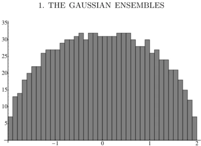
6 1. THE GAUSSIAN ENSEMBLES -1 0 1 2 5 10 15 20 25 30 35

Figure 1. Rescaled eigenvalues of a 1000×1000 GOE matrix λi 7→

√

nxi. Then the joint density for thexi’s will be given by

fx(x1, ..., xn) = e(n2)log √ n Znnn/2 exp " −nβ 4 n X k=1 x2_k+βX i<j log|xi−xj| # = e (n 2)log √ n Znnn/2 exp −n2β 4 Z x2dνn(x) +n2β Z Z log(x−y)dνn(x)dνn(y) , where here νn = _n1 Pn

k=1δxk is the empirical measure of the xi’s. Notice that the

original mapping was equivalent to scaling the eigenvalues down by a factor of√n

and so we get that

(2) νn= 1 n n X k=1 δ_λi/√ n.

If these measures converge asn → ∞it must be to the measure which minimizes the energy of the system with Hamiltonian

H∞(σ) = 1 2 Z x2dσ(x)− Z Z log(x−y)dσ(x)dσ(y).

This Hamiltonian is minimized by the semicircle measure σsc with density

dσsc dx = 1 2π √ 4−x2 ₁ x∈[−2,2] =ρsc(x).

Exercise 1.2. Show that σsc minimizes H∞.

Theorem 1.3 (Wigner’s semi-circle law). Let νn be the sequence of measures

defined in (2). Then as n→ ∞

νn ⇒σsc.

One way of thinking of this statement is to consider the histogram of the rescaled eigenvalues of a large GOE matrix. This histogram will be approximately semi-circular in shape. See figure 1. For a proof of the semicircle law involving graph convergence see chapter 2.

(7)

2. GLOBAL AND LOCAL CONVERGENCE 7

1.1. Properties of the GOE. One of the most important properties of the GOE after the fact that its eigenvalue density has an explicit form is that the distribution of the GOE is invariant under orthogonal conjugation.

Theorem 1.4. Let Mn have GOE distribution and O be an independent

or-thogonal matrix. Then Mn d

=OMnOt.

Before proving the above theorem we need to introduce at least one other description of the GOE.

Proposition1.5. The following characterizations of the Gaussian Orthogonal

Ensemble are equivalent:

(1) Mn=Mnt withmii ∼ N(0,2)andmij ∼ N(0,1)fori < jall independent.

(2) Mn= Xn+X t n

√

2 whre xi,j ∼ N(0,1) all independent.

(3) Mn has density _Z1 exp(−1₄Tr M MT) on the space of symmetric matrices.

Proof. If v is a standard normal vector and O is orthogonal then Ov =d v.

Therefore, for X = [v1, v2, ..., vn] i.i.d vectors we get OX d

= X. Then using the second description of the GOE we get that OXnOT

d

=Xn.

Alternatively, consider the third description of the GOE. We look at the trans-formation X 7→ OXOT_. _{The density will be invariant if we can show that}

Tr XXT _{= Tr} _OXOT₍_OXOT₎T _{and the Jacobian has a magnitude of 1.}

In-deed we do get the equality of the traces because conjugation with an orthogonal matrix fixes the eigenvalues. For the second part we need the following lemma:

Lemma 1.6. The Jacobian of X 7→OXOT is 1.

This completes the proof of the previous lemma

proof of lemma 1.6. Let vX = (x11, x22, ..., xnn, x12, x13, ..., xn−1,n)T. Then

there is a matrixAwithv_OT_XO =Av_X. We need|detA|. LetD=diag(1,1, ...,1,2, ...,2)

(n 1’s and (n2₋_n₎_/_{2 2’s). Then}

v_XTDvX = TrXXT

moreover we get that

v_XTATDAvX =vOT_XODv_OT_XO = TrXXT

Therefore ATDA = Dand so |detA|2_det_D _{= det}_D _{which implies} _|_det_A_| ₌

1.

Remark 1.7. Similar results hold for the GUE, but the orthogonal matrix O

is replaced by a unitary matrix U.

2. Global and local convergence

The Wigner semi-circle law is an example of a global or macroscopic conver-gence result. In this setting the rescaled eigenvalues{λi/

√ n}n

i=1 accumulate on a

compact interval and so in the limit become indistinguishable from each other. If we are instead interested in the local interactions between eigenvalues (the inter-actions of eigenvalues with their neighbors) we need to be able to see the behavior of individual points in the limit.

(8)

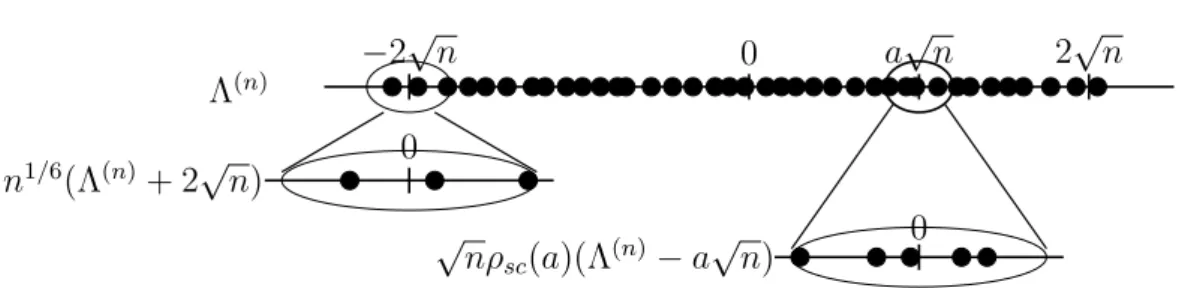
8 1. THE GAUSSIAN ENSEMBLES -2 0 2 Λ(n) √ n O(n−1₎ O(n−2/3₎ −2√n 0 2√n Λ(n) O(n−1/2₎ O(n−1/6₎

Figure 2. Spectrum of a GOE scaled down to [−2,2] and in natural scale.

Figure 2 shows the spectrum of a GOE on two different scales along with the order of magnitude of the spacing. Notice that at this point if we took n → ∞

for either Λ(n)/√n or Λ(n) all of the points would become indistinguishable even at the edge. To see where the spacing comes from consider the Wigner semi-circle law. When n is large we get that for a < b∈[−2,2]

#{xi =λi/ √ n ∈[a, b]} ≈n Z b a dσsc(x) = n Z b a 1 2π √ 4−x2_dx

When [a, b] = [a, a+δ] witha∈(−2,2−δ) this become approximately the length of the interval multiplied by ρsc evaluated at a. Therefore #{xi ∈[a, b]} ≈nδρsc(a)

(recall xi = λi/ √

n), meaning that there are order n points in any such interval and the approximate spacing of the points is O(1/n).

Exercise 2.1. Check that the number of points xi in an interval of the form

[−2,−2 +δ] is on the order of n2/3 _{meaning that the spacing is} _O₍_n−2/3_).

At this point we can see that the scale at which the points of a GOE will be order 1 about will change depending on the location. We call the set (−2√n,2√n) the bulk of the spectrum and the points ±2√n the edge. In the bulk of the spectrum we need to scale up byf(a)√n wheref(a) is some function ofa. At the edge we need to scale up by n1/6_{. See Figure 2 for a picture of what is happening.}

The limiting spectral measure (in this case the semi-circle) should be taken as a guide for the correct scale at which to see local interaction but is not guaranteed to give the right answer. In this case it does and we get the following results:

Theorem 2.2 ([7]). Let λ1 ≥ λ2 ≥ · · · denote the ordered eigenvalues of the

GOE then

n1/6(2√n−λi) _i₌₁_,...,k ⇒ {Λ1,Λ2, ...,Λk}

where Λi are the ordered eigenvalues of a certain random differential operator.

The differential operator and the theorem will be discussed in further detail in chapter 4.

Theorem 2.3 ([9],[10]). Let Λ(n) be the set of eigenvalues of a GOE and a∈(−2,2)then

ρsc(a) √

n(Λ(n)−a√n)⇒Sine1

where Sine1 is a point process that may be characterized as the eigenvalues of a

(9)

3. TRIDIAGONALIZATION AND SPECTRAL MEASURE 9 −2√n 0 2√n Λ(n) a√n n1/6_(Λ(n)_{+ 2}√_n₎ 0 √ nρsc(a)(Λ(n)−a √ n) 0

Figure 3. Illustration of the correct scale to see local interactions.

Remark 2.4. These theorems were originally proved and stated using the

in-tegrable structure of the GOE. The GOE eigenvalues form a Pfaffian point process with a kernel constructed from Hermite polynomials. The limiting processes may be identified to looking at the limit of the kernel in the appropriate scale.

3. Tridiagonalization and spectral measure

Up to this point we have discussing the empirical measure associated to the eigenvalues, but there is another measure that we can discuss which will turn out to be useful. That is the spectral measure of a matrix A at a vector v. For this section we will always take v =e1 the first coordinate vector.

Definition 3.1. Suppose you have a symmetric matrix A, we can define its

spectral measure (at the first coordinate vector) σA. The spectral measure is the

measure for which

Z

xkdσA=Ak11.

Exercise 3.2. Check that if λ1, ..., λn are the eigenvalues of A then

σA=

X

i

δλiϕi(1)2

where ϕi is the ith normalized eigenvector ofA.

We say two symmetric matrices are equivalent if they have the same eigen-values with multiplicity. This equivalence is well understood: two matrices are equivalent if and only if they are conjugates by an orthogonal matrix (in group theory language, the equivalence classes are the orbits of the conjugation action of the orthogonal group). There is a canonical representative in each class, a diagonal matrix with non-increasing diagonals.

Can we have a similar characterization for matrices with the same same spec-tral measure?

Definition 3.3. A vectorv is cyclic for an n×n matrixA if v, Av, ..., An−1v

is a basis for the vector space _Rn.

Theorem 3.4. Let A and B be two matrices, then σA = σB if an only if

O−1_AO₌_B _where _O _{is orthogonal of the form} _O

11= 1, O1i = 0 for i6= 1.

Definition 3.5. A Jacobi matrix is a real symmetric tridiagonal matrix with

(10)

10 1. THE GAUSSIAN ENSEMBLES

Theorem 3.6. For allA there exists a unique Jacobi matrix J such thatσJ =

σA

Proof of Existence. We will use the Householder transformation to take

ann×n symmetric matrix to a similar tridiagonal matrix. Write our matrix in a block form, A= a bt b C

Now let O be an (n−1)×(n−1) orthogonal matrix, and let

Q=

1 0 0 O

Then Q is orthogonal and

QAQt=

a (Ob)t

Ob OCOt

Now we can choose the orthogonal matrixO so that Ouis in the direction of the first coordinate vector, namely Ou=|u|e1.

An expliction option for O is the following Householder reflection:

Ov =v−2hv, wi hw, wiw where w=b− |b|e1 Check that OOt=I,Ob =|b|e1. Therefore QAQt=       a |b| 0 . . . 0 |b| 0 .. . OCOt 0       .

We now repeat the previous step, but this time choosing the first two rows and columns to be 0 except having 1’s in the diagonal entries, and than again until

the matrix becomes tridiagonal.

Exercise 3.7. Suppose e1 is cyclic. Apply Gram-Schmidt to the vectors

(e1, Ae1, ..., An−1) to get a new orthonormal basis. Show that A written in this

basis will be a Jacobi matrix.

Exercise 3.8. A tridiagonal matrix J is called a Jacobi matrix if the off

diagonal entries are all positive. We define the spectrum of J to be the measure that satisfies R p(x)dσ(x) = he1, p(A)e1i for all polynomials p(x). Show that if J

and J0 are two Jacobi matrices withσJ =σJ0 then J =J0.

Hint: Look at the moments of the measure.

3.1. Tridiagonalization and the GOE. When we do this tridiagonalization procedure to the GOE we get a very clean result because of the invariance of the distribution under independent orthogonal transformation.

(11)

4. β-ENSEMBLES 11 Proposition 3.9 ([8]). Let A be GOEn. There exists a random orthogonal

matrix fixing the first coordinate vector e so that

OAOt=         a1 b1 0 . . . 0 b1 a2 . .. 0 . .. ... ... .. . . .. an−1 bn−1 0 bn−1 an        

with all entries indepdent,ai ∼ N(0,2)and bi ∼χn−i. In particular,OAOt =has

the same spectral measure as A.

For those unfamiliar with the chi distribution we make the following obser-vations. Suppose that k is an integer and v is a vector of independent N(0,1) random variables of lengthk, thenχk

d

=kvk. The density of aχrandom for k >0 is given by

fχk(x) =

1 2k2−1Γ(k/2)

xk−1e−x2/2,

where Γ(x) is the Gamma function.

Proof. The argument above can be applied to the random matrix. After the

first step, OCOt will be independent of a, band have a GOE distribution. This is because GOE is invariant by conjugation with a fixed O, andO is only a function of b. So conditionally on a,b, both C and OCOt _{have GOE distribution.}

Exercise 3.10. Let Xn×m be an n×m matrix with xi,j ∼ N(0,1) (not

sym-metric nor Hermitian). The distribution of this matrix is invariant under left and right multiplication by independent Unitary matrices. Show that such a matrixX

may be lower bidiagonalized such that the distribution of the singular values is the same for both matrices. Note that the singular values of a matrix are unchanged by multiplication by a unitary matrix.

(1) Start by coming up with a matrix that right multiplied withA gives you a matrix where the first row is 0 except the 11 entry.

(2) What can you say about the distribution of the rest of the matrix after this transformation to the first row?

(3) Next apply a left multiplication. Continue using right and left multipli-cation to finish the bidiagonalization.

4. β-ensembles

Exercise 4.1. For every spectral measure σ there exists a symmetric matrix

with that spectral measure. This implies that there exists a Jacobi matrix with this spectral measure.

(12)

12 1. THE GAUSSIAN ENSEMBLES Let An= 1 √ β         a1 b1 0 . . . 0 b1 a2 . .. 0 . .. ... ... .. . . .. an−1 bn−1 0 bn−1 an        

That is a tridiagonal matrix with a1, a2, ..., an ∼ N(0,2) on the diagonal and

b1, ..., bn−1 with bk ∼χβ(n−k) and everything independent. Recall that if z1, z2, ...

are iid N(0,1) thenz2₁ +· · ·+z_k2 ∼χ2_k.

Ifβ = 1 thenAnis similar to a GOE matrix (the joint density of the eigenvalues

is the same). If β = 2 then An is similar to a GUE matrix.

Theorem 4.2 ([2]). If β >0 then the joint density of the eigenvalue of An is

given by f(λ1, ..., λn) = 1 Zn,β e−β4 Pn i=1λ2i Y 1≤i<j≤n |λi−λj|β.

Before we start the proof we begin with a few observations. In the matrixAn

the off-diagonal entries are bi >0, and there are 2n−1 variable in the matrix.

We wish to compute the Jacobian of the map (λ, q) → (a, b). To do this we work by going through the moments.

mk =

Z

xkdσ =Xλk_iq_i2

We look at maps from both sets to (m1, ..., m2n−1). These are simple

transforma-tions. We will write down the appropriate matrices and hope we can find their determinants. F

Theorem 4.3 (Dumitriu, Edelman, Krishnapur, Rider, Vir´ag, [2, 5]). Let V

be a potential (think convex) and a, bare chosen from then density proportional to

exp (−TrV(J))

n−1

Y

k=1

bkβ_n₋−_k1

then the eigenvalues have distribution

f(λ1, .., λn) = 1 Z exp − X i V(λi) ! Y i<j |λi−λj|β

and the qi are independent of the λ with (q1, ..., qn) = (ϕ1(1)2, ..., ϕn(1)2) have

dirichlet(β₂, ...,β₂) distribution.

Suppose we have the sequence {(ai, bi), i ≥ 1} with the distribution from the

theorem. This is a Markov Chain. This holds no matter which polynomial you choose, though you might need to take bigger blocks of (ai, bi).

(13)

4. β-ENSEMBLES 13

4.1. Theβ-Laguerre ensemble. We finish this section by introducing a few more classical random matrix models and their associated β-ensembles. Suppose that you have a rectangular matrixn×pmatrix Xn withp≥n andxi,j ∼ N(0,1)

all independent. The matrix

Mn=XnXnt

is a symmetric matrix which may be thought of as a sample covariance matrix for a population with independent normally distributed traits. As in the case of the Gaussian ensembles we could have started with complex entries and looked instead at XX∗ to form a Hermitian matrix. The eigenvalues of this matrix have distribution (3) fL,β(λ1, ..., λn) = 1 Zβ,n,p n Y i=1 λ β 2(p−n+1)−1 i e −β 2λi Y j<k |λj −λk|β,

with β = 1. This generalizes to the β-Laguerre ensemble which is a set of points with densityfL,β. The matrix model Mnis part of a wider class of random matrix

models called Wishart matrices. This class of models was originally introduced by Eugene Wigner in the 1920’s.

As in the case of the Gaussian ensembles there is a limiting spectral measure when the eigenvalues are in the correct scale.

Theorem 4.4 (Marchenko-Pastur law). Let λ1, ..., λn have β-Laguerre

distri-bution, νn= 1 n n X i=1 δλi/n,

and suppose that n_p →γ ∈(0,1]. Then as n→ ∞

(4) νn ⇒σmp, where dσmp dx =ρmp(x) = p (γ+−x)(x−γ−) 2πγx 1[γ−,γ+], and γ± = (1± √ γ)2.

Notice that this density can display different behavior at the lower end point depending on the value of γ. In particular if γ = 1 then γ− = 0 and so the lower end of the spectrum is 0 and the density simplifies to.

ρmp(x) = 1 2π r 4−x x 1[0,4].

In this case the lower edge has an asymptote at 0, however for any γ <1 we get that the lower edge has the same √xtype behavior that we see at the edge of the semi-circle distribution.

As in the case of the β-Hermite ensemble there exists a tridiagonal matrix model which has joint eigenvalue distribution fL,β.

Theorem 4.5. Let Lβ,p= 1 √ β       χβp χ˜β(n−1) χβ(p−1) χ˜β(n−2) . .. . .. χβ(p−n+2) χ˜β χβ(p−n+1)      

(14)

14 1. THE GAUSSIAN ENSEMBLES

with the χ and χ˜ random variables independent χ-distributed random variables with the parameter given by the subscript. Then the eigenvalues of Lβ,pLtβ,p have

β-Laguerre distribution give in equation (3).

4.2. Circularβ-ensemble. We introduce one final classicalβ-ensemble. The circular orthogonal and unitary ensembles are defined by choosing an orthogonal or unitary matrix according to Haar measure on the spaces of orthogonal or unitary matrices respectively. When a matrix is chosen according to this distribution its eigenvalues fall on the circle and their joint density is given by

(5) fC(eiθ1, ..., eiθn) = 1 Z Y j<k |eiθj−eiθk|β

with β = 1 or 2 for the orthogonal or unitary ensembles respectively. A set of points on the circle that has joint density (5) is call a circular β-ensemble. This matrix model does not have a corresponding tridiagonal representation. Instead there is a corresponding matrix model called a CMV matrix which is a 5-diagonal matrix with a particular structure. This CMV matrix may be defined by looking at a sequence of numbers called Verblunsky coefficients. These coefficients will be discussed further in Chapter 6.

(15)

CHAPTER 2

The Wigner semi-circle law

1. Graph convergence

The proof of the Wigner semi-circle law given here will rest on a graph conver-gence argument, so we begin by introducing the notions of converconver-gence needed for the proof and the connection between graph and spectral convergence. We will try to give examples throughout this section so the precise nature of the convergence is easier to understand.

Example 1.1. Suppose thatA is the adjacency matrix of a graphG. We can

label the vertex corresponding to the first coordinate vector. ThenAk

11 is the sum

over weighted paths that are length k and return to the starting vertex.

What is the connection between graph convergence and spectral measure? We will be interested in taking limits of rooted graphs. The notion of spectral measure will be useful in this context. In particular we can define the spectral measure of a rooted graph in the following way:

Definition 1.2. Let (G, ρ) be a rooted graph and AG its adjacency matrix

whereρcorresponds to the first coordinate vector. We define the spectral measure of G rooted atρ to be the spectral measure of AG.

Definition 1.3. Suppose you have a sequence of graphs Gn with a

distin-guished vertex we call the root. We say that a sequence of graphs converges if any ball around the root stabilizes at some point.

Examples 1.4. We give two examples

(1) Suppose we take the n cycle with any vertex chosen as the root. This converges to _Zin the limit

(2) Suppose we have the k by k grid with vertices at the intersection. If we choose a vertex at the center of the grid as the root, we will get convergence to_Z2_.

Proposition 1.5. If (Gn, ρn) converges to (G, ρ) is the sense of rooted local

convergence, then the spectral measure of the graphs converge.

Exercise 1.6. Consider paths of length n rooted at the left end point. This

sequence converges to_Z+in the limit. What is the limit of the spectrum? It is the

· · · → · · · ·

Figure 1. Rooted n-cycles toZ

(16)

16 2. THE WIGNER SEMI-CIRCLE LAW

Wigner semi-circle law, since the moments are Dyck paths. But one can prove this directly, since the paths on length n are easy to diagonalize. This is an example where the spectral measure has a different limit than the eigenvalue distribution.

Definition 1.7. Suppose you wish to construct a graph on n vertices with a

given degree sequence (d1, ..., dn). The configuration model may be constructed

by attaching the appropriate number of half edges to the vertices and choosing a uniformly at random perfect matching of the half edges.

Exercise 1.8. Suppose you have the random d-regular graph onn vertices in

the configuration model. Then in the limit this converges to thed-regular infinite tree in the limit.

Definition 1.9. Benjamini-Schramm convergence: We define this

conver-gence for unrooted graphs. Choose a vertex uniformly at random to be the root. If this converges in distribution in with respect to rooted convergence to a random rooted graph, we say the graphs converge in this sense.

This is essentially asking for convergence of the local statistics.

Proposition 1.10. Suppose we have a finite graph G and we choose a vertex

uniformly at random. This defines a random graph and its associated random spectral measure σ. Then Eσ =µis the eigenvalue distribution.

Proof. Recall that for the spectral measure of a matrix (and so a graph) we

have σ(G,ρ)= n X i=1 δλiϕ2i(ρ)

Since ϕi is of length one, we have

X ρ∈V(G) ϕi(ρ)2 = 1 hence EσG,ρ= 1 n X ρ∈V(G) σG,ρ =µG.

Examples 1.11. The following are examples of Banjamini-Schram

conver-gence:

(1) A cycle graph converges to the graph of _Z. (2) A path of lengthn converges to the graph of _Z. (3) Large box ofZd converges to the full Zd lattice.

Notice that for the last two the probability of being in a neighborhood of the edge goes to 0 and so the limiting graph doesn’t see the edge effects.

Exercise 1.12. Say a sequence of d-regular graphs Gn with n vertices is of

essentially large girth if for every k the number of k-cycles in Gn is o(n). Show

that Gn is essentially large girth if and only if it Benjamini-Schramm converges

(17)

1. GRAPH CONVERGENCE 17 Exercise 1.13. (harder) Show that for d ≥ 3 the d-regular tree is not the

Benjamini-Schramm limit of finite trees.

How does this help? We will get that σn → σ∞ in distribution and also in expectation. By bounded convergence, the eigenvalue distributions will converge as well: µn=Eσn→Eσ∞.

We can also consider the case whereG are weighted graphs. This corresponds to general symmetric matrices A. In this case we require that the neighborhoods stabilize and the weights also converge. Everything goes through.

Example 1.14 (The spectral measure of Z). We use Bejamini-Schram

con-vergence of the cycle graph to _Z. We begin by computing the spectral measure of the n-cycle Gn. We get that A=T +Tt where

T =        0 1 0 1 . .. ... . .. 1 1 0       

The eigenvalues of 2T will be the roots of unity. We can think of this as A = (T+T₂−1)2. So think of this as having the eigenvalues uniformly spaced on a circle of radius 2. The spectrum will be given by the projection of these points onto the real line. In the limit this will become the projection of the uniform measure on the circle. This gives you the arcsine distribution.

σ_Z= 1

2π√4−x21x∈[−2,2]dx

Exercise 1.15. Let Bn be the unweighted finite binary tree with n levels.

Suppose a vertex is chosen uniformly at random from the set of vertices. Give the distribution of the limiting graph.

Exercise 1.16. Let (G, ρ) be a rooted graph, we define the spectrum of

(G, ρ) to be the measure that satisfies that for all polynomials p(x) we get that

R

p(x)dµ(x) = he1, p(A)e1i where we take the root to correspond to the first row

and column of the matrix.

(1) Suppose a graph Gn has the n×n adjacency matrix

A=        0 1 1 0 1 1 . .. ... . .. 0 1 1 0       

What is the graph with adjacency matrix A?

(2) Suppose we root Gn at the vertex corresponding to the first row and

column. What is limit of (Gn, ρn)?

(3) Suppose we choose the root uniformly at random. What is the limit of the graph? What is the spectrum of the limiting graph? This is a distribution you have seen before.

(18)

18 2. THE WIGNER SEMI-CIRCLE LAW

Exercise 1.17. Let A be a rescaled n × n Dumitriu-Edelman tridiagonal

matrix A= √1 βn        b1 a1 a1 b2 a2 a2 . .. ... . .. bn−1 an−1 an−1 bn        , ai ∼χβ(n−i), bi ∼ N(0,1)

all independent, and suppose that Ais the adjacency matrix of a weighted graph. (1) Draw the graph with adjacency matrix A. (There can be loops)

(2) Suppose a root for your graph is chosen uniformly at random, what is the limiting distribution of your graph?

(3) What is the limiting spectral measure of the graph rooted at the vertex corresponding to the first row and column?

(4) What is the limiting spectral measure of the unweighted graph?

2. Wigner semicircle law

Note that a Jacobi matrix can be thought of the adjacency matrix of a weighted path with loops.

Exercise 2.1. Check that χn− √

n −−−→P

n→∞ N(0,1/2).

Proof 1. Take the previous graph, divide all the labels by √nand then take

a Benjamini-Schramm limit.

What is the limit? _Z, but then we need labels. The labels in a randomly rooted neighborhood will now be the square root of a single uniform random variable in [0,1]. Call thisU. Then the edge weights are √U. Recall thatµn →Eσ. In the

case where U was fixed we would just get a scaled arcsine measure.

Choose a point uniformly on the circle of radius √U and project it down to the real line. But this point is in fact a uniform random point in the disk. This gives us the semicircle law.

µsc = 1 2π √ 4−x2₁ x∈[−2,2]dx. Proof 2. We take the rooted limit where we choose the root to be the matrix J/√n corresponding to the first coordinate vector.

In the limit this graph converges to _Z+. Therefore σn → σZ+ = ρsc. This

convergence is weak convergence in probability.

So going back to the full matrix model of GOE, we see that the spectral measure at an arbitrary root converges weakly in probability toµsc. But then this

must hold also if we average the spectral measures over the choice of root (but not the randomness in the matrix).

Thus we getµn→µsc in probability.

Dilemma: The limit of the spectral measure should have nothing to do with the limit of the eigenvalue distribution in the general case. This tells you that the Jacobi matrices that we get in the case of the GOE are very special.

(19)

CHAPTER 3

The top eigenvalue and the Baik-Ben Arous-Pechet

transition

1. The top eigenvalue

The eigenvalue distribution of the GOE converges after scaling by √n to the Wigner semi-circle law. From this, it follows that the top eigenvalue,λ1(n) satisfies

for every ε >0

P(λ1(n)/

√

n >2−ε)→1

the 2 here is the top of the support of the semicircle law. However, the upper bound does not follow and needs more work. This is the content of the following theorem.

Theorem 1.1 (F¨uredi-Koml´os). λ1(n)

√

n →2 in probability.

This holds for more general Wigner matrices; we have a simple proof for the GOE case.

Lemma 1.2. If J is a Jacobi matrix (a’s diagonal, b’s off-diagonal) then λ1(J)≤max

i (ai+bi+bi−1)

Here we take the convention b0 =bn = 0.

Proof. Observe that J may be written as

J =−AAT + diag(ai+bi+bi−1) where A=      0 √b1 −√b1 √ b2 −√b2 √ b3 . .. ...     

and AAt _{is nonnegative definite. So for the top eigenvalues we have}

λ1(J)≤ −λ1(AAT) +λ1(diag(ai+bi+bi−1))≤max

i (ai +bi+bi−1).

We used sublinearity of λ1, which follows from the Rayleigh quotient

representa-tion.

If we apply this to our setting we get that

λ1(GOE)≤max

i (Ni, χn−i+χn−i+1)≤2 √

n+cplogn

(20)

20 3. THE TOP EIGENVALUE AND THE BAIK-BEN AROUS-PECHET TRANSITION

the right inequality is an exercise (using the Gaussian tails in χ) and holds with probability tending to 1 ifcis large enough. This completes the proof of Theorem 1.1.

This gives you that the top eigenvalue cannot go further than an extra logn

outside of the spectrum. Indeed we have that

λ1(GOE) = 2

√

n+T W1n−1/6+o(n−1/6)

so this result from before is not optimal.

2. Baik-Ben Arous-Pechet transition

Historically one of the areas that random matrices have been used is to study correlations. When considering principle component analysis we use the Wishart model to study what would happen if we just had noise and nothing else? How likely is it that the correlations that we see are more than chance?

Wishart consider matrices Xn×m with independent entries and studies the

eigenvalues ofXXt. We will take the noise matrixX to have i.i.d. normal entries. We study rank one perturbations and consider the top eigenvalue. Consider the case n =m. Theorem 2.1 (BBP transition). 1 nλ1 Xdiag(1 +a2,1,1, ...,1)Xt→ϕ(a)2 where ϕ(a) = ( 2 a ≤1 a+ 1_a a ≥1

Heuristically, correlation in the populations appears in the asymptotics in the top eigenvalue of the data only if it is sufficiently large, a >1. Otherwise, it gets washed out by the fake correlations coming from noise.

We will prove the GOE analouge of this theorem, and leave the Wishart case as an exercise.

One can also study the fluctuations of the eigenvalues. In the case a < 1 you get Tracy-Widom. In the case a >1 you get Gaussian fluctuations. Very close to th point a= 1 you get a deformed Tracy-Widom.

The GOE analogue is the following.

Theorem 2.2 (Top eigenvalue of GOE with nontrivial mean). λ1(GOEn+

a √

n11

t₎_→_ϕ₍_a₎

where 1 is the all-1 vector, and 11t _{is the all-1 matrix.}

It may be suprising how little change in the mean in fact changes the top eigenvalue!

We will not use the following theorem, but will include it only to show where the function φ comes from. It will also motivate the proof for the GOE case.

Theorem 2.3.

(21)

2. BAIK-BEN AROUS-PECHET TRANSITION 21

We will leave this as an exercise for the reader.

Heuristics. The spectrum of Z+ is absolutely continuous. This doesn’t change unless a is big enough. Why? there is an eigenvector (1, a−1_{, a}−2_{, ...}₎

which is only in `2 _when _{a >}_{1. Moreover this has eigenvalue} _a₊ 1

a.

Proof of GOE case. The first observation is that because the GOE is an

invariant ensemble, we can replace 11t _by _vvt _{for any vector} _v _{having the same}

length as the vector 1. We can replace the perturbation with √nae1et1. Such

perturbations commute with tridiagonalization.

Therefore we can consider Jacobi matrices of the form

J(a) = √1 n   a√n+N1 χn−1 χn−1 N2 χn−2 . .. . .. ...  

Case 1: a ≤1. Since the perturbation is positive, we only need an upper bound. We use the maximum bound from before. For i = 1, the first entry, there was a room of size √n. For i= 1 the max bound still holds.

Case 2: a >1

Now fix k and let v = (1,1/a,1/a2_{, ...,}₁_/ak_,₀_{, ...,}_{0). We get that the error}

from the noise will be of order 1/√n so that

J(a) v −v(a+ 1 a) ≤ca−k

with probability tending to 1.

Now if for a symmetric matrix A and a vector v of length at least 1 we have

kAv−xvk< ε, then A has an eigenvalueε-close tox.

ThusJ(a) has an eigenvalue λ∗ that is ca−k-close to a+ 1/a.

We now need to check that this eigenvalue will actually be the maximum.

Lemma 2.4. Consider adding a positive rank 1 perturbation to a symmetric

matrix. Then the eigenvalues of the two matrices will interlace and the shift under perturbation will be to the right.

By interlacing,

λ2(J(a))≤λ1(J) = 2 +o(1) < a+ 1/a−cak

if we chosek large enough. Thus the eigenvalue λ∗ we identified must be λ1.

Exercise2.5. Suppose you haveZ+with a loop of weightaon the end and let

λ1(a) be the largest eigenvalue the graph. We can think of this as a rank 1 positive

definite pertubation of _Z+_{. By interlacing this means that the largest eigenvalue}

will shift to the right under the perturbation. Prove the following lower bound:

(6) λ1(a)≥

(

2 a≤1

(22)

(23)

CHAPTER 4

The soft edge

1. The heuristic convergence argument

The distribution of top eigenvalue of the β-Hermite ensemble has nice closed formulas in the case ofβ = 1,2,4. The goal here is to give the characterization of the top eigenvalue for general β. To do this we look at the geometric structure of the tridiagonal matrix.

Simulations show that the eigenvectors corresponding to the top eigenvalues of the matrix tend to be supported in the first o(n) coordinates. This suggests that we in some sense need to look at the top corner of the matrix in order to see the behavior of the top eigenvalue.

Now suppose that you have the matrix

A=      0 1 1 0 1 1 0 . .. . .. ...     

We look at the matrix A−2I, and we look at the action of this matrix on the first order m entries of a vector, where we guess that m = nα, with α to be determined later. Let f :_R+ → _R and vf = (f(0), f(1/m), f(2/m), ..., f(n/m))t.

Then B =m2₍_A₋₂_I_{) acts as a discrete second derivative on}_f_{, in the sense that}

Bvf ≈vf00.

Returning to the β-Hermite case, by Exercise 2.1, for k n we have

χn−k ≈

p

β(n−k) +N(0,1/2)≈pβ(√n− k

2√n) +N(0,1/2)

Now we consider the matrix

mγ(2√nI −J)≈ mγ√n      2 −1 −1 2 −1 −1 0 . .. . .. ...      + m γ 2√n        0 1 1 0 2 2 0 3 3 0 . .. . .. ...        + m γ √ β      N1 N˜1 ˜ N1 N2 N˜2 ˜ N2 N3 . .. . .. ...      23

(24)

24 4. THE SOFT EDGE

Now assume that we havem=nα _{for some} _α_{. What choice of}_α_{should we make?}

For the first term we want

mγ√n      2 −1 −1 2 −1 −1 0 . .. . .. ...     

to behave like a second derivative. This means that mγ√n = m2 which gives 2α = αγ + 1/2. We do a similar analysis on the second term. We want this term to behave like multiplication by t. for this we want m√γ

n =

1

m which gives

αγ −1/2 = −α. Solving this system we get α = 1/3 and γ = 1/2. For the noise term, multiplication by it should yield a distribution (in the Schwarz sense), which means that its integral over intervals should be of order 1. In other words, the average of m noise terms times mγ should be of order 1. This gives γ = 1/2, consistent with the previous computations.

This means that we need to look at the section of the matrix that is m=n1/3

and we rescale by n1/6_{. That is we look at the matrix}

n1/6(2√n−Jn)

acting on functions with mesh size n−1/3_.

Exercise 1.1. Show that in this scaling, the second matrix in the expansion

above has the same limit as the diagonal matrix with 0,2,4,5,6, ....on the diagonal (scaled the same way).

The final piece that we need to check is what happens to the final matrix with noise terms. We may use a similar trick to the previous exercise in order to consider the matrix given by

Wn =      N1 N2+ 2 ˜N1 N3+ 2 ˜N2 . ..     

With the exception of the first entry all the of the diagonal entries are now inde-pendent 2N(0,1). In order to consider the action of Wn on a vector vf we need

to look at the ‘integrated version’ via Riemann sums. In particular we consider

m1/2 √ β bxmc X k=1 1 m(Wnvf)k = m−1/2 √ β bxmc X k=1 Wkkf(k/m).

(25)

1. THE HEURISTIC CONVERGENCE ARGUMENT 25

and we consider the entries ofWnto be the increments of some process Y(x) with

Y(k

m)−Y( k−1

m ) = m−1/2

2 Wkk. Then we may write

m−1/2 √ β bxmc X k=1 (Wnvf)k = 2 √ β bxmc X k=1 f(_mk) Y(_mk)−Y(k_m−1) ≈ √2 β bxmc X k=1 f(_mk)−f(k_m−1) Y(_mk) ≈ √2 β 1 m bxmc X k=1 f0(_mk)Y(_mk)⇒ √2 β Z x 0 f0(s)bsds

We’ve integrated and done an integration by parts here, so the noise term should actually give a contribution of √2

βb

0

x in the limit.

Conclusion. This matrix acting on functions with this mesh size behaves like a differential operator. That is

Hn =n1/6(2 √ n−Jn)≈ −∂x2+x+ 2 √ βb 0 x = SAOβ

here b0_x is a white noise. This operator will be called the Stochastic Airy operator (SAOβ). We also set the boundary condition to be Dirichlet. This conclusion can

be made precise.

There are two problems at this point that must be overcome in order to make this convergence rigorous. The first is that we need to actually be able to make sense of that limiting operator. The second is that the matrix even embedded an an operator on step functions acts on a different space that the SAOβ so we

need to make sense of what the convergence statement should actually be. The following are the main ideas behind the operator convergence.

Ideas on the operator convergence. (1) Embed_Rn intoL2(_R) via

ei 7→ √ m1_[i−1 m , i m).

This gives an embedding of the matrixJ acting on a subspace of L2(_R+). (2) It is not clear what functions the Stochastic Airy Operator acts on at this point. Certainly nice functions multiplied by the derivative of Brownian motion will not be functions, but distributions. The only way we get nice functions as results if this is cancelled out by the second derivative. Nevertheless, the domain of SAOβ can be defined.

In any case, these operators act on two completely different sets of functions. The matrix acts on piecewise constant functions, while SAOβ

acts on some exotic functions.

(3) The nice thing is that if there are no zero eigenvalues, bothH−1

n and J

−1

can be defined in their own domains, and the resulting operators have compact extensions to the entireL2_.

The sense of convergence we have is

(26)

26 4. THE SOFT EDGE

This is called norm resolvent convergence, and it implies convergence of eigenvalues and eigenvectors if the limit has discrete simple spectrum. (4) The simplest way to deal with the limiting operator and the issues of

white noise is to think of it as a bilinear form. This is the approach we follow in the next section. Thekth eigenvalue can be identified using the Courant-Fisher characterization.

Exercise1.2. We will consider cases where a matrixAn×ncan be embedded as

an operator acting on the space of step function with mesh size 1/mn. In particular

we can encode these step functions in to vectorsvf = [f(_mn1 ), f(_mn2 ), ..., f(_mnn )]t.

LetA be the matrix

A=     −1 1 −1 1 . .. ... −1    

For which kn to we get knAvf →f0?

Exercise 1.3. LetAbe the diagonal matrix with diagonal entries (1,4..., n2).

Find a kn such that knAvf converges to something nontrivial in the limit. What

is kn and what does the limit converge to?

Exercise1.4. LetJ be a Jacobi matrix (tridiagonal with positive off-diagonal

entries) and v be an eigenvector with eigenvalue λ. The number of times that v

changes sign is equal to the number of eigenvalues above λ. More generally the equation J v = λv determines a recurrence for the entries of v. If we run this recurrence for an arbitraryλ(not necessarily an eigenvalue) and count the number of times thatv changes sign this still gives the number of eigenvalues greater than

λ.

(1) Based on this gives a description of the number of eigenvalues in the interval [a, b].

(2) Suppose that vt _{= (}_v

1, ..., vn) solves the recurrence defined by J v = λv.

What is the recurrence for rk =vk+1/vk? What are the boundary

condi-tions forr that would make v and eigenvector?

2. The bilinear form and making sense of the SAOβ

Recall the Airy operator

Af =−∂_x2+xf

acting on L2₍

R+) with boundary condition f(0) = 0. The equation Af = 0 has two solutions Ai(x) and Bi(x), called Airy functions. Note that the solution of (A−λ)f = 0 is just a shift of these functions byλ.

Since only Ai2 _{is integrable, the eigenfunctions}_A _{are the shifts of Ai with the}

eigenvalues the amount of the shift. We know that thekth zero of the Ai function is atzk =− 3₂πk

2/3

+o(1),therefore to satisfy the boundary conditions the shift must place a 0 at 0, so thekth eigenvalue is given by

(7) λk=−zk = 3 2πk 2/3 +o(1)

(27)

2. THE BILINEAR FORM AND MAKING SENSE OF THE SAOβ 27

The asymptotics are classical.

For the Airy operator A and a.e. differentiable, continuous functions f with

f(0) = 0 we can define

kfk2∗ :=hAf, fi=

Z ∞

0

f2(x)x+f0(x)2 dx.

LetL∗ be the space of such functions with kfk∗ <∞

Exercise 2.1. Show that there is c >0 so that kfk2 ≤ckfk∗ for every f ∈L∗. In particular,L∗ ⊂L2_.

Recall the Rayleigh quotient characterization of the eigenvalues λ1 of A.

λ1 = inf

f∈L∗_,_k_f_k 2=1

hAf, fi.

More generally, the Courant-Fisher characterization is

λk = inf

B⊂L∗_,_dim_B₌_k sup

f∈B,kfk2=1

hAf, fi

where the infimum is over subspaces B.

For two operators we sayA ≤B if any f ∈L∗ hf, Afi ≤ hf, Bfi. Exercise 2.2. If A≤B, then λk(A)≤λk(B).

Our next goal is to define the bilinear form associated with the Stochastic Airy operator on funcitons in L∗. Clearly, the only missing part is to define

Z ∞

0

f2(x)b0(x)dx.

At this point you could say that this is defined in terms of stochastic integration, but the standard L2 theory is not strong enough – we need it to be defined in the almost sure sense for all functions in L∗. We could define it in the following way:

hf, b0fi“ = ” Z ∞ 0 f2(x)b0(x)dx=− Z ∞ 0 2f0(x)f(x)b(x)dx

This is now a perfectly fine integral, but it may not converge. The main idea will be to write b as its average together with an extra term.

b(x) =

Z x+1

x

b(s)ds+ ˜b(x) = ¯b(x) + ˜b(x)

In this decomposition we will get that ¯b is differentiable and ˜b is small. The averaging term decouples quickly (at time intervals of length 1), so this term is analogous to a sequence of i.i.d. random variables. We define the inner product in terms of this decomposition

hf, b0fi:= Z ∞ 0 f2(x)¯b0(x)dx−2 Z ∞ 0 f0(x)f(x)˜b(x)dx.

(28)

28 4. THE SOFT EDGE

Exercise2.3. There exists a random constantC so that we have the following

inequality of functions:

(8) |¯b0|,|˜b| ≤Cplog(2 +x)

Now we return to the Stochastic Airy operator, the following lemma with give us that the operator is bounded from below.

Lemma 2.4. We have

−CI+ (1−ε)A≤SAOβ ≤(1 +ε)A+CI

for some random constant C. This may also be written as (9) −Ckfk2

2 + (1−ε)kfk2∗ ≤ hf,SAOβfi ≤(1 +ε)kfk2∗+Ckfk22

The upper bound here implies that the bilinear form is defined for all functions

f ∈L∗. The lemma will follow from the fact that

b0 ≤ε(1 +ε)A+cI,

in the sense of operators.

Proposition2.5. The eigenvalues of SAOβ admit a variational

characteriza-tion.

Proof for Λ0. Let ˜Λ0 = inf{hf,SAOβi : f ∈ L∗,kfk2 = 1}, then we may

choose a minimizing sequence fn ∈ L∗,kfnk2 = 1 with hfn,SAOβi → Λ˜0. From

equation (9) we get that thefnmay be chosen so thatkfnk∗ ≤Bfor some constant

B(a function of the brownian path). Therefore we can choose a subsequence which converges to some function f0 uniformly on compact subsets, in L2, and weakly

in H1_{. Using bounds on ˜}_b _{and ¯}_b _{from equation (8) we get that for} _{ε >} _{0 we may}

choose X so that hfn,SAOβfni=kfk2∗− kfk22+ 4 √ β Z X 0 f(x)f0(x)b0(x)dx+E where |E| ≤εkfk2

∗. Taking the limit as n → ∞ we see that the middle two terms converge and kf0k2∗ ≤ lim infkfnk2∗. Taking ε → 0 we get that hf0,SAOβfi ≤

˜

Λ0. The definition of ˜Λ0 gives the opposite inequality. Therefore we have that

hf0,SAOβfi = ˜Λ0 meaning that the infimum is achieved at some function f0. It

remains to be shown that f0 is an eigenfunction, that is, for any test function ϕ

we have hϕ,SAOβf0i= Λhϕ, f0i. Look at f = f0+ϕ kf0+ϕk2 differentiating in we find d dhf,SAOβfi|=0

This means that we have a minimum at = 0, and so the directional derivative in the direction of ϕis 0. This shows that (f0,Λ0) is an eigenfunction/eigenvalue

pair for SAOβ.

(29)

3. THE DISCRETE BILINEAR FORM AND LIMITS 29 Exercise 2.6. Prove the bounds in the previous statement, and the following

|¯b0| ≤Cε+εx, |˜b|2 ≤Cε+εx.

Using these bound we get the following bound:

|hf, b0fi| ≤Cεkfk22+εhf, Afi+ε Z (f0)2dx+ 1 ε Z f2(Cε2 +ε2x)dx ≤C_ε0kfk2 2+ 2εhf, Afi

Corollary 2.7. The eigenvalues of SAOβ satisfy

λβ_k k2/3 → 2π 3 2/3 a.s.

Proof. It suffices to show that a.s. for every rational ε > 0 there exists Cε>0 so that

(1−ε)λk−Cε≤λβ_k ≤(1 +ε)λk+Cε

where the λk are the Airy eigenvalues (7). But this follows from the operator

inequality of Lemma 2.4 and Exercise 2.2.

If you look at the empirical distribution of the eigenvalues as k → ∞then the “density” behaves like √λ. More precisely, the number of eigenvalues less then λ

is of order λ3/2_{. This is the Airy-}_β _{version of the Wigner semicircle law. We only}

see the edge of the semicircle here.

3. The discrete bilinear form and limits

We have characterized the eigenvalues of the limiting distribution by a vari-ational problem. In order to handle the convergence question we use the same formulation for the finite n problem. We will discuss the discrete to continuous convergence in a slightly simplified case. Assume that Hn has the form

(Hnv)k =n2/3(−vk−1+ 2vk−vk+1) +

k

n1/3vk+n 1/6_√2

βNkvk,

whereNk ∼ N(0,1) are independent and we takev0 =vn+1 = 0. Then the bilinear

form in _Rn is given by hv, Hnvi ≈n2/3 n X k=1 vk(−vk+1+ 2vk−vk−1) + 1 n1/3 n X k=1 kv_k2+ 2n 1/6 √ β n X k=1 v2_kNk ≈n2/3 n X k=1 (vk−vk−1)2+ 1 n1/3 n X k=1 kv2_k+ 2n 1/6 √ β n X k=1 v_k2Nk.

This is the traditional inner product on_Rn. In order to consider the inner product with respect to step functions in L2 we use the embedding

ei 7→n1/61[i−1

n1/3, i n1/3)

(30)

30 4. THE SOFT EDGE

and so we need to multiply the existing bilinear form byn−1/3_{. We define the new}

bilinear form on step functions in L2 _{given by}

hf, Hnfin= 1 n1/3hvf, Hnvfi =n1/3 n X k=1 (f(_nk−1/13)−f( k−2 n1/3)) 2₊ 1 n2/3 n X k=1 kf2(_nk−1/13) + 2n−1/6 √ β n X k=1 f2(_nk−1/13)Nk.

and the norm defined by

kfk2 ∗,n =n 1/3X (f(_nk1−/13)−f( k−2 n1/3)) 2₊_n−1/3X f2(_nk−1/13).

Using this norm and the standard L2 _{we can get bounds on the bilinear form}

similar to those in the limiting case.

Lemma 3.1. For some random constant C almost surely we get −Ckfk2₂+ (1−ε)kfk2_∗_,n≤ hf, Hnfin ≤(1 +ε)kfk2∗,n+Ckfk

2 2.

(10)

Lastly we introduce the projection operator Pn which projects any functionf

onto the step function defined by the vf introduced earlier.

Now that we have the L2 _{framework for the finite} _n _{case we can discuss the}

limits. We start by showing the following convergence statements:

n−1/3 bn1/3_x_c X k=1 k n1/3 ⇒ x2 2 n−1/6 bn1/3xc X k=1 Nk⇒b(x).

These together with some tightness conditions will be enough to show that for

ϕ, f ∈L∗ we get

hPnϕ, HnPnfin→ hϕ,SAOβfi.

Lemma 3.2. Suppose we have a sequence fn ∈ L∗,n with kfnk∗,n < K and kfnk2 = 1, then there exists f ∈L∗ and subsequence nk such that

(1) fn →f weakly in L2 and n1/3 fn(x+n1/3)−fn(x)

→f0 weakly in L2_.

(2) fnk →f in L2.

(3) For any ϕ∈C₀∞, hPnϕ, Hnfnki → hϕ,SAOβfi

Once this lemma is established we can turn to the actual eigenvalue conver-gence.

Lemma 3.3. Letλk,n denote the kth smallest eigenvalue of Hn, then fork ≥1

we have λ_k= lim infλk,n ≥Λk.

Proof for k = 1. Assume λ1 < ∞. Since the eigenvalues of Hn are

uni-formly bounded from below we can find a subsequence for whichλ1,nj →λ1. The

corresponding eigenfunctions have L∗_n uniformly bounded and so there is a fur-ther subsequence along which the L2 _{limit of the eigenfunctions exists. Call this}

function f1. This gives us that

λ₁hϕ, f1i= lim

(31)

4. TAILS OF THE TRACY WIDOMβ DISTRIBUTION 31

which gives us that f1 is an eigenfunction with eigenvalue λ1. By definition this

gives us that λ₁ ≥Λ1.

Lemma 3.4. For k ≥1 we have λk,n →Λk and fn,k →L2 f_k.

Proof for k = 1. Letf1εbe in anεneighborhood off1in theL∗ norm, where

f1 is the eigenfunction of SAOβ with eigenvalue Λ1. Then define g1,n = Pnf1 by

using the variational characterization of λk,n we get that

lim supλk,n ≤lim sup n→∞

hg1,n, Hng1,ni hg1,n, g1,ni

= Λ1+O(ε).

Now recall that lemma 3.2 implies that any subsequence of f1,n has a further

subsequence converging in L2 _{to some function} _f_{. We now know that} _g _must

satisfy SAOβg =λ1g therefore g =f1 and so f1,n →L2 g.

4. Tails of the Tracy Widomβ distribution

Definition 4.1. We define the Tracy-Widom-β distribution T Wβ =−λ1(Aβ)

In the caseβ = 1,2 this is consistent with the classical distribution.

If we look at the distribution of the Tracy-Widomβ distribution it will look

at the distribution of the tails we will get the the right tail is approximately exp(−2

3βa

3/2_{) and on the left tail we get exp(}₋β+o(1) 24 a

3_{). We will prove the left}

tail. Theorem 4.2. P(TWβ <−a) = exp(− β+o(1) 24 a 3₎ _as _a_{→ ∞}

Proof of the upper bound. Suppose we have λ1 > a, this implies that

for all f we get the bound

hf, Aβfi ≥akfk22.

Therefore we are interested in the probability

P kf0k2 2+k √ xfk2 2+ 2 √ β Z f2b0dx≥akfk2 2 =?

Notice that the first two terms are deterministic, but we can study the distribution of the third term. In particular understood in the sense of Itˆo we get that

2 √ β Z f2b0dx=d √2 β Z f2(x)dbx

The variance of this term will be given by the quadratic variation which is _β4(R f4dx) =

4

βkfk

4

4. This leads us to computing

P kf0k2 2+k √ xfk2 2+Nkfk 2 4 ≥akfk 2 2 =?

(32)

32 4. THE SOFT EDGE

where N is a normal random variable with variance 4/β. Using the standard tail bound for a normal random variable we get

(11) P kf0k2 2+k √ xfk2 2+Nkfk24 ≥akfk22 ≤2 exp −β(akfk 2 2− kf0k22− kf √ xk2 2)2 8kfk4 4

We want to optimize over possible choices of f. It turns out the optimal f will have small derivative, so we will drop the derivative term and then optimize the remaining terms. That is we wish to maximize.

(akfk2 2− kf √ xk2 2)2 kfk4 4

With some work we can show that the optimal function will be approximately

f(x)≈p(a−x)+_{. This needs to be modified a bit in order to keep the derivative}

small, so we cut this function off and replace is with a linear piece

f(x) =p(a−x)+_∧₍_a₋_x₎+_∧_x√_a

We can check that

akfk2 2 ∼ a3 2 kfk ∼O(a) k √ xfk2 _∼ a3 6 kfk 4 4 ∼ a3 3. Using these values in equation (11) give us the correct upper bound.

Proof of the lower bound. We begin by introducing the Riccati

trans-form: Suppose we have an operator

L=−∂xx+V(x)

then the eigenvalue equation is

λf = (−∂xx+V(x))f

We can pick aλ and attempt to solve this equation. The left boundary condition is given, so you can check if the solution satisfies f ∈ L∗, which would give you an eigenfunction. Most of the time this won’t be true, but we can still gain information by studying these solutions. To study this problem we first make the transformation p= f 0 f , which gives p 0 =V(x)−λ−p2, p(0) =∞.

Under this transformation we have the following:

Proposition 4.3. Choose λ, we will have λ < λ1 if an only if the solution to

the Ricatti equation does not blow up.

We can draw the slope field: If we take the case V(x) = 0 and λ = 0 we will get that there is aright facing parabola p2 ₌ _x _{where the upper branch is}

attracting and the lower branch is repelling. The drift will be negative outside the parabola and positive inside. Shifting the initial condition to the left is equivalent to shifting theλ to the right, so this picture may be used to consider the problem for all λ.

Now suppose we put back in the b0. The solution of the Ricatti equation is now a diffusion. In this case we have that there is some positive chance of the

(33)

4. TAILS OF THE TRACY WIDOMβ DISTRIBUTION 33

diffusion moving against the drift, including crossing the parabola. If we useP−λ,y

to denote the probability measure associated with starting our diffusion with initial condition p(−λ) =y, then we get

P(λ1 > a) =P−a,+∞(pdoes not blow up) We can bound this below by starting our particle at 1.

P−a,+∞(p does not blow up)≥P−a,1(p does not blow up)

We now bound this below by requiring that our diffusion stays in p(x)∈[0,2] on the interval x ∈ [−a,0) and then choosing convergence to the upper edge of the parabola after 0. This gives

P−a,1(pdoes not blow up)

≥P−a,1(p stays in [0,2] for x <0)·P0,0(p does not blow up).

Notice that the second event does not depend on a and so will just be some constant. We focus on the first event.

We can do a Girsanov change of measure to determine the likelihood. This change of measure moves us to working on the space where p is replaces by a standard brownian motion (started at 1). The Radon-Nikodym derivative of this change of measure may be computed explicitly. We compute

P−a,1(p stays in [0,2] for x <0) =E−a,1[1(px ∈[0,2], x∈(−a,0))] =E−a,1 exp β 4 Z 0 −a (x−b2)db− β 8 Z 0 −a (x−b2)2dx 1(bx ∈[0,2], x∈(−a,0)) . Notice that β 4 Z 0 −a (x−b2)db∼O(a), and β 8 Z 0 −a (x−b2)2dx≈ −β 24a 3_,

which gives us the desired lower bound.

(34)

(35)

CHAPTER 5

The hard edge

1. The heuristic convergence argument

We change from working with the β-Hermite ensemble to working with the

β-Laguerre ensemble introduced in subsection 4.1. Recall that for Λ(n) _with _β

-Laguerre distribution and

νn = 1 n n X k=1 δλk/n

we get that νn converges weekly to the Marchenko-Pastur distribution with

pa-rameter n_p → γ 4. We made the observation that if γ = 1 than the Marchenko Pastur density has an asymptote at 0. This suggests that the local behavior in this case should be different than the soft edge limit discussed in the previous section. This turns out to be true some of the time. In particular if p and n differ by a constant a, or p−n = an → a then the local behavior will be something called

hard-edge behavior. In the intermediate regime where an → ∞, an/n → 0 it is

expected that the behavior is soft edge and so the limiting process will be Airyβ.

For this regime there is a partial result in the case β = 2 for an ∼c √

n by Deift, Menon, and Trogdon (see [1]), but otherwise the problem remains open.

The process is called a hard-edge process because it happens when the spec-trum of a random matrix is forced against some hard constraint. Recalling the full matrix models for β = 1,2 we observe that the matrices are positive definite. This gives a hard lower constraint of 0 for the eigenvalues. If p is close to n than this hard constraint on the lower edge will be felt and so result in different local behavior.

For the remainder of this section we replace the parameter pused in the orig-inal description of the β-Laguerre ensemble with n+a giving us a as the extra parameter. This gives us joint density

fL,β(λ1, ..., λn) = 1 Zβ,n,a n Y i=1 λ β 2(a+1)−1 i e −β₂λiY j<k |λj−λk|β.

We can also rewrite the associated bidiagonal matrice Lβ,a which has singular

values distributed according to fL,β. This now has the form.

Lβ,a = 1 √ β       χβ(n+a) χ˜β(n−1) χβ(n+a−1) χ˜β(n−2) . .. . .. χβ(a+2) χ˜β χβ(a+1)       .

Using the same heuristic arguments that were used in the soft-edge case Edel-man and Sutton conjectured that the singular values of Lβ,a scaled up by

√ n 35

(36)

36 5. THE HARD EDGE

should converge to the the singular values of the operator

Lβ,a =− √ x d dx + a 2√n + 1 √ βb 0 (x)

where b0 is understood as white noise. This is the case, but rather than following the same method of proof we instead work with the inverses. There are several reasons for working with the inverses instead of the original matrices. First the inverse of Lβ,aL∗β,a will be an integral operator and we can also treat the matrix

inverses as integral operators on the same space. Showing convergence of these integral operators particularly in this case turns out to be easier that showing convergence to a differential operator.

There is another reason we choose to use the integral operators here but did not in the case of the soft edge and that is because these matrices are all positive definite. The shifted matrix we considered in the case of the soft edge could have negative eigenvalues. We we show convergence of the eigenvalues we do this by showing convergence of the operator norm. This gives convergence of the eigenvalue with largest absolute value. This is only enough information if we also know these eigenvalues to be positive.

Recall that we want to show that the eigenvalues near 0 converge in distribution to the eigenvalues of some operator. Our final statement should be something like

m2_nΛ(n) ⇒ {Λ1,Λ2, ....}

where the Λi are the eigenvalues of some differential operator. If that limiting

operator also has strictly positive eigenvalues this is equivalent to showing the convergence of the top eigenvalues of the inverses. We choose to work with m2

n

instead ofmn because we break the problem in half to start with by working with

the bidiagonal matrices which both need to be scaled up by mn.

In this setting we can take advantage of the natural embedding of matrices as integral operators into L2_[0_,_{1] that works as follows: let} _A ₌_a

i,j ∈ Rn×n and

xi = i/n then there exists a natural operator embedding into L2[0,1] that does

not chance the spectrum given by

(Af)(x) = n X j=1 ai,jn Z xj xj−1 f(x)dx for x∈[xi−1, xi).

In order to work with this embedding we first need to have an inverse to our original matrices.

Lemma 1.1. For any lower bidiagonal matrix B = [bi,j] the inverse if it exists

is lower triangular given by

B_i,j−1 = (−1) i+j bi,i i−1 Y k=j bk+1,k bk,k for j ≤i.

(37)

1. THE HEURISTIC CONVERGENCE ARGUMENT 37

In order to make this inverse as nice as possible we will conjugate our bidiagonal matrix by an orthogonal matrix in order to get

Ma,β = 1 √ β        χβ(a+1) −χ˜β χβ(a+2) −χ˜β2 . .. . .. χβ(n+a−1) −χ˜β(n−1) χβ(n+a)        .

If we consider the matrix (mnMa,β)−1 embedded as an operator we get that

m−_n1M_a,β−1f (x) = bnxc X j=1 n√β mnχβ(bnxc+a) bnxc−1 Y k=j ˜ χβk χβ(k+a) Z xi xj−1 f dx.

This is an integral operator K_β,an with discrete kernel (12) k_β,an (x, y) = n √ β mnχβ(bnxc+a) exp "_i₋₁ X k=j log ˜χβk −logχβ(k+a) # 1x∈[xi−1,xi)1y∈[xj−1,xj).

Our goal at this point is to determine the proper choice ofmas well as the limit of

k_β,an in the n→ ∞limit. There are two separate pieces, the exponential piece and the leading term. Recall the interpretation of χ2 _{as the sum of normal random}

variables. Therefore the law of large number implies

χβ(bnxc+a) √ n a.s. −−−→ n→∞ √ x.

Therefore we should choose mn = √ n and we get (13) √ nβ χβ(bnxc+a) ⇒ √1 x for x∈(0,1].

For the exponential term begin by recording the following information about

χ random variables.

Proposition 1.2. Let χr be a chi random variable with index r > 0, then as

r→ ∞ E[logχr] = 1 2logr− 3 2r +O(1/r 2 ) Var[logχr] = 1 2r +O(1/r 2 ),

while E[(logχr−Elogχr)2m] =O(r−m) for positive integer m.

Exercise1.3. Use the expected value expansion from Proposition 1.2 to show

that (14) lim n→∞ bnxc X k=bnyc (Elog ˜χβk−Elogχβ(k+a)) = a 2log(y/x). for y < x∈(0,1].

This takes care of the mean of the exponential term, but we still need to determine what happens to the noise. For that we use the following theorem.

(38)

38 5. THE HARD EDGE

Theorem 1.4 (After Theorem 1.3, Chapter 7 of [3]). Let yn,k be a sequence

of mean-zero processes starting at 0 with independent increments ∆yn,k. Assume

nE(∆yn,k)2 =f(k/n) +o(1), nE(∆yn,k)4 =o(1)

uniformly for k/n in compact sets of [0, T) with continuous f ∈L1_loc[0, T). Then

yn(t) =yn,bntc ⇒

Rt

0f

1/2₍_s₎_db₍_s₎_. _{with a standard brownian motion} _b _{(in the}

Sko-rohod topology).

This may be used to show that

(15) n X k=bnxc (logχβ(k+c)−Elogχβ(k+c))⇒ Z 1 x 1 √ 2βzdb(z).

for a standard brownian motion b.

Conclusion. The limits in (13) (14), and (15) suggest thatK_β,an should converge to some limiting kernel operator with kernel

(16) kβ,a(x, y) =x− 1+a 2 exp Z x y dbz √ βz ya/21y<x.

As in the case of the soft-edge this statement may be made precise.

As a full statement about the inverse operators we should have the following:

n((M_a,βT )−1M_a,b−1f)(x)⇒ Z 1 x Z y 0 xa2e Ry x dbs √ βsy−a+1e Ry z dbs √ βsz a 2f(z)dzdy

To get to a differential operator characterization of the point process we con-sider the eigenvalue equation which gives us

f(x) = λ Z 1 x Z y 0 xa2e Ry x dbs √ βsy−a+1e Ry z dbs √ βsz a 2f(z)dzdy = Z 1 0 (xz)a/2 Z 1 x∨y e−2 R1 y dbs √ βs_y−(a+1)_dy e R1 x dbs √ βs_e R1 z dbs √ βs_f₍_z₎_dz

where in the final line we switched the order of integration. We now make the sub-stitution g(x)x−a/2e−

R

x1√dbs

βs_f₍_x_{) and use the time change} R1 x

1

√

xdbs = ˆb(log(1/x))

for some new Brownian motion ˆb. Then

g(x) =λ Z 1 0 Z 1 x∨z e−√2βˆb(log 1/y)y−(a+1)dy g(z)zae√2βˆb(log 1/z)dz.

we make a final change of variables x, y, z 7→e−x, e−y, e−z to get

h(x) =λ Z ∞ 0 Z x∧y 0 e−√2βˆb(z)_eaz_dz h(y)e−(a+1)ye√2βˆb(y)_dy.

From the speed and scale characterization of a diffusion we can say that the generator of a diffusion with speed measure m(dx) and scale measure s(dx) is given by dm_dx _dxd[ds_dx_dxd] and its inverse operator acting on a function ψ is given by

−R∞

0 (

Rx∧y

0 s(dz)ψ(y)m(dy). This gives us that for Gβ,a= (K

∗

β,aKβ,a)−1 we get

(17) Gβ,a =−exp[(a+ 1)x+ 2 √ βb(x)] d dx exp[−ax− √2 βb(x)] d dx .

Operator Limits of Random Matrices. Diane Holcomb