Stochastic volatility: option pricing using a multinomial
recombining tree
Ionut¸ Florescu
1,3and Frederi G. Viens
2,41
Department of Mathematical Sciences, Stevens Institute of Technology,
Castle Point on the Hudson, Hoboken, NJ 07030
2
Department of Statistics, Purdue University,
150 N. University St, West Lafayette, IN 47907-2067
3
[email protected]
4[email protected]
Abstract
We treat the problem of option pricing under the Stochastic Volatility (SV) model: the volatility of the underlying asset is a function of an exogenous stochastic process, typically assumed to be mean-reverting. Assuming that only discrete past stock information is available, we adapt an interacting particle stochastic filtering algorithm due to Del Moral, Jacod and Protter (Del Moral et al., 2001) to estimate the SV, and construct a quadrinomial tree which samples volatilities from the SV filter’s empirical measure approximation at time 0. Proofs of convergence of the tree to continuous-time SV models are provided. Classical arbitrage-free option pricing is performed on the tree, and provides answers that are close to market prices of options on the SP500 or on blue-chip stocks. We compare our results to non-random volatility models, and to models which continue to estimate volatility after time 0. We show precisely how to calibrate our incomplete market, choosing a specific martingale measure, by using a benchmark option.
Key words and phrases: incomplete markets, Monte-Carlo method, options market, option pricing, particle method, random tree, stochastic filtering, stochastic volatility.
1
Introduction
1.1
Historical context
Despite significant development in option pricing theory since the publication of the celebrated articles (Black and Scholes, 1973) and (Merton, 1973), the Black-Scholes formula for the European Call Option remains the most widely used application of stochastic analysis in Finance. Nevertheless, this formula has significant biases, see for example (Rubinstein, 1985). The model’s failure to describe the structure of reported option prices is thought to arise principally from its constant volatility assumption. Allowing the volatility to change over time means that it should generally be modeled as a stochastic process. However, accounting for such
stochastic volatility (SV) within an option valuation formula is not an easy task. (Hull and White, 1987), (Chesney and Scott, 1989), (Stein and Stein, 1991), (Heston, 1993) all have constructed various specific stochastic volatility models for option pricing. A notable example of an attempt to find analytic formulas for option prices under stochastic volatility is (Fouque et al., 2000a). Even so, there are no simple formulas for the price of options on stochastic-volatility-driven stocks. When some means of implicit or explicit equations are found, the relations involved are cumbersome and not typically robust. Approximations have been constructed to these and other specific volatility models, e.g. (Hilliard and Schwartz, 1996), and (Ritchken and Trevor, 1999).
The discrete tree-basedBinomial model (Sharpe, 1978), which proposed a pricing scheme not restricted to seeking explicit formulas, was applied in (Cox et al., 1979) to provide an approximation to the lognormal Black-Scholes model and any associated pricing formulas. Later, (Cox and Rubinstein, 1985) used the same approach to value American style options on dividend paying stock, and they also relaxed some other assumptions of the original Black-Scholes model, solidifying the perceived power and versatility of tree-based pricing.
1.2
Stochastic volatility pricing
We believe that if one hopes to find any concrete results for stochastic volatility option pricing, one will have to resort to numerical approximations. Inspired by the success of the binomial models, we too seek a tree-based approximation. This article shows how to achieve our goal using aquadrinomial tree model, one in which, at any time, a stock price’s increment may take any one of four values. Moreover our tree has the property of being highly recombining, just like the classical binomial tree, meaning that its number of nodes increases only polynomially, with a low order, as the time horizon increases. In this section, we describe the structure of our results, with comparison to some existing literature.
the volatility driving processYtsolve the equations: dSt =µStdt+σ(Yt)StdWt dYt =α(ν−Yt)dt+ψ(Yt)dZt (1.1)
This model spans all the stochastic volatility models considered previously for different specifications of the functionsσ(x) andψ(x). For simplicity, we assumeWtandZtare twoindependent Brownian motions. The case when they are correlated can be treated using ideas similar to those presented herein. We choose a mean-reverting type process to drive the volatility because this seems to be the most lucrative choice from the practical point of view, as noted for example in (Fouque et al., 2000a). Our quadrinomial approximation for this model holds in fact for a much wider class of volatilities than the mean-reverting ones in (1.1); the latter are used here for illustrative purposes.
The SV model (1.1) describes an incomplete market, implying that any derivative price will not be unique, a situation which is resolved by choosing a benchmark option, i.e. fixing the price of a specific derivative a priori. More details are in the leading paragraph of Section 4, and also in Sections 4.4 and 6.
The issue of modeling random volatility is made difficult by the fact that it is not observable. A tree approximation approach has been attempted before, most notably (Leisen, 2000) who uses a binomial tree for the volatility and a so-called 8 successors tree for the price. His idea is similar to the one applied in (Nelson and Ramaswamy, 1990) for the case when the volatility is deterministic. However, that idea falls short of replicating the theoretical model when applied to Leisen’s case, since the transformation used to eliminate the volatility does not work with stochastic volatility. Another interesting article is (Aingworth et al., 2003) where a Markov chain is used for the volatility process; unfortunately, the price tree therein is not recombining.
Our method for estimating this volatility distribution uses a genetic-type algorithm based on work by Del Moral, Jacod, and Protter (Del Moral et al., 2001). This algorithm works with a fixed number of interacting particles, and gives a good approximation of the optimal estimation (in the sense of least squares) of the volatility given the observed stock prices. Hence it can be best described as anoptimal stochastic volatility particle filter1.
1.3
Structure of the article
After some preliminary results on the SV model in Section 2, Section 3 details the stochastic volatility filtering algorithm. Based on this estimated volatility distribution we construct two different models: a
1We mention that for our later construction of the tree the particle filtering step is not necessary. Anygood approximation
of the distribution of the hidden processY would serve for the construction of the tree. The reason we choose the specific method described in Section 3 is that it is the best method currently available. In the future if simpler or better algorithms should be developed the adaptation to these new methods is straightforward. We thank one of our anonymous referees for this observation.
Static model in Section 4 (see page 12) and a Dynamic model in Section 5, the distinction being that in the static model, volatility estimation is performed only up to the time at which pricing occurs.
Subsections 4.1 and 4.2 present, for the Static model, the process of constructing a quadrinomial recom-bining tree which converges in distribution to the price process, and includes the stochastic volatility particle filter. Subsection 4.3 gives the proof of convergence of our quadrinomial tree to the solution of equation (1.1). This proof is based on a general result of convergence of Markov chains to diffusions, which we establish first, in Section 2. We go to the trouble of checking that appropriate classical results can be applied, rather than vaguely quoting Markov chain convergence theorems from referenced books (Stroock and Varadhan, 1979) and (Ethier and Kurtz, 1986), as seems to be the norm in the literature.
It is possible to show – although we leave a full proof out of our article for the sake of conciseness – that a tree with anything less than four basic successors could not possibly converge to the Markov process (1.1) it tries to approximate. This includes any binomial or trinomial tree construction. The basic idea is that the main convergence theorem in Section 2 cannot be verified for smaller trees, because we simply do not have enough parameters in the model to verify all the equations involved. Another fact worth mentioning, which we also leave out in this paper, is that if the correlation between the processes W and Z in (1.1) is nonzero, our quadrinomial tree will not work anymore, but a pentanomial tree should be more than sufficient to handle it.
The Dynamic model presented in Section 5 for the sake of comparison, is what one would expect to have to construct in order to be consistent with the stochastic volatility model and the stochastic volatility particle filter estimation method; to the best of our knowledge, current Wall Street practice uses similar techniques. We present a standard Monte-Carlo method for pricing in this case, based on an Euler-type discretization of the governing system of stochastic differential equations (1.1). Our Static model differentiates itself from the Dynamic one because, once the stochastic volatility has been estimated up to the the time at which the option pricing question is being asked, the random volatility distribution remains unchanged thereafter for the construction of the model. Note however that this volatility is not a constant, but rather a random variable whose law is determined as a function of all passed discrete stock observations.
Section 6 contains numerical results obtained when applying our algorithms to SP500 and IBM option data. Section 7 contains the interpretation of the results, and directions of future study using our model.
1.4
Static versus dynamic models
Although, the Static model may seem to be less consistent with the underlying stochastic processes driving our stock price in the future, we show in this article that it performs significantly better than the more mathematically natural Dynamic model in terms of option pricing, when performance is judged by compar-ison with prices actually observed on the option market. There are a number of ways of interpreting this mathematically counter-intuitive result. The easiest way is to note that any option pricing is done
condi-tional on the filtration available today (F0). Since our constructed process (Xti, Yti) is a Markov chain the
option price that we are calculating should only depend on the volatility distribution at time 0. It is a known fact that some traders are able to use past information combined with the constant volatility Black-Scholes model to determine option prices by estimating the fixed volatility every time pricing occurs. This seems to be consistent with the methodology implied by our static model.
1.5
Martingale and Objective probability measures
We finish this introduction with some details as to what model to use when. The SV model as written in (1.1), with µas the stock’s mean rate of return, is the stock price under the so-calledObjective probability measure, a measure usually denoted by the letter P. The model under this measure, must be used any time a statistical procedure based on historical data is invoked. In particular, if historical data is used to estimate the coefficientsµ, α, ν, the estimation method must refer to (1.1). Similarly, once these coefficients are determined or estimated, if historical data is again used to estimate the probability law of the stochastic volatility, then (1.1) must again be used; this is the case in Section 3, up to the time at which historical data ends, which is typically the time at which option pricing occurs.
As with any arbitrage-free pricing scheme, we also introduce one or more so-called Martingale (a.k.a.
risk-neutral) probability measures, usually denoted by Q, which is defined as the SV model in (1.1) with µ replaced by r, the risk-free rate. The standard use of Girsanov’s theorem is invoked to check that suchP
and Qare equivalent measures. The risk-neutral price of an option is its discounted expected future value under such a martingale measureQ. This means that, given the present state of the stock at the time of pricing, the price must be determined by using the model for the stock under Q, i.e. withµ replaced by r. This is what occurs in the sections on pricing: Sections 4 and 5. In particular, in Section 5, although the stochastic volatility filtering algorithm is used in a dynamic way in order to simulate future paths of the stock, these paths must obey the martingale measure dynamics, and thus the SV filter must be used with µ replaced byr. The presence ofµ can still be felt in this situation because at the time at which pricing is performed (time 0), the initial distribution of the stochastic volatility was estimated via the SV flitering procedure using historical data up to time 0.
The reader will be reminded of these distinctions at the appropriate places in the text. We note at this stage that we are not the first to see the necessity to use both the objective and martingale probability measures, depending on whether one is working with historical data for estimation purposes or performing risk-neutral pricing. For instance, the same switching is described, in the context of models using stochastic volatility and a jump component, by Bates (Bates, 2006).
Our last remark in this introduction is a somewhat ad-hoc one. One might wonder whether there is really any major difference in the results of pricing based on stochastic volatility filtering usingµorrbefore time 0. For this point, imagine first that the discrete observations are extremely dense (high frequency
data). Then one should expect that the volatility should be estimated with a very high accuracy, since for continuous observations the volatility is known exactly. At the same time, at least in the case where the noise terms W andZ driving the dynamics (1.1) are independent, it is trivial to show that whether under the objective probability measure P, or the risk-neutral measure Q, the true volatility process Y has the same law. Indeed, the stochastic differential equation giving Y is autonomous, and the change of measure (Girsanov transformation) that leads from (1.1) withµto (1.1) withrinstead ofµ, is a change that effects only the noiseW drivingS, not the noiseZ drivingY. Now if the law of the estimated volatility at time 0 is very close to the true volatility at that time, one should expect that it should not matter much whether one usesrinstead ofµin the SV filtering algorithm of Section 3. We have not tried to prove or to quantify this fact theoretically, but we have noticed that the result of the SV filter is highly robust to changes in the value ofµ. This empirical fact, which we believe to be true in some generality for fairly high frequency data because of the arguments above, is reassuring to those who know that in theory risk-neutral prices in complete markets should not depend on individual stocks’ mean rates of return. In our incomplete market situation, the choice of the market price of risk is equivalent to the choice of a single parameterpwhich we introduce in Section 4, and explains our dependence of prices on the originalµvia this choice ofp; that our prices seem to depend very little onpis indicative of a desirable robustness property.
2
The model and theoretical results
For convenience, we work with the logarithm of the price (the return)Xt= logSt. We model it under an equivalent martingale measure, because the convergence theorems in this section will be used for pricing; thus equations (1.1) become:
dXt = r−σ 2 (Yt) 2 dt+σ(Yt)dWt dYt =α(ν−Yt)dt+ψ(Yt)dZt . (2.1)
Here r is the short-term risk-free rate of interest, and Wt and Zt still denote the corresponding Brownian Motions, under the martingale measure.
We would like to obtain discrete versions of the processes (Xt, Yt) which would converge in distribution to the continuous processes (2.1). Using the fact thatex is a continuous function, and that the price of the European Option can be written as a conditional expectation of a continuous function of the price, this is enough to ensure convergence in distribution of the option price found with our discrete approximation to the real price of the option. Our Static model, constructed in Section 4, achieves this goal, as a converging discrete time Markov chain. In this section, we present a general Markov chain convergence theorem which we will apply, in Subsection 4.3, to get the convergence we need. The theorem is based on Section 11.3 in the book (Stroock and Varadhan, 1979) (see also (Ethier and Kurtz, 1986)).
to estimate the volatility process in the next Section 3, which results in an approximating process Yn t that converges in distribution, for each timet=ti, i= 1,2, . . . , K, asn→ ∞, to the conditional law of the volatility processYtin (2.1) givenSt1, St2, . . . , Sti. In this section we only need to assume we have a sequence
of random variablesYn
tK converging in distribution to YtK conditional on observations, whenn→ ∞. The
time tK is now reinterpreted as being the present time t = 0, at which we wish to price our option; thus all timesti are in the past, which is signified by setting YtnK =Y
n
0 . For simplicity of notation we will drop
the subscript: we use Yn = Yn
0 for this discrete random variable whose law is an approximation of the
conditional distribution ofY0 givenSt1, St2, . . . StK, andY =Y0 for the continuous process at timetK= 0,
conditional on all observations. The convergence result we prove in this section will be applied, in the Static case, to provide a quadrinomial-tree approximation to the solution of the following equation:
dXt= r−σ 2(Y) 2 dt+σ(Y)dWt. (2.2)
In modeling terms, we are changing the SV model as follows. The Static model assumes the random variable Y = Y0 is consistent with the past evolution of the volatility process given by the autonomous model
for {Ys:s≤0} in (2.1), with the uncertainty on Y coming from the fact that it is viewed only via the observationsSt1, St2, . . . , StK, but the value ofY is unchanged from time 0 on. This model (2.2) is in sharp
contrast to the Dynamic model, which is none other than the true SV model in (2.1). For the latter, a simple Euler method, rather than a tree, will be used.
LetT be the maturity date of the option we are trying to price andN the number of steps in our tree. Let us denote the time increment by ∆t= NT =h. We start with a discrete Markov chain (x(ih),Fih) with transition probabilities denotedpz
xof jumping from the pointxto the pointz. These transition probabilities also depend on h, but for simplicity of notation we leave that subscript out. For each h let Phx be the probability measure onRcharacterized by:
(i) Phx(x(0) =x) = 1 (ii) Phx x(t) = (i+1)hh−tx(ih) +t−ih h x((i+ 1)h) ; ih≤t <(i+ 1)h = 1, ∀i≥0 (iii) Phx(x((i+ 1)h) =z|Fih) =pzx, ∀z∈Rand∀i≥0
(2.3)
Remark 2.1. We can see the following:
1. Properties (i) and (iii) say that (x(ih),Fih),i≥0 is a time-homogeneous Markov Chain starting atx with transition probabilitypz
xunder the probability measurePhx. 2. Condition (ii) ensures that the processx(t) is linear between x(ih) and
x((i+ 1)h). In turn this will later guarantee that the processx(t) we construct is a tree.
3. We will show in Section 4 precisely how to construct this Markov chainx(ih)
Conditional on being atxand on theYn variable, we construct the following quantities as functions of h >0: bh(x, Yn) = 1 h X z successor of x pzx(z−x) = 1 hE Y [∆x(ih)] ah(x, Yn) = 1 h X z successor of x pzx(z−x)2= 1 hE Y ∆2x(ih) ,
where the notation ∆x(ih) is used for the increment over the interval [ih,(i+1)h], andEY denotes conditional expectation with respect to the sigma algebra FY
tK generated by the variable Y. Here the successor z is
determined using both the predecessorxand the random variableYn. We will see exactly howzis defined in Section 4 when we construct our specific Markov chain. Similarly, we define the following quantities corresponding to the infinitesimal generator of the equation (2.2):
b(x, Y) =r−σ
2(Y)
2 , a(x, Y) =σ2(Y).
We make the following assumptions, which will be justified in section 4:
lim h↓0 bh(x, Y n) D −→b(x, Y) , whenn→ ∞ (2.4) lim h↓0 ah(x, Y n) D −→a(x, Y) , whenn→ ∞ (2.5) lim h↓0zsuccessor ofmax x|z−x|= 0, (2.6)
where−→D denotes convergence in distribution
Theorem 2.2. Assume that the martingale problem associated with the diffusion process Xt in (2.2) has a unique solution Px starting from x = logSK and that the functions a(x, y) and b(x, y) are continuous and bounded. Then conditions (2.4),(2.5)and (2.6) are sufficient to guarantee thatPhx as defined in (2.3)
converges toPxash↓0andn→ ∞. Equivalently,x(ih)converges in distribution toXtthe unique solution of the equation (2.2)
Proof. This is a straightforward application of Theorem 11.3.4 in (Stroock and Varadhan, 1979). One only needs to check the convergence of the infinitesimal generators formed using the discretized coefficients bh(., .) andah(., .) to the infinitesimal generator of the continuous version. It should be noted also that our hypothesis (2.6), implies condition (2.6) in the above cited book, because it is a much stronger assumption.
Since it is available to us, we use it.
3
Estimating the filtered stochastic volatility distribution
In this section we describe the method used to find the distribution of the volatility process given the discrete stock price observations, also known as the stochastic volatility particle filter. The issue of estimating the coefficients of the volatility processYtis itself a very difficult problem, which has not led to many satisfactory answers. We plan to address this problem using a systematic statistical analysis in a subsequent article. For now, the reader is directed to current work in (Fouque et al., 2000b), (Nielsen and Vestergaard, 2000) or (Bollerslev and Zhou, 2002).
We assume that the coefficientsµ,ν,αand the functionsσ(y) andψ(y) are known or have already been estimated; we assume they are twice differentiable with bounded derivatives of all orders up to 2. We now use an algorithm due to Del Moral, Jacod, and Protter (Del Moral et al., 2001) adapted to our specific case, in order to estimate, in the optimal filtering sense, the actual volatility process given all past stock observations. Specifically, denoting byPthe objective (market) probability measure for all past observations; we use this measure in order to exploit the historical data on which the SV filtering procedure will be used up to the time of pricing. Define the random probability measure for alli= 1,· · ·, K,
pi(dy) =P[Yti∈dy|Xt1,· · ·, Xti].
This is the filtered stochastic volatility process at time ti given all discrete passed observations of the stock price. Note that if Xt1,· · · , Xti are assumed to be known (observed), thenpi is non-random and depends
explicitly on these observed values. In this case, we change the notation toxi:=Xti. (Del Moral et al., 2001),
Section 5, provides an algorithm which constructsntime-varying particlesnYij:i= 1,· · ·, K;j= 1,· · ·, n o
together with corresponding probabilities {pji : i = 1,· · ·, K;j = 1,· · ·, n} such that for each i, and for any sequence of observations Xt1,· · · , Xti, the empirical distribution of these particles converges to the
probability measurepi(dy). This genetic-type algorithm boast a two step iteration: amutation step and a selectionstep. We refer to the cited article (Del Moral et al., 2001, Theorem 5.1) for the proof of convergence. Here we present the algorithm in detail.
For practical purposes, we use, as our initial distribution for the volatility at timet1, an arbitrary Dirac
point massδ{ν}, but the empirical distribution of any set ofninitial particles
n Y1j
on
j=1 would work as well
ti+1−ti= ∆t=h. Letφbe a function inL1(R). To fix ideas, we may, and will use, the function: φ(x) = 1− |x| if−1< x <1 0 otherwise
Another function we could use isφ(x) =e−2|x|. For n >0 we define the contraction corresponding to φ(x)
as: φn(x) =√3n φ(x√3n) = 3 √ n(1− |x√3 n|) if− 1 3 √n < x < 1 3 √n 0 otherwise . (3.1)
LetM =Mn be an integer. It is used to define the number of Euler steps in each time interval. (Del Moral et al., 2001) indicate thatM =n1/3 is a good choice for theoretical reasons, but we have noted empirically
that the filtering algorithm works well even for very smalln (sayn= 10), in which caseM will need to be much larger, typicallyM = 1000.
STEP 1: We start with Xt0=x0andYt0=y0=ν.
Mutation step: This part calculates a random variable with approximately the same distribution as (Xt1, Yt1) using the well known Euler scheme for the equation (2.1); here,rshould be replaced byµin (2.1)
since the estimation, which is based on historical data, must be relative to the objective probability dynamics given in (1.1). More precisely, with h= ∆t = (ti+1−ti) our original time step, which we now divide into M pieces, starting from the initial data (X′
t0,i, Y
′
t0,i) = (x0, y0) we define recursively: fori= 0 toM −1,
Yt′0,i+1=Y ′ t0,i+ h M α(ν−Y ′ t0,i) + r h Mψ(Y ′ t0,i)Ui X′ t0,i+1=X ′ t0,i+ h M(µ− σ2(Y′ t0,i) 2 ) + r h Mσ(Y ′ t0,i)U ′ i. (3.2)
Here Ui and Ui′ are iid Normal random variables with mean 0 and variance 1. At the end of one such mutation (M Euler steps) we obtain Euler approximations of the valuesXt1 andYt1:
Xt′1 :=X ′ t0,M, Y′ t1 :=Y ′ t0,M. (3.3)
We repeat the mutation stepntimes to obtainnindependent pairs and we denote them: {(Xt′j1, Y
′j
t1)}j=1,n.
The prime notation is used here to make it clear that these are resulting from the intermediate mutation step.
the end of the mutation step: Φn1 = 1 C Pn j=1φn(Xt′1 j −x1)δ{Y′ t1 j } ifC >0 δ{0} otherwise. (3.4)
Here the constant C is chosen to make Φn
1 a probability measure, i.e.,C =
Pn
j=1φn(Xt′1
j
−x1). The idea
is to “select” only the values ofYt′1 which correspond to values ofX
′
t1 not far away from the realizationx1.
Therefore, we sample n“particles” {Ytj1}j=1,n independently from the distribution Φ
n
1. This is equivalent
to saying that eachYt′1j independently jumps to the position of one of the other particles in{Y
j
t1}j=1,n with
probabilities equal to the “fitnesses”{φn(Xt′1
j
−x1)/C}j=1,n.
At the end of the first Selection step we obtain an estimate of the distribution of the original latent variableYt1 given by Φ
n
1, which is equivalently given by the unweighted particles{Y
j t1}j=1,n.
STEPS 2 TO K: For each stepi= 2,3, . . . , K, we apply the mutation step starting with thenvalues generated from the distribution Φn
i−1 at the end of the previous selection step. Moreover, stepi occurs at
time ti−1, so thatxi−1 is observed. Hence, for eachj = 1,2, . . . , n, we start with
xi−1, Ytji−1
, and apply the Euler method (3.2). Thus, we obtainnpairs {(X′j
ti, Y ′j
ti)}j=1,2,...,n. Then we apply the selection step
to these pairs i.e., we obtain:
Φni = 1 C Pn j=1φn(X′ j ti−xi)δ{Y′j ti} ifC >0 δ{0} otherwise. (3.5) andC=Pn j=1φn(X′ j
ti−xi), withnIID particle positions{Y
j
ti}j=1,n sampled from Φ
n i. OUTPUT: The output of this algorithm, at each stepi, is the discrete distribution Φn
i: it is our estimate for pi(dy), the distribution of the process Yt at the respective time ti given all past stock observations x1,· · ·, xi.
In our construction of the quadrinomial tree, we use only the latest estimated probability distribution, i.e., Φn K = Pn j=1p¯jδY¯j, where according to (3.5), ¯ pj= 1 Cφn(X ′j tK−xK) ¯ Yj=Yt′Kj (3.6)
We will refer to this distribution by saying that it is the set of particles{Y¯1,Y¯2,· · · ,Y¯n} together with their corresponding probabilities (or weights) {p¯1,p¯2, . . . ,p¯n}. We could, equivalently, define ΦnK differently, as the empirical distribution of the lastnIID sampled particles{YtjK}j=1,n. The algorithm’s final output would
have the same properties this way. We prefer the weighted formulation, however.
4
The Static Model
The “Static” model, presented in this section, is our main research contribution in mathematical finance. As we shall see from Section 7 this is the better model when compared with the “Dynamic” model.
The data available is the value of the stock price todayS0, and a history of earlier stock prices,
result-ing, from the previous section, in a distribution Φn
K as our best estimate for the present volatility given past observations; Φn
K is the empirical distribution of the setYn of particles{Y¯1,Y¯2,· · ·,Y¯n} with weights
{p¯1,p¯2, . . . ,p¯n} via formulae (3.6).
Let us divide the interval [0, T] intoN subintervals each of length ∆t = T
N =h. At each of the times i∆t=ihthe tree is branching. The nodes on the tree represent possible return values Xt= logSt at times t=ih,i= 1,· · · , N.
4.1
Construction of the one period model
In this subsection we construct the basic building block for our tree. See the end of this subsection, and Subsection 4.4 for information about our incomplete market.
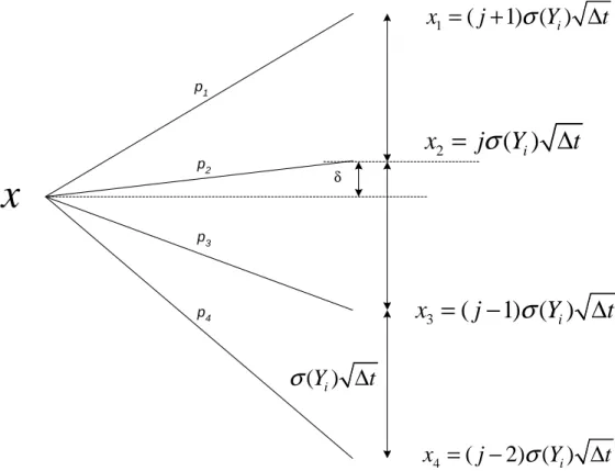
Assume we are working in the ith time step, and that we are at a point where the log stock price isx. What are the possible successors ofx?
Since we do not wish to drag the entire set of n particles Yn along the tree, which would force us to shoot offnadditional branches at each node, we propose the following way of reducing this number to one, while allowing the volatility values to change from one time step to the next in a manner consistent with the filtered particle distribution Φn
K. We simply sample a volatility value from the distribution ΦnK at each time periodih,i∈ {1,2, . . . , N}. Denote the value drawn at stepicorresponding to timeihbyYi. Corresponding to this volatility valueYi we construct the successors in the following way.
We consider a grid of points of the form lσ(Yi)
√
∆t withl taking integer values. No matter where the parentxis, it will fall at one such point or between two grid points. In this grid, letj be the integer that corresponds to the point abovex. Mathematically,jis the point that attains: infnl∈N:l σ(Yi)
√
∆t≥xo. We will have two possible cases: either the pointj σ(Yi)
√
∆ton the grid corresponding toj(above) is closer to x, or the point (j−1)σ(Yi)
√
∆t corresponding to j−1 (bellow) is closer. We will useδ to denote the distance from the parentxand the closest successor on the grid. We will use qto denote the standardized value, i.e.
q:=δ/σ(Yi)
√
∆t. (4.1)
p1 p3 δ
( )
Y
it
σ
∆
2( )
ix
=
j
σ
Y
∆
t
3(
1) ( )
ix
= −
j
σ
Y
∆
t
1(
1) ( )
ix
= +
j
σ
Y
∆
t
x
p2 p4 4(
2) ( )
ix
= −
j
σ
Y
∆
t
Figure 1: The basic successors for a given volatility value. Case 1.
Case 1. j σ(Yi)
√
∆t is the point on the grid closest tox.
Note that in this caseδis: δ=x−j σ(Yi)
√
∆t.
Remark 4.1. Withδas above andqdefined in (4.1) we haveδ∈h−σ(Yi) √ ∆t 2 ,0 i andq∈ −1 2,0
Figure 1 on page 13 refers to this case.
One of the assumptions we need to verify is (2.4), which asks the mean of the increment to converge to the drift of the process Xt in (2.2). In order to simplify this requirement, we add the drift quantity to each of the successors. This trick will simplify the conditions (2.4) to require the convergence of the mean increment to zero. This idea has been previously used by many authors including Leisen as well as Nelson & Ramaswamy.
Explicitly, we take the 4 successors to be: x1 = (j+ 1)σ(Yi) √ ∆t+r−σ2(Yi) 2 ∆t x2 =jσ(Yi) √ ∆t+r−σ 2 (Yi) 2 ∆t x3 = (j−1)σ(Yi) √ ∆t+r−σ 2 (Yi) 2 ∆t x4 = (j−2)σ(Yi) √ ∆t+r−σ2(Yi) 2 ∆t (4.2)
First notice that condition (2.6) is trivially satisfied by this choice of successors. We now define a system of equations consisting of the variance condition (2.5), and the mean condition (2.4), and we solve it for the joint probabilitiesp1,p2,p3 andp4. Because the market is incomplete, we cannot expect to have a unique
solution to the system. However, each solution will give us an equivalent martingale measure.
Algebraically, we may write: j σ(Yi)
√
∆t=x−δ, and using this we infer that the increments over the period ∆tare: x1−x =σ(Yi) √ ∆t−δ+r−σ2(Yi) 2 ∆t x2−x =−δ+ r−σ 2 (Yi) 2 ∆t x3−x =−σ(Yi) √ ∆t−δ+r−σ 2 (Yi) 2 ∆t x4−x =−2σ(Yi) √ ∆t−δ+r−σ2(Yi) 2 ∆t (4.3)
Conditions (2.4) and (2.5) translate here as:
E[∆x|Yi] = r−σ 2(Y i) 2 ∆t V[∆x|Yi] =σ2(Yi)∆t
where by ∆x we denote the increment over the period ∆t. Since ∆x given Yi is equal to xj −x with probabilitypj, forj = 1,2,3,4, we simply need to solve the following system of equations with respect to p1,p2p3 andp4: σ(Yi) √ ∆t−δp1 +(−δ)p2+ −σ(Yi) √ ∆t−δp3+ −2σ(Yi) √ ∆t−δp4= 0 σ(Yi) √ ∆t−δ 2 p1 +(−δ)2p2+ −σ(Yi) √ ∆t−δ 2 p3+ −2σ(Yi) √ ∆t−δ 2 p4 −E[∆x|Yi]2=σ2(Yi)∆t p1+p2+p3+p4= 1 . (4.4)
Eliminating the terms in the first equation of the system we get:
σ(Yi) √ ∆t(p1−p3−2p4)−δ= 0 or p1−p3−2p4= δ σ(Yi) √ ∆t. (4.5)
Neglecting the terms of the formr−σ 2
(Yi)
2
the following: σ2(Yi)∆t=σ2(Yi)∆t(p1+p3+ 4p4) + 2δσ(Yi) √ ∆t(p3−p1+ 2p4) +δ2 −σ(Yi) √ ∆t(p1−p3−2p4)−δ 2 .
After simplifications, we obtain the equation:
(p1+p3+ 4p4)−(p1−p3−2p4)2= 1.
So now the system of equations to be solved is the following: p1+p3+ 4p4= 1 + δ 2 σ2(Y i)∆t p1−p3−2p4=σ(Yδ i) √ ∆t p1+p2+p3+p4= 1 (4.6)
This system with 4 unknowns and 3 equations has an infinite number of solutions. Since we are interested in the solutions in the interval [0,1], we are able to reduce somewhat the range of the solutions. Let us denote bypthe probability of the branch furthest away from x. In this casep:=p4. Expressing the other
probabilities in term ofpand theqdefined in Remark 4.1, we obtain:
p1=12 1 +q+q2−p p2= 3p−q2 p3=12 1−q+q2−3p (4.7)
Now using the condition that every probability needs to be between 0 and 1, we solve the following three inequalities: 1 2 −1 +q+q 2 ≤p≤12 1 +q+q 2 q2 3 ≤p≤ 1+q2 3 1 6 −1−q+q2 ≤p≤16 1−q+q2 (4.8)
It is not difficult to see that the solution of the inequalities (4.8) isp∈[121,16]. Consequently, we will obtain an equivalent martingale measure for everyp∈[121,16] thanks to the first equation in (4.4).
We postpone the statement of this result until after Case 2.
Case 2. (j−1)σ(Yi)
√
∆t is the point on the grid closest tox.
In this case δ=x−(j−1)σ(Yi)
√
Remark 4.2. This case is the mirror image of the first case with respect to x. In this second case we will obtainδ∈h0,σ(Yi) √ ∆t 2 i andq∈ 0,12
The 4 successors are the same as in Case 1; the increments are calculated similarly to (4.3). Using the Remark 4.2 together with the equations (2.4) and (2.5) gives the following solution:
p2= 12 1 +q+q2 −3p p3= 3p−q2 p4= 12 1−q+q2−p , (4.9)
where p is the probability of the successor furthest away, in this case p1. This is just the solution given
in (4.7) with p1 ⇄p4 and p2 ⇄p3 taking into account the interval for δ. Thus, we are able to state the
following result.
Lemma 4.3. If we construct a one step quadrinomial tree with the successors given by (4.2), and we denote bypthe probability of the successor furthest away from x, then for everyp∈[1
12,
1
6]:
(i) in Case 1(q∈[−1
2,0])the relations (4.7)define an equivalent martingale measure.
(ii) inCase 2(q∈[0,1
2]) the relations (4.9)define an equivalent martingale measure.
Because of the indetermination on p ∈ [1
12,
1
6] in the above two lemmas, as we said, our martingale
measure is not unique. Consequently, option prices are determined only after a value ofphas been chosen, that is to say, the market defined by the one-period model, and any multiperiod constructions based on it, is incomplete. This is of course no surprise, since volatility is not directly observable in discrete time, and is not a traded asset, and therefore we have a model with two sources of randomness and only one liquid risky asset. In order to complete the market, we make the following.
Assumption 4.4. There is a liquid market for some contingent claim based onS.
The assumption of no arbitrage in itself is not sufficient to determine all option prices, but itdoes imply some consistency relations between various claim prices. With the above assumption 4.4, if we use that contingent claim as a benchmark, saying that its market prices are valid, then we can consider it as a second liquid risky asset, and the price of any other derivative onSwould be uniquely determined. In practice, one only needs to find the valuepwhich yields the best fit between any pricing scheme for the benchmark option using ourp-based one-period model, and the market price for the benchmark option. A situation where we do just this is given in Sections 4.4 and 6.
Remark 4.5. As we observed above, constructing the Equivalent Martingale Measure involves solving a system with 3 equations and 4 unknowns. It is natural to ask then, why not try a tree with three successors, which will in turn imply solving a system with 3 equations and 3 variables. However, it turs out that such
a system has no solution for any possible choice of successors. This is to be expected, since the existence of such a solution will contradict the incompleteness of the market.
4.2
Construction of the multi-period model. Option valuation.
Suppose now that we have to compute an option value. For illustrative purposes we use an European type option, but the method should work with any kind of path dependent option e.g., American, Asian, Barrier etc.
Assume that the payoff function is Φ(XT). The maturity date of the option isT, and the purpose is to compute the value of this option at timet = 0 using our model (2.2). We divide the interval [0, T] into N smaller ones of lengthh= ∆t:= T
N. At each of the pointsi∆t withi∈ {1,2, . . . , N}we then construct the successors in our tree as in the previous section. This tree converges in distribution to the solution of the stochastic model (2.2). A proof of this fact using Theorem 2.2 is found in the next subsection.
In order to calculate an estimate for the option price we employ a resampling method based on the parti-cles defining the approximate discrete distribution for the initial volatilityY. Suppose that we have the dis-crete probability distribution ofY, i.e. we know the stochastic volatility particle filter values{Y¯1,Y¯2, . . . ,Y¯n}, each with probability {p¯1,p¯2, . . . ,p¯n}. We sample N values from this distribution, and use them like the realization of volatility processY along theN levels of the tree, into the future. In other words, call these sampled valuesY1,· · ·, YN. We start with the initial valuex0. We then compute the 4 successors ofx0 as in
the previous section for the first sampled value,Y1. After this, for each one of the 4 successors we compute
their respective successors for the second sampled volatility valueY2, and so on, resulting in a quadrinomial
tree.
This tree allows us to compute one instance of the option price by using the standard pricing technique that is consistent with a no-arbitrage condition: we compute the value of the payoff function Φ at the terminal nodes of the tree; then, working backward in the path tree, we compute the value of the option at timet= 0 as the discounted expectation of the final node values using one of the martingale measures found in the previous section. Because the tree is recombining by construction, the level of computation implied is manageable, of a polynomial order in N. We will present empirical evidence of this fact in Section 6. The complexity of the filtering algorithm leading to the original particle values ¯Y :={Y¯1,Y¯2, . . . ,Y¯n} is no greater.
If we are to iterate this procedure by using repeated samples {Y¯1,· · ·,Y¯n′
}, we can take the average of all prices obtained for each tree generated using each separate sample. This Monte Carlo method converges, as the number of particlesnand the number of Monte Carlo samplesn′ increases, to the true option price
for the quadrinomial tree in which the original distribution of the volatility is the true filtered lawp0(dy) of
Y0given past observations of the stock price. We leave a full proof of this convergence out of our article. It
of samplesn′ and fixed number of time iterations K, as the number of particlesnincreases, forn′ samples {Y1,· · ·, Yn′} from the distribution of particles {Y¯1,Y¯2, . . . ,Y¯n} with probabilities{p¯1,p¯2, . . . ,p¯n}, the Yi’s are asymptotically independent and all identically distributed according to the law ofY0 given all past stock
price observations. Chapter 8, and in particular Theorem 8.3.3 in (Del Moral, 2004), can be consulted for this fact. The convergence proof in the next section is also based on del Moral’s propagation of chaos.
In fact, a more precise convergence result can be established here. According to del Moral’s propagation of chaos Theorem 8.3.3 in (Del Moral, 2004), if the number of samplesn′=n′(n) is taken to be a function
of the number of particles n, and if the number of time steps K =K(n), used before time 0 to simulate the particle approximation ofY0, is also a function ofn, then the speed at which the samples{Y1,· · ·, Yn′}
converge to independent copies of the filtered law ofY0 given all past continuously observed stock prices is
given by
|n′(n)|2K(n)
n . (4.10)
Thus if K andn′ are chosen so that the above quantity tends to 0 asntends to +∞, we indeed have the
announced convergence.
Because of the very special nature of stochastic volatility filtering, at any time t, the squared volatility in the original model (2.1) is actually equal to the differential of the quadratic variation of the martingale X, which means that when the number of time observationsK tends to infinity in a finite time interval [0, T], σ2(Y
t) does not need to be filtered: it is actually known, given the entire past of the path of X in continuous time. For simplicity, assume thatσ2 is a bijective function on the space whereY lives, or change
the dynamics ofY so that σ2(Y
t) is Yt itself. Alternately, we see that the filtered value of Y0 tends to the
actual objective value ofY0 when K tends to +∞. Hence in the above situation where we can apply the
propagation of chaos, ifK(n) also tends to +∞, we can guarantee that our sample{Y1,· · ·, YK}converges in distribution to independent copies ofY0. Then, also invoking the convergence theorem of the next section,
we conclude that the option valuation method described in this section converges to the true option price under the Static model (2.2) where the fixed random variableY is the true objective volatilityY0.
The above considerations do not preclude us from using limn→∞n′(n) =∞while the number of discrete
stock observations K remains fixed; in this case, expression (4.10) shows that, as soon as n′(n) ≪ n2, if
n→ ∞, the samples{Y1,· · ·, Yn′}converge in law to i.id. copies of the the filtered law pK(dy) ofY0 given
past discrete stock observations, which is sufficient to implement the Monte Carlo pricing method described in this section.
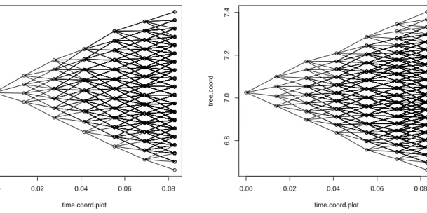
Figure 2, on page 19, contains an example of two simulated trees. We can visualize from the presented images that the trees recombine, and that the level of recombination is closer to that of a classical trinomial or binomial tree (linear growth of number of nodes for each additional time step), and accordingly the level of computation based on such a tree is not very high. Because our tree is constructed using the sampled volatility values at each time step, the number of nodes at each time depends on historical stock
0.00 0.02 0.04 0.06 0.08 6.7 6.8 6.9 7.0 7.1 7.2 7.3 time.coord.plot tree.coord
(a) One instance of the generated tree
0.00 0.02 0.04 0.06 0.08 6.8 7.0 7.2 7.4 time.coord.plot tree.coord
(b) Another instance of the generated tree Figure 2: Example of reduced trees
observations. It is therefore not predetermined, and the degree of recombination varies slightly as time increases. We present some empirical studies about the rate of increase of the total number of nodes in the tree in Section 6. The theoretical study of how much recombination actually occurs seems to be a non-trivial problem, as a consequence; we leave such a discussion out of this paper, for the sake of conciseness.
4.3
Convergence result for the quadrinomial tree
As noted in Section 2 we shall prove that our constructed tree converges to the solution of the process
dXt= r−σ 2(Y) 2 dt+σ(Y)dWt,
whereY is a random variable with the same distribution as the actual volatility process at time 0 i.e.,Y0.
Theorem 4.6. Consider the quadrinomial tree, with nodes indexed by the log values of a stock, defined by the successors x1, x2, x3, x4 of a value x as in (4.2), with probabilities p1, p2, p3, p4 given by the relations
(4.7) (resp. (4.9)), with p = p1 (resp. p =p4) when x1 is furthest from the parent value x (resp. x4 is
furthest). For any fixedp∈[121,16], these probabilities define a martingale measure on the paths of the tree. Furthermore, the Markov chain defined on the vertices of the tree under any such measure on the tree, defined by the relations (4.7)and (4.9), converges in distribution to the continuous process (2.2)as the time interval
Proof. The first equation in the systems we solved above guarantees that the discounted process has expected increments zero, thus assuring us that the resulting measure we find is a martingale measure.
It remains to show the convergence result, and to this end we are using Theorem 2.2. More specifically, we are going to prove that the two critical assumptions (2.4) and (2.5) are satisfied. Assume that at step ithe tree is constructed using the volatility value Yi sampled from the distributionYn. The probability of this outcome is denoted with ¯pi. We remind the reader that the formulae for these quantities are given in (3.6).
Let us define the variableX in Case 1:
X = σ(Yi) √ ∆t−δ with probability p1 ¯ pi −δ with probability p2 ¯ pi −σ(Yi) √ ∆t−δ with probability p3 ¯ pi −2σ(Yi) √ ∆t−δ with probability p4 ¯ pi
and inCase 2as:
X = 2σ(Yi) √ ∆t−δ with probability p1 ¯ pi σ(Yi) √ ∆t−δ with probability p2 ¯ pi −δ with probability p3 ¯ pi −σ(Yi) √ ∆t−δ with probability p4 ¯ pi where δ σ(Yi) √ ∆t is in the interval [− 1 2,0] in case 1 and in [0, 1 2] in the case 2.
Let us note here that using Lemma 4.3 and the equations (4.7) and (4.9) the probabilities defined above are symmetrical with respect toxand that in either of the two cases ∆x|Yi =X+
r−σ 2 (Yi) 2 ∆t. Also, note that the system (4.4) gives the mean and variance ofX as 0 andσ2(Y
i)∆t, respectively. Thus, we have:
E[∆x|Yi] =E[X] + r−σ 2(Y i) 2 ∆t = r−σ 2(Y i) 2 ∆t
Now from the definition ofbh(x) we have:
bh(x) = E[∆x|Yi] ∆t =r− σ2(Y i) 2
At this point we need to invoke Theorem 8.3.3 in (Del Moral, 2004). When applied to our particular case it implies that each of the variablesY1,Y2,. . . drawn from the discrete distributionYnconverge in distribution
prices before time 0. Moreover, using the facts given in the last paragraph of the previous subsection, when ∆t →0, the law ofY∆ttends to the law of the actual initial volatilityY
0. Thus for a nlarge enough and
∆t small enough, using the continuity ofσ(y), we obtain that Assumption (2.4) is satisfied. SinceVar[∆x|Yi] =Var[X] we have:
E[(∆x)2|Yi] =Var[X] +E[∆x|Yi]2=σ2(Yi)∆t+ r−σ 2(Y i) 2 2 ∆t2 Thus: ah(x) = E[∆x2|Y i] ∆t =σ 2(Y i) + r−σ 2(Y i) 2 2 ∆t
Using the fact thatris a constant and that the functionσ is locally bounded, the second term inah(x) converges to 0 as ∆t→ 0. Using again the Theorem 8.3.3 in (Del Moral, 2004) and the continuity of the functionσ2(y), for a large enoughn, we obtain the Assumption (2.5).
4.4
Practical issues; choosing
p
To construct our tree we need to know the value of the parameterpdescribed in the previous subsections. In order to do that we use the price of a suitably chosen option from the market to calibrate for the parameter p. The option we chose to use in our numerics (see Section 6) is the previous day (April 21, 2004, in the case of the S&P500, and July 18, 2005 for IBM) at-the-money option, but theoretically, it could be any option from any moment in the past. For fixed values ofpon a dense grid on the interval [121,16] we generate trees and compute option prices corresponding to eachpin the grid. Then we compare the results obtained with the price of the option from the market and we choose the valuepthat gave the closest value to the option on the market.
We use this parameterpto compute values for all the options at time 0 (April 22, 2004, and July 19, 2005 respectively). A graphical illustration of this process applied to a specific example is presented in Figure 4. It turns out that these option prices are quite insensitive to the actual choice of p, for pin a wide range within the interval [1
12,
1
6]. This robustness is a highly desirable property when one is faced with deciding in
a rather arbitrary way how to choose a martingale measure.
byCthe value of the option obtained using our tree method, we can compute: delta=∂C ∂S = C(S+ ∆S)−C(S−∆S) 2∆S gamma=∂ 2C ∂S2 = C(S+ ∆S)−2C(S) +C(S−∆S) ∆S2 theta=∂C ∂t = C(t+ ∆t)−C(t) ∆t rho=∂C ∂r = C(r+ ∆r)−C(r) ∆r
Here the value of the option is calculated using various initial conditions. For example, C(S + ∆S) is estimated using an initial asset price ofS+ ∆S with ∆S small. ∆S= 0.001S would be a good choice here. Every price in a difference or a sum should be computed using the same set of volatility values to eliminate variability due to Monte Carlo randomness.
Notice that we do not compute vega which is the derivative with respect to the volatility, because in our case it has no clear interpretation. We could also compute a nonstandard derivative with respect to the above described parameter p.
5
The Dynamic Model: using stochastic volatility filtering in a
Monte Carlo method
The idea of this model is to start with the estimated volatility distributionY0n := ΦnK at the present time, represented by its weighted particles Yn = ¯
Yj,p¯j:j= 1,· · ·, n and with the logarithm of the price of the stock today x0 = logS0 in equation (2.1), and then to take advantage of the same particle filtering
scheme we used in the Section 3 to generate future stock prices and volatility values: that is to say, we wish to use stochastic volatility filtering in a dynamic way for pricing.
More precisely we start with x0 and the Y0n distribution. We sample a volatility value y0 from the
empirical distribution Yn
0. We divide the time to expiration T into N intervals of length ∆t =T /N and
generate a path (X, Y) recursively:
Y(y0)i+1:=Yi+1=Yi+α(ν−Yi)∆t+ψ(Yi)Ui √ ∆t, X(x0)i+1:=Xi+1=Xi+ (r− σ2(Y i) 2 )∆t+σ(Yi)U ′ i √ ∆t. (5.1)
where the variablesUi andUi′ are iid standard normal andi∈ {0,1,2, . . . , N−1}. In other words, we use the actual “Stochastic Volatility” dynamics for simulating future values of (X, Y), but using the risk-free rate for the mean rate of return of the simulated stock in (5.1), and started from a sample from the initial distributionδ{x0}⊗Y
n
must be consistent with sampling from a martingale measure, since we are doing pricing via risk-neutral valuation.
Once we find the value at the expiration X(x0)N = XT we can compute the value of the option at the expiration, and then we discount back to the present value using the risk-free rate. This represents one replication of a Monte Carlo method: to compute an estimate of the option price we generate many replications (typically of the ordern′′= 106) then compute the average of the values obtained. This average
is our estimate for the price of the option today. The convergence, and the convergence speed, of order (n′′)−1/2
, is of course guaranteed by a standard argument based on the central limit theorem. We omit the details.
Any straight Monte Carlo method is notoriously inefficient, and one may try to improve the convergence of the method by such techniques as reduction of variance, and the like. However, since our dynamic model yields option prices which are not as close to those given in the market as the static model’s prices, there seems little reason to improve the efficiency of our Monte Carlo method for the dynamic model.
At this stage it is worth noting that this article’s second-named author, in (Viens, 2002), provides a Monte Carlo method that solves a related stochastic portfolio optimization problem using elements of stochastic control, dynamically in time, based on the dynamic evolution of the stochastic volatility particle filter. Because of the non-linear nature of portfolio optimization, as opposed to the linear nature of option pricing, the numerics proposed in (Viens, 2002) are difficult to implement in general (see however the special case of power utility, for which a successful implementation can be found in (Batalova et al., 2006)).
We hope that the successful option-pricing implementation in the present article will be an invitation for researchers to apply the same models and methods to the optimization problem in (Viens, 2002).
6
Using real data: European Call options on S&P500 and IBM
We have chosen to illustrate our method with two sets of data. The first set is S&P500 stock and call option data gathered on April 21-22, 2004. We are using daily data from January 1st, 1999 to April 21, 2004 to compute the discrete volatility distribution according to the method described in Section 3. The second dataset used is IBM stock and call option data gathered on July 18-19, 2005. We present a more detailed explanation about this dataset on page 25.
We are working with the model presented in (2.1) with φ(y) =β andσ(y) =e−|y|, using the following
parameters for the volatility equation: α = 50, m = −4.38, β = 1, and µ = 0.04 for the price. The parameters have been estimated from the data, and the short term interest rater= 0.01 used for the tree construction is the value published for April 21, 2004.
We estimate the discrete volatility distribution using the Del Moral, Jacod, Protter method presented in Section 3. We used m= 300 time steps between any two observations, and n = 1000 mutation particles.
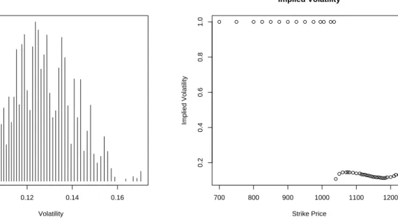
Figure 3 (a) presents a plot of this estimated distribution using the final 1000 particles. 0.10 0.12 0.14 0.16 0.00 0.01 0.02 0.03 0.04 Volatility Probability
(a) Estimated discrete Volatility Distribution
700 800 900 1000 1100 1200 0.2 0.4 0.6 0.8 1.0 Implied Volatility Strike Price Implied Volatility (b) Implied Volatility Figure 3: Estimates from historical data
To compare our method, we also estimate the implied volatility on April 21 for a range of strike prices from the option data available that day. To do so, we use a simple bisection method. Figure 3(b) shows the implied volatility’s behavior for various strike prices.
We should note that we used the option and stock (index) data available on April 21st to estimate these two plots. The implied volatility Figure 3(b) corresponds to the 29-day-maturity options but it is representative for the other maturities as well. We notice very high implied volatility values for options deep in the money, and for most others the implied volatility is around 0.12−0.135.
Using the data available a day earlier we estimate option prices for that day for many values of the parameterpin the interval [121,16]. Then, we compare the estimated prices with the price of the “benchmark option” which we chose to be the option at the money. We can see computed values corresponding to a grid for thepparameter in Figure 4.
Beginning withp= 0.135 and ending with p= 0.16, the option values obtained are close to each other. In fact, this is a feature we have observed for all the option values calculated for the entire range of strike prices. The values of the 29-day-maturity options obtained for p = 0.135 are presented in Table 1 in the Appendix.
For better illustration of the performance of the various methods we present in Figures 5 and 6 on pages 34 and 35, the values of the options separated in groups depending on the range of the strike prices (at the money, and out of the money, respectively).
0.09 0.10 0.11 0.12 0.13 0.14 0.15 0.16 −1500 −1000 −500 0 p Option Value
(a) All the values
0.12 0.13 0.14 0.15 0.16 15.8 15.9 16.0 p[7:15] Option Value (b) Zoomed in figure Figure 4: Determining optimal p parameter value
We mention that the plot of the deep-in-the-money options is not shown since the intrinsic value of the options dominate all the valuations methods and no method performs better than the rest. We could also observe the option values at the top of Table 1 for this fact.
All the above option-price graphs include, for comparison, the bid-ask spread of the actual prices seen on the option market, and the price given via the standard Black-Scholes formula with constant (non-random) volatility.
One of the advantages of our method is that it allows the computation of option prices even when there exists no formula for that option type. This idea is even applicable to standard vanilla options, in the following situation. In the third Friday of each month the European option with maturity that month expires. Thus the option with expiration 2 months becomes a one month option and so on. Also, during the following Monday and Tuesday an option with a new, intermediate, maturity date is starting to be traded. Since there is no implied volatility in the previous day for this option we suspected that our method will perform well.
For this simulation we use IBM stock data from July 18-19, 2005. The new options with expiration in September did not appear until Tuesday July 19, 2005 so we are using the Monday July 18 for volatility calibration and finding the optimalpaccording to the method described above. The coefficients used in this case were: α= 11.85566,ν = 0.9345938β= 4.13415,µ= 0.04588, andr=.0343. We have estimated these coefficients from the historical data, the method we used is to be the subject of another article.
36.
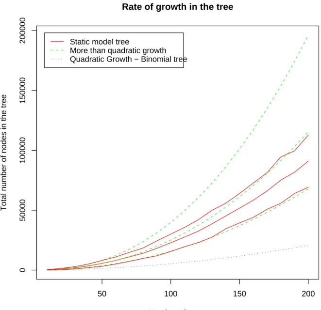
Discussion about the rate of growth in the tree
As pointed out by our anonymous referees a discussion about the recombination level of the constructed trees would be beneficial to justify the utility of the method. We have empirically studied this problem for the trees created to evaluate the IBM at the money option (Strike price =80). We present a plot of the evolution of the total number of nodes in the generated tree in Figure 8 on page 37. On thex-axis we plot the number of steps in the tree. As we see in the plot our tree model contains more nodes than the classical Binomial tree (n(n+ 1)/2∼O(n2)), but it is comparable with a polynomial inn. In fact the curve produced
forn3 is much higher and Figure 8 shows that within 3 standard deviations our node growth rate is clearly
bellown2.3, indicating that a typical tree is quite manageable.
We will note however that the total number of nodes is dependent on the original distribution of the volatilityY. A theoretical result relating these two quantities would be extremely valuable but beyond the scope of the present article.
Discussion about the sensitivity of the estimation with respect to the number of
steps in the tree
It is also interesting to see how the precision of our tree estimate changes when increasing the number of steps in the tree and the number of generated trees. Once again we looked at the IBM at-the-money option. We generated the estimate varying first the number of time steps in the tree and second the number of generated trees. More specifically, assume that each estimate comes from a distribution with meanµ and standard deviation σ. We already know from the convergence Theorem 4.6 thatµis the true value of the option. We want to estimate σ and for this purpose denote the number of steps in the tree by nand the number of simulated paths byN. Assume thatX1=X1(n), X2 =X2(n),· · ·, XN =XN(n) are the values obtained from each simulated path, we can then estimate σas:
ˆ σ(N)2= 1 N−1 N X i=1 (Xi−X)¯ 2
We wanted to study what happens with this estimate when we changen andN. We did just that and we plotted the results in Figure 9 on page 38. Part (a) of the plot keeps N = 100 constant and varies n. We can see that ˆσdecreases as the number of steps in the tree increases, which is to be expected. Part (b) keepsn= 100 constant and variesN. We can see that ˆσstays approximately constant, this is natural since the value it estimates does not depend onN.
current plots are more enlightening.
7
Conclusions
This article implements a new way of pricing options under stochastic volatility, by taking advantage of an optimal stochastic particle filtering algorithm yielding the probability distribution of the present-day volatility based on past stock observations. The particles of this filter are used in conjunction with a highly recombining quadrinomial tree for pricing options, based on standard arbitrage-free methodology under a martingale measure which is determined, in this incomplete market, by choosing a benchmark option. The approximation methods presented in this work are computationally intensive, but are based on simple algorithms featuring low, manageable, complexity. The option prices based on our quadrinomial tree implementation are very close to the same prices observed on the option market.
The two numerical cases presented here are fundamentally different. In the first application we used an Index (S&P 500) which is not very sensitive to small movements in the market. For the second application we choose a popular technology stock, IBM; we observed our same basic conclusions for many other stocks (Microsoft, Intel, Yahoo, Ford and GM), not included here for obvious space considerations.
In the case of the S&P 500 we observe that pricing using our Static model (Section 4) is clearly better than the pricing using the Dynamic model of Section 5, since the former typically falls within the option market’s bid-ask spread, while the latter does not. This is despite the fact that the Dynamic model approximates pricing under the true Stochastic Volatility model, while in the Static model, volatility is assumed to be constantly distributed in the future according to its best present estimated distribution given all past stock price observations.
In addition to the heuristic explanation given at the end of the introduction (on page 4), by which the static model is closer to what practitioners are actually doing when adjusting the Black-Scholes formula to account for non-constant volatility, there is a numerical reason for its superiority over the dynamical model, which became evident to us after we studied the total number of nodes in the constructed trees. For the static model we have used trees with 100 steps and we replicated the trees 100 times. We suspected that we were using a large number of computations and to make sure that we do not give an unfair advantage to the static model we used 100 time steps in the Dynamic model but with 100,000 simulations of the path. This is apparently not a sufficiently large number for the Monte Carlo computations. After we studied the number of calculations in the tree we discovered that for a 100 steps tree the average total number of nodes is around 22,000. If we do a simple calculation we observe that the number of computations for the Static model is about 44·105 (we have to go twice through the trees) versus∼100·105 for the Dynamic model.
This fact also explains why the run time for the Dynamic model is much larger than the run time for the Static model.
If we look at the three regions depending on how close the strike price is to the stock price in that respective day, we see that the best performance is obtained for the options at-the-money – conveniently so, since those are the majority of options traded. We suspect that we have obtained better results for that region because we used an option at the money to calibrate the parameter p which defines our choice of martingale measure. This fact would suggest to use different optimal values ofpfor each of the three regions. Recalibratingpfor each maturity date should provide even better estimates, although this might go against the idea of arbitrage-free consistency within a single option market.
On the other hand, since we are using European call options, for which there exists a formula that every market participant can readily use at any moment, our results are naturally not far from the values obtained using the Black-Scholes formula. The strength of our method is that it works for any type of option including those that do not have a valuation formula, and may be path dependent.
This fact is illustrated in the second analysis (the IBM case). We see that the Static model once again performs better for at the money options (in the Strike price range 75-85). In this case we also wanted to investigate the reason why the Dynamic method performed worse in the previous simulation so we increased the number of simulations by 100 (thus now using 108 runs). We see that there is no detectible difference
now between the Static and the Dynamic models, with the exception of the runtime, which naturally is huge now for the Dynamic model when compared with the Static one.
In conclusion, this article’s merit is in showing that in a well-known and mature market, our quadrinomial tree method outperforms others techniques, including the classical Black-Scholes method, or the Monte Carlo method for the Stochastic Volatility model, even when the latter is based on an excellent particle approximation of the best possible stochastic volatility estimation technique.
Lastly, we mention the question of hedging. Since we can estimate the sensitivity of the estimated option price with respect to the various factors in the model (the Greeks: delta, gamma, theta and rho) we can do a heuristicdelta hedging: starting with the option value at time zero, we can devise a dynamic trading strategy in stock and in a risk-free asset, based on the dynamically observed values of the option’s delta (for example), that approximately replicates the payoff of the option at maturity. We will investigate this topic in separate publication.
8
Appendix
Strike Price Bid-Ask Spread Implied Volatil-ity Black-Scholes with const. vol = 0.13 Black-Scholes with vol = prev. day Static Tree Method Dynamic Method 700 435.9 437.9 0.99999994 440.4859435 444.7013928 440.8361291 441.6392171 750 386 388 0.99999994 390.5256538 398.3150305 390.8360651 389.4179381 800 336 338 0.99999994 340.565364 353.829711 340.8361125 343.1698244 825 311.1 313.1 0.99999994 315.5852191 332.4452883 315.8360728 317.7046472 850 286.1 288.1 0.99999994 290.6050743 311.7044205 290.8359979 288.6177766 875 261.1 263.1 0.99999994 265.6249294 291.6546932 265.8360605 264.3557368 900 236.2 238.2 0.99999994 240.6447845 272.3377894 240.8361814 242.4258073 925 211.3 213.3 0.99999994 215.6646397 253.7888212 215.8361042 216.070995 950 186.4 188.4 0.99999994 190.6844968 236.035902 190.8361121 191.9580826 975 161.5 163.5 0.99999994 165.7044244 219.0999491 165.8361814 165.3575168 995 141.7 143.7 0.99999994 145.7211165 206.1488679 145.8365447 144.0436024 1005 131.9 133.9 0.99999994 135.7308655 199.8740407 135.8375831 136.3773022 1025 112.2 114.2 0.99999994 115.7639408 187.726882 115.8489649 115.8511543 1035 102.5 104.5 0.99999994 105.8005096 181.8544762 105.1462257 104.9907379 1040 97.6 99.6 0.107155383 100.8298139 100.7659808 100.6728878 101.2075435 1050 88 90 0.135827243 90.92671721 90.98844738 91.05013255 90.85553399 1060 78.5 80.5 0.144771874 81.10857475 81.41030081 81.09046311 79.87881581 1070 69.1 71.1 0.145104229 71.4350287 71.91279678 71.32386 72.79518986 1075 64.5 66.5 0.14579457 66.67796494 67.28775275 66.42264828 64.8763511 1080 59.9 61.9 0.144722283 61.99094358 62.66457473 61.05169626 64.4851441 1090 51 53 0.142792165 52.88699128 53.67984581 52.64029526 54.52657424 1100 42.4 44.4 0.1389274 44.25484143 44.96209243 43.86203883 44.96215623 1110 34.3 36.3 0.138166845 36.23617352 37.02984103 35.8019852 38.1543003 1115 30.4 32.4 0.133875668 32.50000074 32.90619896 32.01309525 33.06596175 1120 26.7 28.7 0.131962717 28.96654938 29.1865849 28.47139516 31.31540725 1125 24 24.7 0.131792247 25.64879123 25.86109624 25.12064397 26.1069527 1130 20.5 22 0.127446949 22.55710072 22.24252051 21.93006175 24.08772635