Developing Physician Migration
Estimates for Workforce Models
George M. Holmes
and Erin P. Fraher
Objective. To understand factors affecting specialty heterogeneity in physician
migra-tion.
Data Sources/Study Setting. Physicians in the 2009 American Medical Association
Masterfile data were matched to those in the 2013file. Office locations were geocoded in both years to one of 293 areas of the country. Estimated utilization, calculated for each specialty, was used as the primary predictor of migration. Physician characteristics (e.g., specialty, age, sex) were obtained from the 2009file. Area characteristics and other factors influencing physician migration (e.g., rurality, presence of teaching hospi-tal) were obtained from various sources.
Study Design. We modeled physician location decisions as a two-part process: First,
the physician decides whether to move. Second, conditional on moving, a conditional logit model estimates the probability a physician moved to a particular area. Separate models were estimated by specialty and whether the physician was a resident.
Principal Findings. Results differed between specialties and according to whether
the physician was a resident in 2009, indicating heterogeneity in responsiveness to poli-cies. Physician migration was higher between geographically proximate states with higher utilization for that specialty.
Conclusions. Models can be used to estimate specialty-specific migration patterns for
more accurate workforce modeling, including simulations to model the effect of policy changes.
Key Words. Workforce, physician migration, conditional logit, simulation
There is a lack of consensus on whether the nation will have enough physi-cians to meet the rising demand from health care services, with some arguing that a physician shortage will develop (AAMC 2015), and others arguing that supply will be sufficient (Salsberg 2015). Although there is disagreement on whether there is sufficientaggregatesupply, it is generally accepted that we cur-rently have and will continue to have amaldistribution of physicians (Eden, Berwick, and Wilensky 2014). The problem of physician maldistribution is a long-standing one and exists despite the fact that the physician workforce is a
©Health Research and Educational Trust
DOI: 10.1111/1475-6773.12656
THE EVOLVING U.S. HEALTH WORKFORCE
529
mobile one. Previous studies have shown that one in five physicians change their county of practice within a 5-year period (Ricketts 2013a, b) and that rural areas, especially those on the fringes of urban ones, often gain physicians as a result of these moves (Ricketts and Randolph 2007).
Seminal work by Newhouse offered the“sandpile”hypothesis—supply will be higher in more populous areas with more demand, and then as the overall supply increases, supply in areas with lower demand will increase (Rosenthal, Zaslavsky, and Newhouse 2005). In his work, and most subse-quent work, the demand for physician services and physicians’location deci-sions was driven by population growth and demographic factors, including the overall wealth of the community (Cooper, Getzen, and Laud 2003). Other research on physician migration patterns has identified additional factors driv-ing location behavior, includdriv-ing the effect of the federal programs such as the National Health Service Corps (Pathman et al. 2012) and the importance of medical school and residency training location on physicians’practice loca-tion (Rosenblatt et al. 1993, 2002; Phillips et al. 2009; Chen et al. 2010). Stud-ies of the effect of individual-level physician characteristics on physician migration have shown that younger, female physicians tend to move more than older, male physicians and that primary care physicians and general sur-geons less than other specialties (Ricketts 2013a, b).
Studies of the effect of physician specialty on migration suggest that more specialized physicians move more than generalists (Ricketts 2010, 2013a, b). This work suggests these moves may be the result of a physician’s decision to locate to communities with higher population densities and aca-demic health centers where more specialized practice is economically feasible. However, these studies leave important gaps in knowledge. In general, they do not specifically identify how the market for physician services may vary across specialties (e.g., family medicine vs. pediatric neurosurgeon) and between geographic areas. Models that examine the demand for specific types of health services at a more granular geographic level than state are needed to account for variations in demand for different types of physicians in different labor markets.
The health care system is undergoing a period of rapid transformation in response to the Affordable Care Act and new payment models that emphasize value over volume. State and federal policy makers are attempting to redesign graduate medical education to address physician supply and maldistribution (Spero et al. 2013; Institute of Medicine 2014; Kaufman and Alfero 2015). At the same time, market forces (e.g., the continued expansion of new models of care such as accountable care organizations and consolidation of the health care system) are changing incentives. Together, these forces lead to uncer-tainty in a period where health workforce planning is becoming more important.
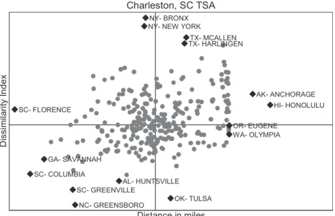
Most physician projection models do not account for the migration of physicians between or within states (Health Resources and Services Adminis-tration 2014; IHS, Inc. 2015). These models limit our ability to understand how the supply of physicians in different specialties may change over time. Such data are critical to inform policy makers’efforts to target federal funds to address physician maldistribution. Forecasts of physician supply at the national level tell us little about where, for example, we may need to invest in additional graduate medical training opportunities, increase National Health Service Corps funding, or target bonus payments. In this manuscript, we address these gaps by developing a model that specifies how individual physi-cian location decisions are influenced by the demand for services offered by that type of physician specialty at the substate level. Furthermore, we include factors not previously considered such as how well a“dissimilarity index”—a measure of how similar two locations are to each other—explains physician moves.
D
ATA
The primary independent variable is the number of visits to this spe-cialty predicted to be demanded by residents of the area. The approach is lar-gely consistent with work by others (Glied and Ma 2015). Briefly, we use Medical Expenditure Panel Survey data on national utilization patterns as a function of individual characteristics such as age, sex, insurance coverage, presence of comorbidities, insurance coverage, income, and health behaviors and risk factors and interpolate utilization at the local (county) level using small area estimation methods (Rao 2003). These are done for each of 19 clini-cal service areas for inpatient, outpatient, and emergency department settings. Thus, we have local (county-level) estimates for 57 different services. These are mapped into 35 different specialties using patterns of which type of spe-cialty provides for which type of services (Holmes et al. 2013). We hypothe-size that areas with higher utilization will be more attractive to physicians and thus have higher probability.
We include other measures of the area hypothesized to affect migra-tion. County sociodemographics, such as including population density, age structure (percent aged <18 and percent aged >65), economics (percent with income <US$ 50,000; percent unemployment), race/ethnicity (per-cent Hispanic; per(per-cent non-white non-Hispanic), and education (per(per-cent with at least a college degree), capture the relative appeal of the area. Because certain specialties may cluster together at a limited number of hospitals, we also include an indicator for whether there is a teaching hos-pital in the TSA (American Hoshos-pital Association), with the expectation that subspecialties would be more likely to locate in a TSA with a teaching hospital. Because (relative) physician supply tends to be lower in rural areas, we include measures for the percent of the population in the TSA living in a metropolitan and percent living in micropolitan area (US Office of Management and Budget). In our particular data extract, we did not have information on whether the physician was an international medical graduate (IMG), who are known to have different migration patterns (e.g., more likely to practice in medically underserved areas, such as being employed by city or county governments) (Cohen 2006).
Harlingen TX, or Manhattan, NY. It draws loosely from the “intervening opportunity”theory of migration (Stouffer 1940) if the“dissimilarity index” can be used as a measure of“the number of opportunities at that location.” That is, the index can be used to measure labor market opportunity (e.g., a physician specializing or interested in certain populations) as well as the desir-ability of the community; a physician practicing in a coastal South Atlantic affluent community may consider moving to a low-income Midwestern com-munity, but she may be more likely to consider a community similar to her current one. We hypothesize that moves will be more likely among similar communities, but it is also possible that physicians may look for“fresh start” and choose a dissimilar location.
The intervening opportunity theory also predicts that the probability of moving to a location will be inversely proportional to the number of more proximate opportunities; here, we use distance to approximate this notion. For each TSA-TSA dyad, we also calculate the natural logarithm of the aerial distance (in miles) between the population centroids because migration may be higher between more proximal TSAs. That is, physicians may execute a local move to a contiguous TSA within a metropolitan area, but a move across the country is more involved.
C
ONCEPTUAL
M
ODEL
Following earlier work on physician migration (Holmes 2005), we specify migration as a physician-level model involving multiple decisions. This speci-fication, rather than modeling aggregateflows, allows modeling of how physi-cian characteristics affect decisions. We specify the location as a two-decision process.
•
Decision 1: Does the physician move to a new location?•
Decision 2: If the physician decides to move, to which location does she move?current location = 292), the number of observations increases quickly (Table 1).
Given known differences in behavior of residents versus nonresidents (Ricketts and Randolph 2007), we model physicians who are in a residency program in thefirst time period separately from those who had completed res-idency prior to thefirst period. Due to space limitations, we primarily focus on those physicians who were not residents in 2009. Likewise, because physicians of different specialties have different markets and migrate in different manners (Ricketts and Randolph 2007), we model each specialty separately. Here, we focus on a subset of our 35 physician specialties, including primary care (fam-ily medicine, internal medicine, pediatrics), medical subspecialties (cardiolo-gist, pediatric nonsurgical subspecialties), and surgical (general surgery, OB/ GYN).
Move Decision
We use a logistic regression to model the probability that a physician remains in the same TSA in 2013 as in 2009. We include physician characteristics (sex, age) as well as characteristics of the 2009 area, including total demand, demand per physician, sociodemographics, rural–urban measures, and whether there is at least one teaching hospital in the TSA. We hypothesize that physicians are more likely to remain in areas with (1) higher total and (2) per-physician demand, (3) higher socioeconomic status, (4) rural communities, and (5) at least one teaching hospital. Ricketts and Randolph (2007) showed a
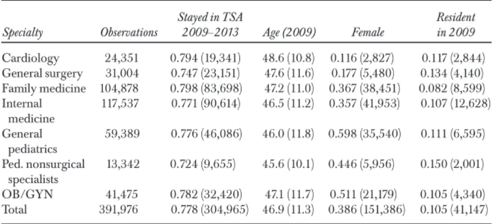
Table 1: Summary Statistics for Physician Characteristics
Specialty Observations
Stayed in TSA
2009–2013 Age (2009) Female
Resident in 2009
Cardiology 24,351 0.794 (19,341) 48.6 (10.8) 0.116 (2,827) 0.117 (2,844)
General surgery 31,004 0.747 (23,151) 47.6 (11.6) 0.177 (5,480) 0.134 (4,140)
Family medicine 104,878 0.798 (83,698) 47.2 (11.0) 0.367 (38,451) 0.082 (8,599)
Internal medicine
117,537 0.771 (90,614) 46.5 (11.2) 0.357 (41,953) 0.107 (12,628)
General pediatrics
59,389 0.776 (46,086) 46.0 (11.8) 0.598 (35,540) 0.111 (6,595)
Ped. nonsurgical specialists
13,342 0.724 (9,655) 45.6 (10.1) 0.446 (5,956) 0.150 (2,001)
OB/GYN 41,475 0.782 (32,420) 47.1 (11.7) 0.511 (21,179) 0.105 (4,340)
Total 391,976 0.778 (304,965) 46.9 (11.3) 0.386 (151,386) 0.105 (41,147)
netflow of physicians from urban to rural areas, and a teaching hospital may serve as an additional “professional magnet” encouraging physicians to remain in the community.
Location Decision
Conditional on deciding to move, the physician’s probability of selecting area A is specified as
Prðmove to AÞ ¼PexpðXAbÞ jexpðXjbÞ
where the denominator includes the sum of all areas other than the current location (given that the physician decided to move). The vectorXAcontains area characteristics known or hypothesized to affect physician migration pat-terns measured at the potential destination (rather than the 2009 location). We include the demand measures for the area, the community measures used in the“stay”model, and the dyad comparisons (dissimilarity and distance).
By combining the two results, we can generate physician-specific esti-mates of probability of migration to each TSA in the country as a function of physician and area characteristics. For example, the probability of moving from area A to area B is
PrðLocation B in2013jLocation A in2009Þ ¼Prðleave AÞ ðprðBjleave AÞ
R
ESULTS
Table 2 summarizes the physician characteristics for each of the considered cialties. The percentage of physicians staying in their 2009 TSA varies by spe-cialty, with pediatric nonsurgical specialties the least likely to remain in their location (72.4 percent) and internists the most likely to remain (79.8 percent). The average age is between 45 and 49, but the percent female varies considerably, with 11.6 of surgeons and 59.8 percent of pediatricians being female.
T able 2: Logistic R esults: D ecision to Stay in 2 0 0 9 TSA Card . Surgery F am .Med . Int .Med . P edia trics P ed .Nonsu rgeon O B /G Y N U
tilization Visits(/
TSAs in the Carolinas—Greensboro, NC, and Greenville, SC—but also Huntsville, AL, and Tulsa, OK. Meanwhile, the closest TSA—Florence, SC— has a dissimilarity index higher than the median. Consistent with Tobler’s First law of Geography (“near things are more related than distant things”), proxi-mate TSAs are more similar, but there is considerable variation: It is possible tofind near TSAs that are dissimilar and distant ones that are similar.
Regression Results: Stay
Table 3 shows the results of the logits predicting whether the physician remains in the 2009 TSA. In terms of characteristics of the current location, the higher the expected number of visits, the more likely the physician remains in that location; this variable was more predictive of staying than an aggregate population measure (based on log-likelihoods, not shown). How-ever, the more visits per physician, thelesslikely the physician remains in that location. This was unexpected, as we expected that holding constant the num-ber of visits, a higher demand per physician would mean more enticement to stay. Across the specialties, age has an increasing but diminishing effect; see Figure 2 for the probability of staying in the same TSA over 5 years for four
SC- FLORENCE
SC- COLUMBIA GA- SAVANNAH
SC- GREENVILLE
NC- GREENSBORO AL- HUNTSVILLE
NY- NEW YORK NY- BRONX
OK- TULSA TX- HARLINGENTX- MCALLEN
OR- EUGENE WA- OLYMPIA
AK- ANCHORAGE HI- HONOLULU
D
issi
mi
la
ri
ty
I
n
d
e
x
Distance in miles
T able 3: C ondition al Logit R esults: Location, Conditional on M oving Card . Surgery F am .Med . Int .M ed . P ediatrics P ed .Nonsu rgeon O B /G Y N U tilization meas ures V isits (1 0K) 1. 0 3 †(1 .0 3, 1. 0 3 ) 1.0 7 †(1 .0 7, 1. 0 8 ) 1.00 †(1 .00, 1.00) 1. 0 2 †(1 .0 2, 1. 0 2 ) 1.0 1 †(1 .0 1, 1. 01 ) 1.0 6 †(1 .0 6, 1. 07 ) 1.0 2 †(1 .0 2, 1. 0 2 ) D emand per phys (1 00s) 0.9 4 †(0.9 3, 0.9 5) 0.8 0 †(0.7 8, 0.8 3) 0.9 7 †(0.9 6, 0.9 7) 0.8 5 †(0.8 4, 0.8 6) 0.9 6 †(0.9 6, 0.9 7) 0.9 6 †(0.9 6, 0.9 7) 0.8 9 †(0.8 8, 0.9 1) D estin ation characteristics Pct childr en 1. 2 4 †(1 .1 5, 1. 3 4 ) 1.22 †(1 .1 4, 1. 3 0 ) 1. 14 †(1 .11 ,1.19 ) 1.1 5 †(1 .11, 1. 18 ) 1. 18 †(1 .1 2, 1. 2 3 ) 1.2 7 †(1 .1 6, 1. 3 9 ) 1. 12 †(1 .0 6, 1. 19 ) Pct elde rly 1. 2 0 †(1 .1 2, 1. 3 0 ) 1. 17 †(1 .1 0, 1. 2 4 ) 1. 16 †(1 .1 2, 1. 2 0 ) 1. 10 †(1 .0 6, 1. 13 ) 1.2 4 †(1 .1 8, 1. 2 9 ) 1.2 4 †(1 .1 3, 1. 3 6 ) 1. 15 †(1 .0 9, 1. 21 ) Pct w hite N on-Hispan ic 0.8 7 † (0.8 1, 0.9 4) 0.9 0 † (0.8 5, 0.9 5) 0.8 6 † (0.8 3, 0.8 9) 0.8 2 † (0.8 0, 0.8 5) 0.8 5 † (0.8 2, 0.8 9) 0.8 2 † (0.7 5, 0.8 9) 0.9 1 † (0.8 7, 0.9 6) Pct His panic 0.9 8 (0.9 1, 1. 0 4 ) 1.0 1 (0.9 6, 1. 0 6 ) 1.00 (0.9 7, 1. 0 2 ) 1.0 3 ‡ (1 .00, 1. 0 6 ) 1.0 2 (0.9 9, 1. 0 6 ) 0.9 9 (0.9 2, 1. 07 ) 1.0 7 † (1 .0 2, 1. 12 ) Pct incom e < $5 0K 0.9 2 ‡ (0.8 6, 0.9 9) 0.8 7 † (0.8 2, 0.9 2) 0.8 3 † (0.8 1, 0.8 6) 0.8 7 † (0.8 4, 0.9 0) 0.8 3 † (0.8 0, 0.8 7) 0.8 0 † (0.7 3, 0.8 7) 0.8 3 † (0.7 9, 0.8 7) Pct w /college 1. 18 †(1 .1 0, 1. 27 ) 1.09 †(1 .0 3, 1. 16 ) 1. 16 †(1 .1 3, 1. 2 0 ) 1.0 9 †(1 .0 5, 1. 12 ) 1.0 8 †(1 .0 3, 1. 12 ) 1. 12 ‡(1 .0 2, 1. 21 ) 1.0 3 (0.9 7, 1. 0 8 ) U nemployment 0.8 8 †(0.8 2, 0.9 5) 0.9 3 ‡(0.8 8, 0.9 8) 0.9 6 †(0.9 3, 0.9 8) 0.8 1 †(0.7 8, 0.8 3) 0.8 7 †(0.8 4, 0.9 1) 0.8 8 †(0.8 1, 0.9 6) 0.9 0 †(0.8 6, 0.9 5) P o p den sity 0.9 9 (0.9 7, 1. 0 2 ) 0.9 8 (0.9 6, 1. 01 ) 1.0 3 †(1 .0 2, 1. 0 5 ) 0.9 9 (0.9 8, 1.00) 1.00 (0.9 9, 1. 0 2 ) 1.0 2 (0.9 9, 1. 0 5 ) 1.00 (0.9 9, 1. 0 2 ) Has teac h hosp 1. 31 †(1 .1 8, 1. 4 5 ) 1.4 1 †(1 .3 0, 1. 5 3 ) 1.3 1 †(1 .2 6, 1. 3 6 ) 1. 16 †(1 .1 1, 1. 21 ) 1. 17 †(1 .0 9, 1. 2 4 ) 1.2 3 †(1 .0 8, 1. 41 ) 1.4 1 †(1 .3 1, 1. 51 ) Dyad compa rison Lo g(miles) 0.6 0 †(0.5 9, 0.6 1) 0.6 3 †(0.6 2, 0.6 4) 0.5 8 †(0.5 8, 0.5 9) 0.6 0 †(0.5 9, 0.6 0) 0.6 0 †(0.5 9, 0.6 0) 0.6 4 †(0.6 3, 0.6 5) 0.6 1 †(0.6 1, 0.6 2) D
issimilarity (/100)
different specialties (evaluated at the sample means of the other variables). Pediatric nonsurgical specialists are the least likely to remain in the current TSA (and thus are the most mobile), while family physicians are the most likely to remain in their current location. Age-mobility profiles for residents, evaluated at ages for which there is sufficient overlap among residents versus nonresidents, were decidedly lower: approximately 20–30 percent fewer resi-dents remain in the TSA than an otherwise equivalent resident. Women cardi-ologists, surgeons, family physicians, and pediatricians were less likely to stay, but female OB/GYNs were more likely to stay.
Higher unemployment and a lower percentage of residents with college degrees generally predicted leaving, but a higher percentage of residents with income above $50,000 predicted staying. Holding constant the number of vis-its, the age structure of the community had little effect. Percent white non-His-panic and Hisnon-His-panic both positively predicted staying. Areas with higher population density saw more departures, but holding everything else constant, there was little effect of metropolitan or micropolitan status, with the excep-tion of OB/GYNS more likely to stay in the most rural TSAs (the referent). Finally, family physicians were more likely to remain in a TSA with a teaching hospital, but surgeons, pediatricians, and OB/GYNs were less likely.
Regression Results: Location, if Move
Table 3 presents the results of the conditional logit regressions. Areas with more visits are more attractive to physicians, but higher demand per physician
.5
.6
.7
.8
.9
Pro
b
a
b
ili
ty
St
a
y
in
g
i
n
Sa
me
T
S
A
30 40 50 60
Age
Cardiologist Pediatric non-surgical Family medicine Internal medicine
decreases in-migration. Holding constant the number of visits, areas with a higher percentage of young or old attract more physicians. Areas with a greater percentage of white non-Hispanic attract fewer physicians. Socioeco-nomics are consistent in demonstrating a preference for higher income, more educated areas: higher unemployment, more with income below $50,000, and fewer college-educated all lead to lower probability of moving to that location. Family physicians are drawn to areas with higher population density, and all are drawn to areas with a teaching hospital, although the effect varies across specialists—OB/GYNs and general surgeons are most drawn to a teaching hospital; internists and pediatricians are least, but it still has a positive effect.
Unsurprisingly, the distance to the potential destination TSA is nega-tively correlated with the probability of moving there; family physicians are most sensitive to distance (meaning their potential market is the most local), while among these specialties, pediatric nonsurgical specialists are the least sensitive to distance. The dissimilarity index has mixed results. Family physi-cians are more likely to move to a place that is more similar to their current location (an increase in dissimilarity leads to lower probability of that loca-tion). However, other specialties show no effect (surgery, pediatric nonsur-geons, OB/GYNs) or a positive effect, meaning the more dissimilar the location, the higher the likelihood of moving there.
D
ISCUSSION
We found that the estimated utilization was a strong positive predictor of migration. Across the models, this measure performed better (from a log-likelihood perspective) than the typical measure of total population. Because the utilization measure accounts for age/sex profiles known to influence health care use (Ricketts et al. 2007) as well as additional factors such as health insur-ance coverage and health behaviors, it likely is a better measure of the total
care offering alternative incentives for setting (e.g., outpatient versus emer-gency department), or (4) changes in service delivery leading to decreases in total utilization (e.g., increased telemonitoring), the use of population as the primary determinant of demand in a community would be useless since none of these scenarios affect the total population in a community. By using visits as the causal pathway, the user is able to simulate the effect of these scenarios on migration patterns.
For example, we conducted a simple policy experiment where the num-ber of family medicine visits increased by 2 percent in Texas (Glied and Ma 2015). For all nonresidents family physicians in the country, we calculated the probabilities of remaining in the 2009 location, the probability of moving to each TSA conditional on moving, and the full probability of each location in 2013 conditional on being in the location in 2009 as the probability of stay for that location, and the product of 1-Prob(stay) and Prob(location B|not stay-ing). We then increased the number of visits to family physicians by 2 percent for those TSAs in Texas and repeated the probability calculations. We then aggregated the probabilities by 2013 location to estimate the number of physi-cians practicing in that location in 2013 (among those not residents in 2009) The effect on the estimated number of family physicians is relatively small; the model predicts a 0.3 percent increase in the number of family physicians in the Dallas and Houston TSAs, with smaller increases throughout the remainder of the state. This reinforces an important idea: An increase in visits may entice some in-migration, but the increase will likely be smaller than expected. The model used here can be used to simulate other, similar, policy effects.
Contrary to our expectations, this value expressed a ratio to the number of that specialty in the area was a negative predictor; busier places were less attractive. There are at last three reasons we could have obtained this unexpected result. First, highly underserved areas (with a high number of visits per physician) may be unattractive to potential in-migrants due to the prospect of being overwhelmed. Another potential explanation is that areas with high visits per physician have fewer physicians“than expected” and therefore this may be capturing the appeal of a community not mea-sured through the included variables. Third, this could be capturing areas where physicians are working far more than their desired number of hours to meet demand, leading to burnout and the increased mobility in younger physicians seen in Figure 2.
effect of individual components, it appears that the individual components have different effects; for example, population density dissimilarity was a positive predictor, but others were mixed, and so it may be that the den-sity dissimilarity is the primary driver—for example, a movement from high-density locations to lower density locations. Likewise, more flexible functional forms may be important; the most dissimilar communities (e.g., New York City and Los Angeles for population-based measures; the Texas TSAs for percent Hispanic) may exert a high degree of leverage on the coefficient. Taking the natural logarithm or decomposing the dissimilarity into components, for example, may change the estimated effect to some-thing more consistent with theory.
This study has some limitations. First, the utilization measures are esti-mated and may not be known to the physician when making location deci-sions. However, the estimated utilization generally performed similar to but slightly better than the total population in predicting behavior. The model does not account for the interactions between the specialties, or nonphysician clinicians (e.g., nurse practitioners, physician assistants). It could be the case that the utilization does not accurately account for the trade-off between spe-cialties with a fair amount of overlap. Our statistical model makes a number of simplifying assumptions, including that the stay decision is made irrespective of other alternatives (the physician makes her decision based solely on her cur-rent location rather than the appeal relative to other possible locations) and the independence of irrelevant alternatives in the conditional logit model. Both could lead to inconsistent results if the assumptions are wrong. Finally, additional information on the physician (e.g., marital status, medical school information) was not available on this particular dataset and would likely pro-vide further explanatory power. For example, previous work has shown that IMGs reduce rural physician shortages (Baer et al. 1998) and are more likely to move (Ricketts 2013a, b); failure to account for these differences could infl u-ence the conclusions. Extensions to the model could include more details on the practice setting of the physician, which was not available in our extracted dataset.
specific locations. By improving the performance of the models at our dis-posal, we can better inform workforce policy.
A
CKNOWLEDGMENTS
Joint Acknowledgments/Disclaimer Statement: This work was funded through a HRSA Cooperative Agreement U81HP26495-01-00: Health Workforce Research Centers Program. The information, conclusions, and opinions expressed in this manuscript are those of the authors, and no endorsement by NCHWA, HRSA, HHS, or the University of North Carolina is intended or should be inferred. HRSA does not require review of the work or approval of the work, but we plan to give our Project Officer advance notice of the publica-tion of this paper.
Disclosure: None.
Disclaimer: None.
N
OTE
1. The TSAs most dissimilar and their most outlier values were Manhattan and Bronx, NY (population density), El Paso, McAllen, and Harlingen, TX (percent Hispanic), and Los Angeles, CA (population).
R
EFERENCES
Baer, L. D., T. C. Ricketts, T. R. Konrad, and S. S. Mick. 1998.“Do International Medical Graduates Reduce Rural Physician Shortages?”Medical Care36 (11) : 1534–44.
Chen, F., M. Fordyce, S. Andes, and L. G. Hart. 2010. “Which Medical Schools Produce Rural Physicians? A 15-Year Update.”Academic Medicine: Journal of the
Association of American Medical Colleges85 (4): 594–8.
Cohen, J. J. 2006. The Role and Contributions of IMGs: A U.S. Perspective.Academic
Medicine: Journal of the Association of American Medical Colleges81 (2): S17–S21.
Cooper, R. A., T. E. Getzen, and P. Laud. 2003.“Economic Expansion Is a Major Determinant of Physician Supply and Utilization.”Health Services Research38 (2): 675–96.
Eden, J., D. Berwick, and G. Wilensky. 2014.Graduate Medical Education That Meets the
Nation’s Health Needs. Washington, DC: Institute of Medicine of the National
Academies.
Glied, S., and S. Ma. 2015.“How Will the Affordable Care Act Affect the Use of Health Care Services?”New York: The Commonwealth Fund. Available at http:// www.commonwealthfund.org/publications/issue-briefs/2015/feb/how-will-aca-affect-use-health-services
Health Resources and Services Administration. 2014.Projecting the Supply of
Non-Pri-mary Care Specialty and Subspecialty Clinicians: 2010–2025. Health Resources and
Services Administration. Available at http://bhpr.hrsa.gov/healthworkforce/ supplydemand/usworkforce/clinicalspecialties/index.html
Holmes, G. M. 2005.“Increasing Physician Supply in Medically Underserved Areas.”
Labour Economics12 (5): 697–725.
Holmes, G. M., M. Morrison, D. E. Pathman, and E. Fraher. 2013.“The Contribution of“Plasticity”to Modeling how a Community’s Need for Health Care Services Can Be Met by Different Configurations of Physicians.”Academic Medicine:
Jour-nal of the Association of American Medical Colleges88 (12): 1877–82.
IHS Inc. 2015.The Complexities of Physician Supply and Demand: Projections From 2013 to
2025. Prepared for the Association of American Medical Colleges. Washington, DC:
Association of American Medical Colleges. Available at https://www.aamc. org/download/426242/data/ihsreportdownload.pdf
Institute of Medicine (IOM). 2014.Graduate Medical Education That Meets the Nation’s
Health Needs. Washington, DC: The National Academies Press.
Kaufman, A., and C. Alfero. 2015.“A State-Based Strategy for Expanding Primary Care Residency.”Health Affairs Blog[accessed on August 23, 2016]. Available at http://healthaffairs.org/blog/2015/07/31/a-state-based-strategy-for-expanding-primary-care-residency/
Pathman, D. E., T. R. Konrad, R. Schwartz, A. Meltzer, C. Goodman, and J. Kumar. 2012.Evaluating Retention in BCRS Programs Final Report. Chapel Hill, NC: The University of North Carolina at Chapel Hill/Quality Resource Systems, Inc. Phillips, R. L., M. S. Doodoo, S. Petterson, I. Xierali, A. Bazemore, B. Teevan, K.
Bennett, C. Legagneur, J. Rudd, and J. Phillips. 2009. Specialty and Geographic
Distribution of the Physician Workforce: What Influences Medical Student and Resident
Choices?Washington, DC: The Robert G. Graham Center. Available at http://
www.graham-center.org/dam/rgc/documents/publications-reports/monographs-books/Specialty-geography-compressed.pdf
Rao, J. N. K. 2003.Small Area Estimation. Hoboken, NJ: John Wiley.
Ricketts, T. C. 2010.“The Migration of Surgeons.”Annals of Surgery251 (2): 363–7.
———————. 2013a.“The Migration of Physicians and the Local Supply of Practitioners: A Five-Year Comparison.”Academic Medicine88 (12): 1913–8.
———————. 2013b.“The Migration of Physicians and the Local Supply of Practitioners: A Five-Year Comparison.”Academic Medicine: Journal of the Association of American
Medical Colleges88 (12): 1913–8.
Underserved: A Proposal for a New Approach.”Journal of Health Care for the Poor
and Underserved18 (3): 567–89.
Ricketts, T. C., and R. Randolph. 2007.“Urban-Rural Flows of Physicians.”Journal of
Rural Health23 (4): 277–85.
Rosenblatt, R. A., M. E. Whitcomb, T. J. Cullen, D. M. Lishner, and L. G. Hart. 1993. “The Effect of Federal Grants on Medical Schools’Production of Primary Care Physicians.”American Journal of Public Health83 (3): 322–8.
Rosenblatt, R. A., R. Schneeweiss, L. G. Hart, S. Casey, C. H. A. Andrilla, and F. M. Chen. 2002.“Family Medicine Training in Rural Areas.”JAMA288 (9): 1063–4.
Rosenthal, M. B., A. Zaslavsky, and J. P. Newhouse. 2005.“The Geographic Distribu-tion of Physicians Revisited.”Health Services Research40 (6 Pt 1): 1931–52.
Salsberg, E. S. 2015.“Is the Physician Shortage Real? Implications for the Recommen-dations of the Institute of Medicine Committee on the Governance and Financ-ing of Graduate Medical Education.”Academic Medicine: Journal of the Association
of American Medical Colleges90 (9): 1210–4.
Spero, J. C., E. P. Fraher, T. C. Ricketts, and P. H. Rockey. 2013.GME in the United
States: A Review of State Initiatives. Chapel Hill, NC: Cecil G. Sheps Center for
Health Services Research, The University of North Carolina at Chapel Hill. Stouffer, S. A. 1940. Intervening Opportunities: A Theory Relating Mobility and
Distance.American Sociological Review5 (6): 845–67.
S
UPPORTING
I
NFORMATION
Additional supporting information may be found in the online version of this article: