IMPLEMENTATION OF PARTICLE SWARM OPTIMIZATION AND
DIFFERENTIAL EVOLUTION APPLICATION TO LARGE-SCALE
UNIT COMMITMENT PROBLEM
Palla Shailesh Kumar1 & M. Ramu2
1. INTRODUCTION
In Recent times, one of the most important commodities for human life indeed is electricity. Shortage of electricity creates a lot of havoc in daily life of people. Along with increase in population, the need for electricity is picking up a quick pace (i.e. the required load demand). Due to this, tremendous pressure is building up on the electrical utility for maintaining a reliable power supply while simultaneously maintaining their economical stand. For this to happen unit commitment is playing a vital role. The study of unit commitment displays different methods underlying for starting or shutting down of generating units based on forecasted load demand requirements [1]. Because of its strong importance in electrical power generation, many researchers came up with various methods for solving this problem.
Some methods include: Priority list method [2] which is a primitive and fastest way to solve UCP, it consists of priority wise arrangement of generation units based on the load but its operational cost is substantially high. Dynamic programming approach [3] is a classical method which is being extensively employed due to its pragmatic nature, its main drawback is dimensionality i.e. on increase in number of units’ leads to a very complex problem. Branch and bound [4] is also a classical method which takes an unusually more time for solving large problems and suffers from lacking of memory storages. Coming to Lagrangian relaxation method [5] has significantly reduced the duality gap for finding the feasible outcomes but the efficiency in these outcome depends entirely on the choice of Lagrangian multiplier and corresponding updating methodologies employed in the problem. Few non classical methods are also existing; among them: Fuzzy Logics [6], Neural Networks [7], Genetic algorithms [8], Simulated Annealing [9], Tabu search method [10], Particle swarm optimization [11] is a sensible and noble approach that can be considered for solving which is stably being applicable from a decade due to its simplicity and strength of optimising. Lastly, differential evolution [13]is a good evolutionary algorithm etc.; are worth to be mentioned.
Though there are many new methods coming into picture for solving UCP but unfortunately no method can be considered as absolutely flawless to study this particular area. In this paper, these flaws have been nullified by making the requisite modifications in PSO and DE [14] and are being presented together as Implementation of Particle Swarm Optimization and Differential Evolution Application to large-scale Unit Commitment Problem.
1
Department of Electrical and Electronics Engineering, Gitam University, Visakhapatnam, A.P. 530045, India.
2
Department of Electrical and Electronics Engineering, Gitam University, Visakhapatnam, A.P. 530045, India.
International Journal of Latest Trends in Engineering and Technology
Vol.(9)Issue(2), pp.017-024
DOI: http://dx.doi.org/10.21172/1.92.05
e-ISSN:2278-621X
Abstract- This paper suggests the solving of unit commitment problem (UCP) using Lagrangian relaxation incorporating particle swarm optimization (PSO) and differential evolution (DE). The objective is to obtain optimal cost meeting all the required constraints. PSO is applied for initializing and Lagrangian multiplier update purpose. For large scale problems PSO as modified in operation i.e. Particles “flying out” of the simplex vicinity is a primary limitation of PSO because the computational time is increased while bringing back the “flown away” particle or by completely neglecting that particular particle, vice versa. This limitation is suppressed by modifying the method by operating it in an enclosed hyper cube before it attains a non-feasible point. Another method Differential evolution technique is quite popular among various evolutionary techniques existing, due to its impeccable accuracy and swift responses. But in some cases due to its swift response abilities, DE may tend to drop regional optimums. We introduce a dynamic mutation factor in the solution algorithm for surpassing this limitation for large scale problems. In this paper we implement Particle Swarm Optimization and Differential Evolution together in large-scale Unit Commitment Problems.The mitigation of the objective function for satisfying the minimum up and down time constraints, start-up cost and spinning reserve is regarded as the problem formulation of the unit commitment. The suggested method is tested for 10 units to 100 units with 24 hours’ demand horizon and was verified with various pre-existing methods to verify its effectiveness.
2. PROBLEM FORMULATION
The primary function of UCP is to totally curtail the generation costs in a stipulated time (i.e. one day) under specific constraints like spinning reserve, as its boundaries. Objective function of UC to be minimized is [9].
T tN
i it it it t i i t i t
i
V
F
S
ST
V
V
S
F
1 1 , , 1 ,
,
)
[
(
)
(
1
)]
,
(
(1)Subject to following constraints
2.1 Power Balance Constraint –
N
i t D t i ti
V
S
S
1 ,
(2)
2.2 Spinning Reserve Constraint –
N
i t t D t i
i
V
S
R
S
1 ,max ,
(3)
2.3 Generation Limit Constraint –
N
i
V
S
S
V
S
t i iti t i
i,min ,
,max ,,
1
,....,
(4)2.4 Min up time and down time Constraints –
otherwise
or
T
T
if
T
T
if
V
ioff idown up i on i t i,
1
0
,
,
0
,
,
1
, , , , , (5)2.5 Start up Cost –
down i cold i off i i down i cold i off i down i i t iT
T
T
if
CSC
T
T
T
T
if
HSC
ST
, , , , , , , ,,
(6)3. LAGRANGIAN RELAXATION
Mitigation or tranquilizing of coupling constraints present in UCP is accomplished by LR, which is indeed realized through dual optimization method [9].
Ti
N
i it
t i t D t t i t
i
V
S
S
V
S
F
V
S
L
1 1 ,
,
)
(
)
,
(
)
,
,
,
(
T t Ni i it
t t D
t
S
R
S
v
1 1 ,max.
)
(
(7)With respect to nonnegative λt and µt, whereas minimizing it with respect to other control variables in problem, that is
,
,
,
*
Max
q
q
t t (8)Where
,
Min
S
,
U
,L
S
,
S
,
,
q
it it (9)Equations (2) & (3) are coupling constraints across the thermal units. Lagrangian function is rewritten as
N iT
t it
t i t t i t i t i t
i
ST
V
V
S
V
S
F
L
1 1 , , 1 , ,
)]
1
(
)
(
{[
}
(
(
)
1 , max , t t D t T t t D t t i it
S
V
S
S
R
(10)
T
t it it it t
i
ST
V
V
S
F
1 , , 1 ,
)]
1
(
)
(
{[
, i,maxi,t}
t t i t i t
V
S
V
S
Since coupling constraints are excluded, thermal units can mitigate this term individually afterwards. Over the stipulated amount of time the best value for LR function is found out for every individual unit i.e,
)
,
,
,
(
,
V
,L
S
V
MinS
itt
i t it it t i it
N
t T
t it it it
t
i
ST
V
V
S
V
S
V
S
F
, ,max ,1 1 , , 1 ,
}
)]
1
(
)
(
{[
min
(11)For t=1,...,T and the constraints in equation (5) On/Off commitment guidelines:
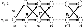
Here, Dynamic programming is employed for achieving a dual outcome, for each and every individual unit as depicted in fig1, showing the only two possible states for unit i (i.e.
U
i,t
0
or
1
). AtU
i,t
0
state, the value of the function to the minimized is unimportant (i.e., it equals zero), at the state whereU
i,t
1
, the mitigated function is
F
i
P
it
tP
it
the start-up cost and the term
tP
i,max are dropped here since the minimization is with respect toP
itMin
F
i
P
it
tP
it
is mitigated to calculate dual power with the help of optimality conditionST i
STi STi STi
t=0 t=1 t=2 t=3 t=T.l t=T V = 1i
V = 0i
Figure 1. Two-state dynamic programming
t
0
i t t i i t i
P
P
F
dP
d
(12)
The solution to this equation is
tt i
dual t i i
dS
S
dF
,
(13)
The dual power is obtained
i i t dual t i
C
b
S
2
,
(14)
Three cases to check
P
it,opt against its limits A. IfS
it,dual
S
,
then
S
it
S
imin B. IfS
imin
S
it,dual
S
imaxThen
S
it
S
it,dual
S
imin C. IfS
it,dual
P
imaxThenS
it
S
iMaxDynamic programming is employed to decide the optimal schedule of each unit over the scheduled horizon. More specifically, for each state in each hour, the on/off decision making is needed to select the lowest cost among them by conducting standard evaluation of the start-up cost and accumulated costs. The dual power calculated will be substituted in the new On/Off decision criterion.
ti t t i t t i t t
i t i t i
i
S
ST
V
S
S
S
F
,1
,1
,max (15)i = 1... NP To mitigate the above term in equation (15) at every individual hour, If
F
iS
it
ST
i,t1
V
i,t1
tS
it
tS
it
tS
it,max
0
This unit will be committed, if it does not violate the minimum downtime constraint
U
i,t
1
.4. PROPOSED MODIFIED PARTICLE SWARM OPTIMIZATION FOR LARGE SCALE UC PROBLEM
This ability of PSO to obtain optimal outcomes in n-dimensional search space with a good response rate, makes PSO stand unique globally.
PSO concentrates on timely modifying velocities of particles so that they march towards their respective
P
best andL
best values upon each time step. Whereas random numbers are fed as inputs for necessary acceleration towards attainingP
best andbest
)
(
)
(
2 21 1
1 k
i best k
i besti k
i k k
i
w
v
c
rand
P
s
c
rand
G
s
v
(16)And
s
ik1
s
ik
v
ik1 (17)In large scale problems due to its fast response characteristics, some particles tend to fly away from their vicinities which indeed causes stress on the optimizer in deciding either to bring back the particle or to neglect them. This entire process eventually contributes to increase in the calculation time to a large extent. So, this serious limitation of PSO for large scale system is surpassed by modifying the optimizer, by making it optimize initially, in a regular hypercube before it attains a feasible point. Then in our search space an optimal function “F” is assigned to quickly identify the target optimal value. For illustration, consider a “r” factored model in which we want to find out t- point optimal value.
Let
m
t
*
(
r
1
)
and let
[
0
,
1
]
mdenote the m-dimensional hypercube. Define the m*1 vector,,
)
,
,
.
.
.
,
(
~
1
s
s
tf
where xi is a r*1 vector in[
0
,
1
]
r,
i
1
,
.
.
.
,
t
,
f
[
0
,
1
]
tand define}.
0
.
1
0
.
1
|
)
,
,
.
.
.
,
(
~
{
\
s
1
s
tf
t
f
or
rs
i
for
some
i
to transform
~
into a proper model
we definethe function
F
:
(
S
r1)
t*
S
t1by
f
f
s
s
s
s
F
t t r
t
r
1
.
,
.
1
,
.
.
.
,
.
1
)
~
(
1 1
(18)The function F is invariant in the sense that
F
F
(
~
)
F
(
~
)
and the model
is based on~
s
i
s
i
/(
1
r.
s
i),
i
1
,
.
.
.
,
t
and the components in~
f
f
/(
1
k.
f
)
are their corresponding weights. The notation
F
(
~
)
signifies that the design
is transformed from
~
via the function F.Now our modified PSO algorithm is dependent on the optimal function F in Eq (18) which is employed as:
Firstly, we take a random population of “n” with “t” design points from
. For differentiating the modification, we introduce two new notations i.e. let
~
ipbest be the best position of ith particle as ofP
best. Then let
~
gbest be the global best i.e. best value of all particles among the total population as ofG
bestpreviously. The procedure of (k+1)th iteration is illustrated as follows: Generate a new velocity
v
ik1to reach to next position given by: )~ ~ ( )
~ ~
( 2 2
1 1
1 k
i pbest i k
i gbest i k
i k k
i wv crand crand
v (19)
Where
v
ik was the velocity used to get to the (k)th iteration, is the inertia weight, c1 and c2 are two pre-specific positive constants, and rand1, rand2 are m*1 uniform random vectors. The next location for the ith particle is
1 1
~
~
ki k i k
i
v
(20)If
~
ik1is not in
, we project
~
ik1to a location closest to the boundary of
. Project
~
ik1onto the regular r-simplex using i.e.
ik1
P
(
~
ik1)
and evaluate
(
ik1)
. Update the current best for each particle
~
ipbest. In this similar fashion, we find the
~
gbest after all particles are updates and continue the procedure.The entire procedure is put to an end after completion of certain user defined numbers of iterations. Finally, we obtain the required
gbest for large scale systems.5. PROPOSED MODIFIED DIFFERENTIAL EVOLUTION FOR LARGE SCALE UC PROBLEM
According to Price [13, 14], the primary pros of DE include fast application and modification, simple and easy to implement, effective global optimization capability, parallel processing nature, self-referential mutation operation, ability to handle non differentiable, noisy, and/or time-dependent objective functions etc.
are chosen randomly. Then the fitness of the new vector is checked. If the fitness of the new vector is better than the previous two, then exchange takes place.
ImplementationofDE
The implementation of DE can be illustrated in the following four steps:
5.1 Initialization –
In this step, initialization of population vector of size
N
p in random in the D-dimensional search space over a generation G as follows:min min
max
)
(
*
j j j ijrand
x
x
x
x
(21)Where i = 1, 2,
N
pdenotes the individual’s population index and j = 1, 2, D signifies the D-dimensional search space position.rand
is a uniformly distributed random number varies between 0 to 1. The upper bound and lower bound of the decision parameter are symbolized byx
minj andx
maxj respectively.Now based on obtained fitness value either of the two cases are carried out, case a: deceleration factor is indulged if fitness is not up to the mark a (or) case b: acceleration factor is indulged if fitness is better than existing ones. These inputs are fed into mutation.
5.2 Mutation –
A mutant vector, for each target vector
x
iG is formed as:)
(
*
:
/
)
(
*
:
/
) ( ) ( )
1 (
) ( ) ( )
( ) 1 (
G m G l best
G i
G m G l G
k G i
x
x
F
x
V
Best
DE
x
x
F
x
V
rand
DE
(22)
Where k, l, and m are randomly chosen vectors {1, 2….}. Further k, l and m should be different so that N > 4 is required. The mutation factor F is an experimentally chosen parameter that is used to regulate the amplification of the difference between two individuals to escape search stagnation. A special modification to this mutation factor is discussed explicitly in upcoming theory.
5.3 Crossover –
After mutation, crossover is applied to the population. For each mutant vector, a trial vector is generated as follows:
otherwise
x
j
j
or
C
rand
if
v
u
U
G ij
rand r
j G
ij G ij G i
,
)
1
,
0
(
,
(23)
Where
C
ris a crossover probability and it is fixed parameter used to create trial vectors at all generations,j
randa newly generated random value for each i.5.4 Selection –
The selection procedure compares the trial vector
U
iGand target vectorx
iGjof current position and the vector with the better fitness are allowed to enter the next generation.otherwise
x
x
f
U
f
if
U
x
G ij
G ij G
i G
i G ij
,
)
(
)
(
,
1
(24)
In case of unsatisfied termination, this process is repeated again from mutation until there is a satisfactory outcome from the operation.
But in some cases, especially for large scale problems, due to swift response abilities, DE may tend to drop regional optimums. We introduce a dynamic mutation factor in the solution algorithm for surpassing this limitation.
b
d
r
s
F
*
(
0
,
1
)
2*
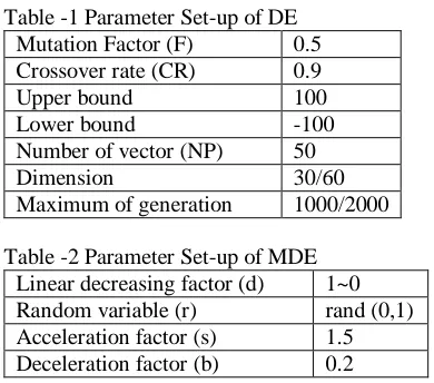
Table -1 Parameter Set-up of DE Mutation Factor (F) 0.5 Crossover rate (CR) 0.9
Upper bound 100
Lower bound -100
Number of vector (NP) 50
Dimension 30/60
Maximum of generation 1000/2000
Table -2 Parameter Set-up of MDE Linear decreasing factor (d) 1~0 Random variable (r) rand (0,1) Acceleration factor (s) 1.5 Deceleration factor (b) 0.2
6. RESULTS AND DISCUSSION
The test system containing ten power generating units and a time horizon of 24hours is taken from [9]. In PSO the population consists of 100 individuals where as in DE also the population is of 100 individuals. In lambda iteration, the tolerance is assigned to 0.0001. The fitness values of each and every individual are calculated by adding the fuel cost, the start-up cost and the penalty value. For every hour based on whether the start-up is cold start or a hot start, the appropriate cost is added to the total cost. Depending upon generation unit status, lambda iteration is used for their cost calculations. Under violation of user defined constraints such as spinning reserve requirement, tup and tdown constraints etc. we employ the necessary penalty term. All parameter values are calculated using the best settings formed as a result of a series of 10 runs. The fitness function is given below:
{[ ( ) (1 )] } }
2 lim 2
lim 1
2 lim ,
1 , ,1 u U u d D d
T
t it s p p N
i i i it it
T T K T T K S S K V V ST S F
f (26)
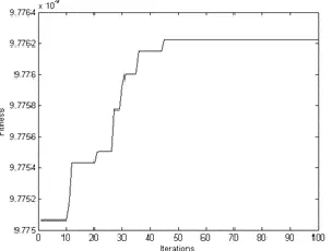
The results are depicted in Table -3, Table -4 and Table -5. The cost variations and fitness variation are depicted in Figure 2 and Figure 3 respectively for 150 iterations. The CPU run time for the following test system run is approximately 128 sec.
Table -3 Unit commitment schedule of 100 generator system (Large-scale) Hour Units On/Off Schedule
1 2 3 4 5 6 7 8 9 10 11 12 13 14 15 16 17 18 19 20 21 22 23 24
Table -4 Simulation outputs of the suggested DE method (Large-scale)
Table -5 Comparison of various methods
Figure 2. Convergence of total cost of 100-unit system with DE algorithm (Large-scale)
Figure 3. Convergence of fitness of 100-unit system with DE algorithm (Large-scale)
7. CONCLUSIONS
The first suggested method exhibits good performance in solving the unit commitment problem when it is enclosed in a hypercube before attaining a non-feasible point for a large scale problem. In parallel to this, we solved the model with DE by adding a suitable dynamic mutation factor, for obtaining the optimal settings of Lagrangian multipliers. The method has been tested for hundred units with 24 hours’ time horizon inclusive of constraints. Moreover, the test results of the suggested methods are verified with the various pre-existing methods. Hence, it could be concluded that the approach gives optimal commitment schedule of units in large scale for any given demand that satisfies the defined constraints as well as the demand with minimum cost.
No. of
Units
Best cost ($)
Average cost ($)
Worst cost ($)
10 564,180 565,922 570,509
20 1,123,321 1,124,283 1,129,199
40 2,244,193 2,250,522 2,254,122
60 3,366,628 3,372,331 3,378,352
80 4,489,722 4,492,634 4,505,124
100 5,610,001 5,621,821 5,630,851
No of
generators
Total cost ($)
LR[9] GA[9] EP[9]
PSO(Large-scale)
DE(Large-scale)
10 565,825 565,825 564,551 564,030 564,180
20 1,130,660 1,126,243 1,125,494 1,123,325 1,123,321
40 2,258,503 2,251,911 2,249,093 2,244,267 2,244,193
60 3,394,066 3,376,625 3,371,611 3,366,720 3,366,628
80 4,526,022 4,504,933 4,498,479 4,489,800 4,489,722
7. REFERENCES
[1] A. J. Wood and B. F. Wollenberg, Power Generation, Operation &Control, 2nd Ed. New York: Wiley, 1996.
[2] Yang Ting fang, T. O. Ting, “Methodological Priority List for Unit Commitment Problem”, IEEE computer society, pp.176-179, 2008.
[3] Prateek Kumar Singhal and R. Naresh Sharma, “Dynamic Programming Approach for Solving Power Generating Unit Commitment Problem”, ICCCT, pp.298-303, 2011.
[4] Arthur I. Cohen, Miki Yoshimura, “A Branch and Bound Algorithm for Unit Commitment”, IEEE Trans. Power Syst., Vol.2, pp.444-451, February 1983.
[5] Fulin Zhuang and F.D. Galiana, “Towards a more rigorous and practical unit commitment by Lagrangian relaxation”, Vol. 3, No. 2, pp.763-771, May. 1988.
[6] D. P. Kadam, P. M. Sonwane, V. P. Dhote, B. E. Kushare, “Fuzzy Logic Algorithm for Unit Commitment Problem”, International conference on control, automation, communication and energy conservation, pp1-4,2009.
[7] Musoke H. Sendaula, Saroj K Biswas, Ahmed Eltom and Cliff Parten Wilsonkazibwe, “Application of Artificial Neural Networks to Unit Commitment”, IEEE Trans. Power Syst., pp.256-260, 1991.
[8] S. A. Kazarlis, A. G. Bakirtzis and V. Petridis, “A genetic algorithm solution to the unit commitment problem”, IEEE Trans. Power Syst., vol. 11, pp. 83–92, Feb. 1996.
[9] Dimitris, N. Simopoulos, Stavroula D. Kavatza, D. Vournas, “Unit Commitment byan Enhanced Simulated Annealing Algorithm”, PSCE, pp.193-201, 2006.
[10] C. Christober, Asir Rajan and M. R. Mohan, “An Evolutionary Programming-Based Tabu Search Method for Solving the Unit Commitment Problem”, IEEE Trans. Power Syst., pp-557-585, vol.19. Feb.2004.
[11] Balci H.H. and Valenzuela J.F. “Scheduling Electric power generators using particle swarm optimization combined with the Lagrangian relaxation method”, Int.J. App Math. Comput. Sci., 14(3), pp.411421,2004.
[12] WengKee Wong, Ray-Bing Chen, Chien-Chih Huang, Weichung Wang, “A Modified Particle Swarm Optimization Technique for Finding Opti mal Designs for Mixture Models”, DOI: 10.1371/journal.pone.0124720 June 19, 2015.
[13] M.Ramu, L. Ravi Srinivas, S. Tara Kalyani, “Unit Commitment by Lagrangian Relaxation Incorporating Differential Evolution”, Journal of Electrical Engineering: Volume 15 / 2015 - Edition: 3.