Wang_unc_0153D_15007.pdf

(1)

EMPIRICAL ANALYSIS OF SEQUENTIAL TRADE MODELS FOR MARKET MICROSTRUCTURE

Tao Wang

A dissertation submitted to the faculty of the University of North Carolina at Chapel Hill in partial fulfillment of the requirements for the degree of Doctor of Philosophy in the

Department of Statistics and Operations Research.

Chapel Hill 2014

Approved by:

Chuanshu Ji

Amarjit Budhiraja

Vidyadhar Kulkarni

Haipeng Shen

(2)

c 2014 Tao Wang

(3)

ABSTRACT

TAO WANG: EMPIRICAL ANALYSIS OF SEQUENTIAL TRADE MODELS FOR MARKET MICROSTRUCTURE.

(Under the direction of Chuanshu Ji.)

Market microstructure concerns how different trading mechanisms affect asset price

for-mation. It generalizes the classical asset pricing theory, which only holds under frictionless

perfect market conditions. Most market microstructure models focus on two important

as-pects: (a) asymmetric information shared by different market participants (informed traders,

market makers, liquidity traders, et al.) (b) transaction costs reflected in bid-ask spreads.

The complexity of those models presents significant challenges to empirical studies in such

a research area. In this work, we consider some extensions of the seminal sequential trade

model in Glosten and Milgrom (Journal of Financial Economics, 1985) and perform Bayesian

MCMC inference based on the TAQ (trade and quote) database in Wharton Research Data

Services. Issues in both (a) and (b) are addressed in our study. In particular, the latent process

of fundamental asset value is modeled with GARCH volatilities; the observed and predicted

bid-ask price sequences are related by incorporating parameters for pricing errors and for

(4)

ACKNOWLEDGMENTS

First and foremost, I would like to offer my deepest gratitude to my advisor, Professor

Chuanshu Ji. It is my fortune to have Professor Ji as my academic advisor. His ingenious

thoughts and deep insight have inspired me so much and his knowledge of probability,

statis-tics and finance is a huge resource for my resarch. He is always on my back and supports me

whenever needed. Besides research, he is also a personal advisor. He cares about my career

and always gives me advice, from which I will benefit for the rest of my life, whenever I have

difficulties. In a word, I learnt so much from Professor Ji and without him, I would not have

such a wonderful experience as a Tar Heel.

I would also like to show my deep appreciation for other committee members Professor

Amarjit Budhiraja, Professor Vidyadhar G. Kulkarni, Professor Haipeng Shen and Professor

Serhan Ziya. They provide invaluable helps in my graduate study and advice for my

disser-tation. I learnt probablity and stochastic analysis from Professor Budhiraja. Professor Shen

taught me generalized linear models and functional data analysis. In addition, Professor Shen

is in Hong Kong at the time of my dissertation defense and there is a 13-hour time difference,

which is so inconvenient for him. I am extremely grateful to them. Professor Kulkarni and

Professor Ziya read my dissertation carefully and provided numerous useful comments and

feedbacks. I show many thanks to them too.

Lastly and most importantly, I would like to thank my parents as well as my older sister

and nephew. They always love, believe and support me whatever happens and sacrify a lot for

me. I hope to make them pround of me for my accomplishment. I dedicate this dissertation

(5)

TABLE OF CONTENTS

LIST OF TABLES . . . vii

LIST OF FIGURES . . . viii

1 INTRODUCTION . . . 1

2 LITERATURE REVIEW . . . 4

2.1 Roll Model . . . 4

2.2 Hasbrouck’s method . . . 6

2.3 Glosten-Milgrom Model . . . 7

2.4 Das’s approach . . . 10

2.4.1 Model . . . 10

2.4.2 Derivation of Bid and Ask Price Equations . . . 11

3 MODEL AND ESTIMATION . . . 13

3.1 Model . . . 13

3.2 Estimation . . . 15

4 SIMULATION STUDY AND MCMC . . . 17

4.1 Gibbs Sampling . . . 18

4.2 Metroplis-Hastings Sampling . . . 19

4.3 Metroplis-Hastings within Gibbs algorithm . . . 19

4.4 MCMC Convergence Diagnostics . . . 20

(6)

4.4.2 Geweke Diagnostics . . . 22

4.5 Simulation Results . . . 22

5 EMPIRICAL STUDY . . . 29

5.1 Data . . . 29

5.2 Summary Statistics of Posterior and MCMC Convergence Results . . . 32

5.3 Interpretation . . . 51

6 GARCH VOLATILITY MODEL . . . 59

6.1 Introduction to ARCH/GARCH Volatility Model . . . 59

6.2 Estimation . . . 61

6.3 Simulation Study . . . 62

6.4 Empirical Study . . . 68

6.5 Interpretation . . . 86

APPENDIX A MCMC PROCEDURE FOR THE ORIGINAL MODEL . . . 94

APPENDIX B MCMC PROCEDURE FOR THE GARCH(1,1) MODEL. . . 98

(7)

LIST OF TABLES

4.1 Summary statistics of posterior samples using simulated data. . . 23

5.1 Summary statistics of posterior samples using real BAC data. . . 33

5.2 Summary statistics of posterior samples using real MSFT data. . . 33

5.3 Summary statistics of posterior samples using real PFE data. . . 34

5.4 Summary statistics of posterior samples using real XOM data. . . 34

6.1 Summary statistics of posterior samples using simulated data (GARCH). . . . 63

6.2 Summary statistics of posterior samples using real BAC data (GARCH) . . . 68

6.3 Summary statistics of posterior samples using real MSFT data (GARCH) . . 69

6.4 Summary statistics of posterior samples using real PFE data (GARCH) . . . . 69

6.5 Summary statistics of posterior samples using real XOM data (GARCH) . . . 69

(8)

LIST OF FIGURES

4.1 Illustration of bid, ask and transction prices using simulated data . . . 24

4.2 Trace plot of posterior samples using simulated data . . . 25

4.3 Autocorrelation plot of posterior samples using simulated data . . . 26

4.4 Gelman-Rubin plot of posterior samples using simulated data. . . 27

4.5 Geweke plot of posterior samples using simulated data. . . 28

5.1 Bid and Ask prices for the real aggregation data . . . 31

5.2 Bid and Ask prices for the real aggregation data (zoomed in) . . . 31

5.3 Trace plot of posterior samples using real BAC data . . . 35

5.4 Autocorrelation plot of posterior samples using real BAC data . . . 36

5.5 Gelman-Rubin plot of posterior samples using real BAC data. . . 37

5.6 Geweke plot of posterior samples using real BAC data. . . 38

5.7 Trace plot of posterior samples using real MSFT data . . . 39

5.8 Autocorrelation plot of posterior samples using real MSFT data . . . 40

5.9 Gelman-Rubin plot of posterior samples using real MSFT data. . . 41

5.10 Geweke plot of posterior samples using real MSFT data. . . 42

5.11 Trace plot of posterior samples using real PFE data . . . 43

5.12 Autocorrelation of posterior samples using real PFE data . . . 44

5.13 Gelman-Rubin plot of posterior samples using real PFE data. . . 45

5.14 Geweke plot of posterior samples using real PFE data. . . 46

5.15 Trace plot of posterior samples using real XOM data . . . 47

5.16 Autocorrelation plot of posterior samples using real XOM data . . . 48

5.17 Gelman-Rubin plot of posterior samples using real XOM data. . . 49

5.18 Geweke plot of posterior samples using real XOM data. . . 50

(9)

5.20 The bid-ask spread VS time from the real aggregation data . . . 55

6.1 Trace plot of posterior samples using simulated data (GARCH) . . . 64

6.2 Autocorrelation of posterior samples using simulated data (GARCH) . . . 65

6.3 Gelman-Rubin plot of posterior samples using simulated data (GARCH). . . 66

6.4 Geweke plot of posterior samples using simulated data (GARCH) . . . 67

6.5 Trace plot of the posterior samples from real BAC data (GARCH) . . . 70

6.6 Autocorrelation of the posterior samples from real BAC data (GARCH) . . . 71

6.7 Gelman-Rubin plot of posterior samples using real BAC data (GARCH) . . . 72

6.8 Geweke plot of posterior samples using real BAC data (GARCH) . . . 73

6.9 Trace plot of posterior samples using real MSFT data (GARCH) . . . 74

6.10 Autocorrelation plot of posterior samples using real MSFT data (GARCH) . . 75

6.11 Gelman-Rubin plot of posterior sampels using real MSFT data (GARCH) . . 76

6.12 Geweke plot of posterior samples using real MSFT data (GARCH) . . . 77

6.13 Trace plot of posterior samples using real PFE data (GARCH) . . . 78

6.14 Autocorrelation plot of posterior samples using real PFE data (GARCH) . . . 79

6.15 Gelman-Rubin plot of posterior samples using real PFE data (GARCH) . . . 80

6.16 Geweke plot of posterior samples using real PFE data (GARCH) . . . 81

6.17 Trace plot of posterior samples using real XOM data (GARCH) . . . 82

6.18 Autocorrelation plot of posterior samples using real XOM data (GARCH) . . 83

6.19 Gelman-Rubin plot of posterior samples using real XOM data (GARCH) . . . 84

(10)

CHAPTER 1: INTRODUCTION

The research in financial economics becomes more necessary after the financial crisis,

with statistics playing an important role in such studies. Several milestones in modern

fi-nance, such as capital asset pricing model (CAPM), Black-Scholes-Merton derivatives

pric-ing, hold under certain perfect market conditions, i.e. the market is fully efficient with no

taxes, no transaction costs, no bid-ask spreads, unlimited short-selling, and all market

par-ticipants sharing the same information, to name just a few. Those assumptions are clearly

violated in real financial markets, evidenced by many empirical studies. Market

microstruc-ture concerns friction factors, aims to understand how asset price formation is affected by

various trading mechanisms.

In this work, we will focus on two aspects of market microstructure that attract most

atten-tions from financial economists: asymmetric information and bid/ask spreads. We will follow

the model-based approach in the seminal work of Glosten and Milgrom (1985), referred to

as G-M model in what follows. It is a sequential trade model assuming risk neutrality, a

quote-driven protocol. The market maker posts bid and ask prices in every (discrete) time

unit based on which traders place their orders. There are certain informed traders among

other uninformed traders in the market, and the proportion of informed traders is represented

by a parameterα. The information asymmetry induces adverse selection costs that force the

market maker to quote different prices for buying and selling, leading to the bid-ask spread.

The spread is a premium the market maker demands for trading with informed traders. A

special feature in G-M model is to present explicitly how bid and ask prices change over time

and are influenced by different trading orders.

(11)

real market data. Due to the complexity of many market microstructure models, such as G-M,

systematic model-based empirical studies are relatively lacking compared to the development

of theoretical models and model-free descriptive data analysis. A noticeable contribution is

Hasbrouck (2009) which considers an extension of Roll model [cf. Roll (1984)] and uses

the Gibbs sampler to estimate the effective trading cost and trading direction. To validate the

method, a high correlation 0.965 is calculated between the Gibbs sampler estimates of the

effective cost and the estimates based on high frequency TAQ data.

The sophisticated hierarchical and dynamic structure in G-M model presents a daunting

challenge to model-based statistical inference using real market data. Little has been done

in this direction. Das (2005) takes a useful step by presenting an algorithm for computing

approximate solutions to the bid/ask prices and runs a simulation study under the modified

G-M model. It helps us learn from the market maker’s perspective, and paves a road for

further studies.

In this work, we consider some extensions of G-M model (including Das’s) and

per-form Bayesian MCMC inference based on the TAQ (trade and quote) database in Wharton

Research Data Services. Both the asymmetric information and bid-ask spread issues are

ad-dressed. To the best of our knowledge, our work is the first attempt at inference on market

microstructure models of G-M type based on intra-day data. In the second part of our work,

we incorporate GARCH(1,1) model for the volatility of asset returns. In the first part, we

assume the volatility of equity returns is a constant over time, however, a common finding

in empirical studies of financial markets is that the variance of the returns has many stylized

facts, such as volatility clustering, leptokurtic distributions, asymmetry and leverage effect.

GARCH models are very popular under this circumstance. For that case, we present the

MCMC algorithm, and to study some properties of posterior distributions for certain

param-eters and the bid-ask spread.

(12)

afore-mentioned market microstructure models. Our model and estimation methods are presented

in Chapter 3. Chapter 4 gives a brief introduction to MCMC algorithms and conducts

simula-tion studies. Chapter 5 discusses the empirical studies, including the Wharton Research Data

Services, MCMC convergence results, the estimation results and economic interpretations.

Chapter 6 describes the GARCH(1,1) volatility model and emprical studies based on the new

model. Detailed MCMC procedures for the original and GARCH(1,1) models are provided

(13)

CHAPTER 2: LITERATURE REVIEW

There are so much work about market microstructure that we can’t present all of them.

In this Chapter, we present a partial literature review related to our work. As mentioned in

Introduction, Hasbrouck (2009) proposed a Bayesian MCMC approach based on Roll (1984)

model to estimate the effective trading cost and trading direction. As far as we know, it’s the

first work of applying Bayesian MCMC paradigm into market microstructure model. Both

the Roll (1984) model and Hasbrouck’s approach are presented here. Since G-M model is

the main framework we follow, it’s discussed following Hasbrouck’s approach. In addition,

Das (2005), by extending G-M model, develops a model of learning market maker which

explicitly compute the conditional expectation equation. He also discusses the similarities

and differences between his model and real stock market data in terms of distributional and

time series properties of returns. Das’s method can be seen as a calibration of an extended

G-M model.

2.1 Roll Model

Roll (1984) suggests a model of transaction prices which incorporates market dynamics.

This model is fundamental to many market microstructure models in the sense that it’s a

minimal structural model of security price dynamics that incorporates a bid ask spread and

it also illustrates the distinction between price movement due to fundamental security value

and those attribute to market organization and trading mechanism. Although too simple to

capture many realistic features in the market, the Roll model articulates an important aspect

of the bid-ask effect on trading price and serves as a good starting point.

(14)

For t=1,2,...,

mt=mt−1+ut, where theutare i.i.d.N(0, σ2) (2.1) wheremt is the efficient price, which means the expected terminal value of the security conditional on all public information. Theutreflect new public information. The bid and ask prices are given as

bt =mt−c

at =mt+c

(2.2)

wherecis the non-negative half-spread. And the transaction price is:

pt=mt+cqt (2.3)

wherept are the transaction price andqt are direction indicators, which take on value 1 (buy) or -1 (sell) with equal probability. The two sequences{qt} and{ut}are assumed to be independent. Note that only{pt}are observed, while{mt}and{qt}are treated as latent variables.

The model implies

∆pt=c∆qt+ut (2.4)

from which it follows

var(∆pt) = σ2+ 2c2

cov(∆pt,∆pt−1) = −c2

(2.5)

∆ptexhibits negative serial correlation as the result of effective cost. The intuition is: If

(15)

must be either 0 or−2c. And similarly, if the current price is the bid, then the price change between the next price and the current price must be either 0 or2c.

2.2 Hasbrouck’s method

The Roll model has two parameters, cand σ2_{, and also the latent variables,} _{_q

t}. Has-brouck (2009) proposed a Bayesian approach based on Roll(1984) model to estimate the

effective trading cost and trading direction. The full posterior over the parameters and latent

variables is summarized by the posterior joint distribution function f(c, σ2_{, q}_|_p₎_{, however,} it’s not in the closed form. We could get full conditional posterior distributionf(c|σ2, q, p),

f(σ2|c, q, p), and f(q|c, σ2, p)via multivariate Bayesian methods. This motivates the Gibbs sampling, which constructs full posterior densities by iteratively simulating from full

condi-tional distributions forc,σ2 _and_q_.

The model estimated by Hasbrouck’s approach genralized on the basic Roll model. The

new model is:

∆pt=c∆qt+βmrmt+ut (2.6)

wherermtis the market return on date t. It’s assumed that the market return is independent of∆qt. The sampling procedure is as follows:

• Step 0. Initialize{σ2_{, q}

1, q2,· · · , qT}, then the iterative steps are:

• Step 1. Based on the most recently simulatedσ2 and the the setqt, compute the poste-rior for the regression coefficients(candβm) and make a new draw.

• Step 2. Givenc, βm, and the setqt, compute the impliedut, make a new draw from the updated posterior forσ2_.

(16)

The trading cost estimated from US stocks are taken from 1926 to 2006 CRSP daily

data. It is also estimated by averaging all the trading costs during this period based on high

frequency trade and quote(TAQ) data. The CRSP/Gibbs estimates are very close to TAQ

estimates (with correlation 0.96), which shows that the daily Gibbs estimates have strong

validity.

Most Market Microstructure models including Roll (1984) model are dynamic over time

and have latent variables. Dynamic latent variable models can be formulated in state-space

form and estimated by maximum likelihood. However, the Bayesian paradigm and MCMC

methods make it more convenient and easy to interpret.

From statistical point, Hasbrouck’s empirical study on Roll (1984) model using MCMC

sheds light on Bayesian type of analysis on market microstructure model. However,

Has-brouck’s method has two limitations. One is that the high frequency data are not directly

used to do empirical inference. He estimates the trading cost by CRSP daily data and

com-pare the results with the estimations from the model free method using TAQ data. The other

one is that he uses the correlation between his model estimation and the model free estimation

to measure the goodness of fit, which is not so convincing.

2.3 Glosten-Milgrom Model

The model we presented here is a simplified version of the original Glosen-Milgrom

(1985) model. We follow the framwork in O’hara (1995) . Consider one security valued at

V ∈ {Vh, Vl}, withP(V =Vh) =p. The value is revealed at the end of the trade. There are three types of market participants: market makers, the informed tradersIand the uninformed

tradersU, the proportion of the informed traders isα. The market maker posts bid and ask

quotes, B and A. A trader is randomly selected from the crowd each time and submit an

(17)

market maker doesn’t know the type of the trader. He will set the bid and ask prices such that

A1 =E[V|Buy1] =VhP(Vh|Buy1) +VlP(Vl|Buy1) (2.7)

B1 =E[V|Sell1] =VhP(Vh|Sell1) +VlP(Vl|Sell1) (2.8)

and by Bayesian Formula,

P(Vh|Buy1) =

P(Buy₁|Vh)P(Vh)

P(Buy₁|Vh)P(Vh) +P(Buy1|Vl)P(Vl)

(2.9)

P(Vh|Sell1) =

P(Sell1|Vh)P(Vh)

P(Sell1|Vh)P(Vh) +P(Sell1|Vl)P(Vl) (2.10) further more,

P(Buy₁|Vh) =α+ 1

2(1−α) = 1 +α

2 ,q (2.11)

P(Buy₁|Vl) = 1−α

2 = 1−q (2.12)

P(Sell1|Vh) = 1−α

2 = 1−q (2.13)

P(Sell1|Vl) =α+ 1−α

2 =q (2.14)

so

P(Vh|Buy1) =

1+α 2 p 1+α

2 p+ 1−α

2 (1−p)

= qp

qp+ (1−q)(1−p)

(18)

and

P(Vl|Buy1) =

(1−q)(1−p)

qp+ (1−q)(1−p) (2.16)

P(Vh|Sell1) = (1−q)p

(1−q)p+q(1−p) (2.17)

P(Vl|Sell1) =

q(1−p)

(1−q)p+q(1−p) (2.18)

Next, we consider a sequence of transactions, let b denote the number of buys and s

denote the number of sells, then similarly by Bayesian formula, we can get

P(Vh|b, s) =

qb₍₁₋_q₎s_p

qb₍₁₋_q₎s_p_{+ (1}₋_q₎b_qs₍₁₋_p₎

P(Vl|b, s) =

(1−q)b_qs₍₁₋_p₎

qb₍₁₋_q₎s_p_{+ (1}₋_q₎b_qs₍₁₋_p₎

(2.19)

It can be shown that given the equations above, the bid and ask prices will converge to

the true fundamental value of the security.

One important economic justification of G-M model is trades update prices, which means

a learning process for the market maker. When the order is a buy order, since the market

maker doesn’t know which type of trader the order is from, in order to protect himself, he will

adjust his belief about the value of the stock by making an upward revision in the conditional

probability of a high outcome. Similar thing happens when it’s a sell order. As the market

maker receives trades, therefore, his expectation of the asset’s values changes, and this, in

turn, causes the bid and ask prices to change.

Another justification is that asymmetric information induces a bid-ask spread. The

asym-metric information in G-M model is the proportion of the informed traders in the population.

Asαincreases, the bid-ask spread will also increase. We will see this later in our simulation

(19)

In a word, G-M model lays foundation for the information based sequential trade model.

The limitation of G-M model is that the informed traders are drawn randomly by the

market mechanism. When he is selected, he will trade once at one unit of order but doesn’t

have any trading strategies to maximize his profit. In addition, the assumption that the true

value of the stock has two values is far from realistic.

2.4 Das’s approach

2.4.1 Model

The model is the following:

We assume that there’s only one stock trading in the market. The market maker sets bid

and ask prices at timet(BtandAtrespectively) at which he is willing to buy or sell one unit of the stock.

The stock has a true underlying valueVtat time periodt. At time periodt, a single trader is selected from the crowd and allowed to place either a (market) buy or (market) sell order

for one unit of the stock. There are two types of traders in the market, uninformed traders and

informed traders. An uninformed trader will place a buy or sell order for one unit with equal

probability, or no order with some probability if selected to trade. An informed trader who is

selected to trade knowsVtand will place a buy order ifVt > At, a sell order ifVt < Bt. The true underlying value of the stock can be considered a jump process, which means

that at time t, with probability p, a normal jump compared to the true value at t−1, with mean0, varianceσ2 _{occurs, namely,}_V

t =

  

 

Vt−1 +N(0, σ2) with probability p

Vt−1 with probability 1−p .

The market-maker attempts to track the true value over time by maintaining a probability

distribution over possible true values and updating the distribution when it receives signals

from the orders that traders place. The market maker will set the bid and ask prices so that

(20)

2.4.2 Derivation of Bid and Ask Price Equations

Letα be the proportion of informed traders in the trading crowd, and letη be the

prob-ability that an uninformed trader places a buy (or sell) order. Then the probprob-ability that an

uninformed trader places no order is1−2η.

To explicitly compute those conditional expectations, we discretize the X-axis into

inter-vals and apply Bayes’ formula, we get

E[V|Sell] = Vmax

X

Vi=Vmin

ViP(V =Vi|Sell)

= Vmax

X

Vi=Vmin

ViP(Sell|V =Vi)P(V =Vi)

P(Sell)

(2.20)

where,

P(Sell) = Vmax

X

Vi=Vmin

P(Sell|V =Vi)P(V =Vi)

= Vmax

X

Vi=Vmin

[P(Sell|V =Vi,Informed)P(Informed)

+P(Sell|V =Vi,Uninformed)P(Uninformed)]P(V =Vi) =

B−1

X

Vi=Vmin

[(α+ (1−α)η)P(V =Vi)]

+ Vmax

X

Vi=B

[((1−α)η)P(V =Vi)]

(21)

and so the bid price at time periodtis given by:

B =E[V|Sell] =

Vmax X

Vi=Vmin

P(Sell

= B−1

X

Vi=Vmin

P(Sell)

+ Vmax

X

Vi=B

P(Sell)

(2.22)

Similarly as in (2.21), we could get:

B = 1

P(Sell)

B−1

X

Vi=Vmin

((1−α)η+α)ViP(V =Vi) + Vmax

X

Vi=B

((1−α)η)ViP(V =Vi)

!

(2.23)

where,P(Sell)is given by (2.21) , and the ask price is given by:

A = 1

P(Buy) A

X

Vi=Vmin

((1−α)η)ViP(V =Vi) + Vmax

X

Vi=A+1

((1−α)η+α)ViP(V =Vi)

!

(2.24)

whereP(Buy)is given by:

P(Buy) = A

X

Vi=Vmin

[((1−α)η)P(V =Vi)] + Vmax

X

Vi=A+1

[((1−α)η+α)P(V =Vi)] (2.25)

Based on this model, Das used simulation to test the algorithm and compare the time

series and distributional properties of simulated returns with those calculated from real data.

Das’s approach sheds light on how to solve the conditional expectation equations in G-M

model. However, from the statistics point of view, no empirical analysis has been done in

(22)

CHAPTER 3: MODEL AND ESTIMATION

Our main contribution is to estimate the parameters in an extended G-M model under

Bayesian MCMC paradigm based on high frequency trade and quote(TAQ) data. In the

following three chapters, we will present our model, estimation methods, simulation results

and empirical study results.

3.1 Model

From now on, the prices we consider are all log prices. We still consider one stock in the

market. The market maker sets bid and ask prices at timet(BtandAtrespectively) at which he is willing to buy or sell one unit of the stock.

Similar to Das(2005), the stock has a true underlying valueVt at time periodt. At each timet, a single trader is selected from the crowd and allowed to place either a (market) buy

or (market) sell order for one unit of the stock. There are two types of traders in the market,

uninformed traders and informed traders. An uninformed trader will place a buy or sell order

for one unit with equal probability, or no order with some probability if selected to trade. An

informed trader who is selected to trade knows Vt and will place a buy order ifVt > At, a sell order ifVt< Bt.

The true underlying value of the stock at timetcan be considered a random walk, which

means that at timet, a normal jump, with mean0, varianceσ2 occurs, namely,Vt = Vt−1 +

N(0, σ2₎_.

Each time, the market maker sets the bid and ask price first, then the traders put their

orders. To sequentially update his belief about the true value, the market maker will set bid

(23)

a sell order on timet, andAt=Et[V|Buy], the expectation ofVtconditional on a buy order on timet.

Letαbe the proportion of informed traders in the trading crowd, andηbe the probability

that an uninformed trader places a buy (or sell) order. Then the probability that an uninformed

trader places no order is1−2η.

To explicitly compute those conditional expectations, apply Bayes’ formula, we can get

Et[V|Sell] =

Z

vpt(v|Sell)dv =

Z

vPt(Sell|v)ft(v) Pt(Sell)

dv

(3.1)

whereft(v)is the normal density ofVtandPt(Sell)is the probability of a sell order att.

Pt(Sell) = Pt(Sell|Informed)P(Informed) +Pt(Sell|Uninformed)P(Uninformed) =α

Z Bt

−∞

ft(v)dv+ (1−α)η

(3.2)

Therefore the bid price at time periodtis given by:

Bt=Et[V|Sell]

= 1

Pt(Sell)

Z ∞

−∞

vPt(Sell|v)ft(v)dv

= 1

Pt(Sell)

Z Bt

−∞

(α+ (1−α)η)vft(v)dv+

Z ∞

Bt

(1−α)ηvft(v)dv

= 1

Pt(Sell)

α

Z Bt

−∞

vft(v)dv+ (1−α)ηV0

(3.3)

Similarly, for the ask price, we have

At= 1

Pt(Buy)

α

Z ∞

At

vft(v)dv+ (1−α)ηV0

(24)

where,Pt(Buy)is given by:

Pt(Buy) = α

Z ∞

At

ft(v)dv+ (1−α)η (3.5)

3.2 Estimation

In the model, we are interested in the following parametersα: the proportion of informed

traders; η: the buying or selling probability of uninformed traders at each time period; σ2: the volatility of the jump of the underlying asset.

To estimate those parameters, since the true underlying value of the stock is a latent

vari-able, which means we can’t observe it directly, the usual estimation methods, like LSE, MLE,

don’t work here. Bayesian framework implemented with MCMC methods is applied here

since it has several advantages, both methodological and computational. Bayesian framework

offers more flexibility in modelling hierarchical data with structural changes, and are often

more easily interpretable. MCMC methods generate a discrete-time Markov chain whose

stationary distribution is the joint posterior distribution of model parameters and latent

vari-ables, hence samples from the posterior distribution of any marginal are easy to obtain by

selecting elements from the joint series.

Under Bayesian paradigm, we need to specify priors and calculate the posterior through

the likelihood.

Priors

Concerning about priors, forα, since the proportion of informed traders in the crowd

is relatively small and it’s between 0 and 1, a Beta prior with mode close to 0.l is

assigned toα. Forη, it’s also a probability parameter and no prior information about it

is available, and also there’s a constraint2η <1, so we just use a Unif(0,0.5)prior for

(25)

will stick to that one. So the priors are as follows:

α∼Beta(αα, βα)

η∼Unif(0,0.5)

σ2 ∼Unif(u1σ, u2σ)

Likelihood

In order to make the connection between the theoretical calculated bid, ask prices and

the real data, we assume that the real bid pricePb

t ∼N(Bt, δ2), and the real ask price

Pa

t ∼N(At, δ2), whereδis a small perturbation volatility term and the prior forδ2 is

δ2 ∼ Unif(u1δ, u2δ). Under these conditions, we can derive the posterior conditional distribution, which will be used in MCMC sampling.

Posterior

Our goal is to simulate samples from the joint posterior distribution. However, due

to the complexity of the model, the hierarchical structure and high dimensionality of

parameters, the joint posterior distribution is not in closed form, we can’t generate

samples directly. Therefore, MCMC is applied here. Basically, MCMC methods

gen-erate a discrete-time Markov chain whose stationary distribution is the joint posterior

distribution of model parameters and latent variables.

The following chapter gives a brief introduction to MCMC approach and the detailed

posterior distribution and MCMC procedure for our specific model are specified in

(26)

CHAPTER 4: SIMULATION STUDY AND MCMC

Under Bayesian paradigm, two types of methods are used to get samples from the

poste-rior distributions. If the density has a familiar functional form, such as a member of

exponen-tial families, a conjugate prior is chosen for the parameter, then the posterior distribution is

usually expressed in terms of conjugate probability distributions. In this case, we don’t need

numerical integration to calculate the posterior distribution due to the conjugate priors.

How-ever, the easy calculations of the posterior density comes with a price with the restrictions

imposed on the form of the prior.

A second type of computation strategy is called simulation-based methods. In many

situations, it’s unlikely that the conjugate prior is an adequate representation of the prior

state of knowledge, or the distribution density doesn’t have any conjugate priors, so that

the posterior distribution is not a familiar functional form. In such cases, the numerical

approximation or Monte Carlo simulation methods are needed.

In terms of simulation-based methods, rejection sampling with a suitable choice of

pro-posal density is a general method for simulating from an arbitrary distribution. Importance

sampling is an alternative strategy for calculating integrals and simulating from a general

posterior distribution.

Monte Carlo integration and posterior approximation via rejection sampling or

impor-tance sampling involve direct simulation from a sampling distribution, usually treated as an

approximation to the desired densityf(x). However, when the dimension of the model

be-comes large, both rejection and importance sampling will be difficult to implement as they

require the construction of a suitable proposal density which are hard to require in high

(27)

generate samples in high-dimensional problems. The idea of MCMC sampling was first

introduced by Metroplis, Rosenbluth, Teller (1953) and was subsequently generalized by

Hastings (1970). A general and detailed statistical theory of MCMC methods can be found

in Tierney (1994).

The MCMC sampling strategy relies on the construction of a Markov chain with

realiza-tionsx(0)_{, ..., x}(i)_{, ...}_{. Under appropriate regularity conditions (see Tierney (1994)),} asymp-totic results guarantee that asigoes to infinity,x(i)_{converges in distribution to}_f₍_x₎_.

In what follows, we introduce two of the most frequently used Markov Chain Monte Carlo

methods, Gibbs sampling and Metroplis-Hastings sampling, then present a combination of

the two – Metroplis-Hastings within Gibbs algorithm which is used in our Bayesian MCMC

model.

In the following algorithms, our goal is to generate samples from a density functionf(x).

While in the Bayesian paradigm,f(x)becomes the joint posterior distribution of the

param-eterθ,f(θ|data).

4.1 Gibbs Sampling

The Gibbs sampling is an algorithm based on successful generations from the full

condi-tional densities. A basic exploration can be found in Casella and George (1992). We want

to sample fromf(x1, x2, ..., xm)and assume that the full conditional density {f(xi|xj, j 6=

i), i= 1, ..., m}are available for sampling. Then the Gibbs algorithm works as follows:

1. Set the initial valuex(0) = (x(0)₁ , ..., x(0)m )0

2. Generate a new value x(n) _from _x(n−1) _{through successive generation values:} _x(n) 1 ∼

f(x1|x (n−1)

6

=1 )x (n)

2 ∼f(x2|x (n) 1 , x

(n−1) 3 , ..., x

(n−1)

m )...x(n)m ∼f(xm|x (n)

6

=m)

(28)

As the number of iterations increases, the chain approaches its stationary distribution and

convergence holds approximately.

The Gibbs sampling is the most frequently used MCMC algorithm when it’s easy to write

down the full conditional densities from which we could easily draw samples. When there

are no closed form for the full conditional densities, we might consider rejection sampling or

Metroplis-Hastings algorithm, described in the next section.

4.2 Metroplis-Hastings Sampling

Like Gibbs sampling algorithm, the Metroplis-Hastings algorithm is an iterative MCMC

method. The originator of the algorithm is Metropliset al(1953) and Hastings (1970)

intro-duced this algorithm for statistical problems. We want to generate samples from the density

functionf(x). As in rejection or importance sampling, a proposal densityq(x)from which

we can easily generate samples is required. The Metroplis-Hastings algorithm works as

fol-lows.

1. Set the initial valuex(0)

2. Generate sampley∼q(y|x(n)₎

3. x(n+1) ₌_{ y with probabilityρ(x (n)_{, y}₎

x(n) _{with probability}₁₋_ρ₍_x(n)_{, y}₎

whereρ(x, y) =min{1,f(y)q(x_f(x)q(y|_|_x)y)}

4. Repeat step 2 and 3 until enough samples are generated.

4.3 Metroplis-Hastings within Gibbs algorithm

Metropolis-Hastings(MH) within Gibbs was proposed as a hybrid algorithm that

com-bines Metropolis-Hastings and Gibbs sampling, and was suggested in Tierney (1994). In

the manner of Gibbs, one block of parameters is sampled conditional on the rest. However,

(29)

used to generate the draws. Then conditional distributions are obtained by using the fact that

when the data and a block of parameters are held fixed, the conditional density of the

remain-ing parameters is proportional to the likelihood times the prior. Then proposal densities must

be obtained by the specific problem.

For example, suppose there are 4 parameters (x1, x2, x3, x4), an MH within Gibbs may proceed with the following sequence of updates.

1. Update(x(n+1)₁ |x₂(n), x(n)₃ , x(n)₄ )using Gibbs.

2. Update(x(n+1)₂ , x(n+1)₃ |x(n+1)₁ , x(n)₄ )via Metroplis-Hastings. 3. Update(x(n+1)₄ |x₁(n+1), x(n+1)₂ , x(n+1)₃ )with Gibbs step.

Under Bayesian MCMC paradigm, we want to simulate samples from the joint posterior

distribution. In our model, there are four parameters and also a latent variable, the true

underlying value{Vt}of the asset. Using Gibbs sampling, in order to get samples from the joint posterior distribution, we can sample from the full conditional posterior distribution.

The full conditional posterior distribution is proportional to the product of the prior and the

likelihood for the corresponding parameter. If the prior is conjugate, it’s easy to simulate a

sample from the conditional posterior distribution. However, if the prior is not conjugate and

the full conditional posterior distribution is hard to sample from, we implement a

Metroplis-Hastings(M-H) within Gibbs sampling.

Please see Appendix I for the detailed M-H within Gibbs algorithm for our specific

situ-ation.

4.4 MCMC Convergence Diagnostics

A critical issue for users of MCMC methods in applications is how to determine when it

is safe to stop sampling and use the samples to estimate characteristics of the distribution of

(30)

4.4.1 Gelman-Rubin Diagnostics

Gelman and Rubin (1992) proposed a convergence diagnostic based onm(m >1)

paral-lel chains, each started from different initial values which are over-dispersed with respect to

the true distribution. Their method is based on a comparison of the within and between chain

variances for each variable. The procedure is as follows:

For each parameter:

1. Runmparallel chains of length2nwith over-dispersed starting value.

2. Disregard the firstnsamples in each chain.

3. Compute the within-chain and between-chain variance.

4. Compute the estimated variance as a weighted mean of within-chain and

between-chain variance.

5. Calculate the shrink factor.

The within-chain variance is given by W = Pm

j=1s2j

m , where s 2 j =

Pn

i=1(xij−x¯j)

n−1 is the sample variance forjth chain andx¯j =

Pn i=1xij

n . The between-chain variance is given by

B = _mn₋₁Pm

j=1(¯xj −x¯¯)

2_{, where} _x_¯_¯ ₌ Pm

j=1x¯j

m . B can be viewed as the variance of chain means multiplied by n. Then the estimated variance isV arˆ (x) = (1− 1

n)W + 1

nB and the shrink factor isRˆ =

q

ˆ V ar(x)

W . Values substantially above 1 indicate lack of convergence. A potential problem with Gelman-Rubin diagnostic is that it may mis-diagnose

conver-gence if the shrink factor happens to be close to 1 by chance. By calculating the shrink factor

at several points in time, gelman.plot in R package CODA shows if the shrink factor has

(31)

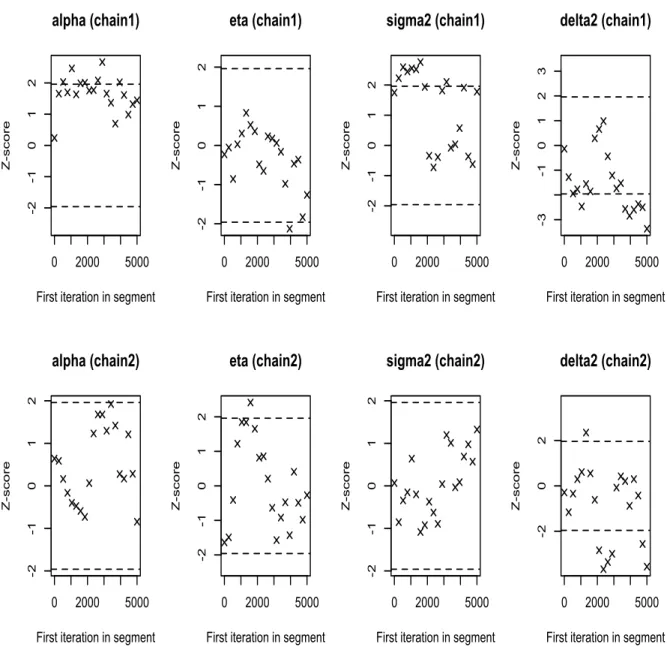
4.4.2 Geweke Diagnostics

Geweke (1992) proposed a convergence diagnostic for Markov chains based on a test for

equality of the means of the first and last part of a Markov chain (by default the first 10% and

the last 50%). If the samples are drawn from the stationary distribution of the chain, the two

means are equal and Geweke’s statistic has an asymptotically standard normal distribution.

The test statistic is a standard Z-score: the difference between the two sample means

divided by its estimated standard error. The standard error is estimated from the spectral

density at zero and so takes into account any autocorrelation. Hence values of Z which fall

in the extreme tails of a standard normal distribution suggest that the chain was not fully

converged.

If Geweke diagnostic indicates that the first and last part of a sample from a Markov chain

are not drawn from the same distribution, it may be useful to discard the first few iterations to

see if the rest of the chain has ”converged”. The geweke.plot in R package CODA shows what

happens to Geweke’s Z-score when successively larger numbers of iterations are discarded

from the beginning of the chain. To preserve the asymptotic conditions required for Geweke’s

diagnostic, the plot never discards more than half the chain.

The first half of the Markov chain is divided into several segments, then Geweke’s

Z-score is repeatedly calculated. The first Z-Z-score is calculated with all iterations in the chain,

the second after discarding the first segment, the third after discarding the first two segments,

and so on. The last Z-score is calculated using only the samples in the second half of the

chain.

4.5 Simulation Results

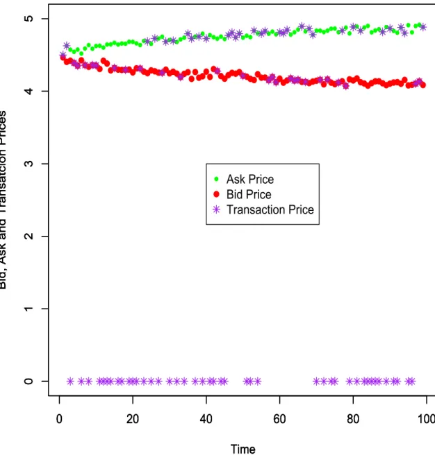
In order to test if our MCMC algorithms work well, we do simulation study first. Figure

4.1 gives us an illustration of how the bid,ask and transaction prices change over time.

(32)

the market model in Section 3.1, we calculated the Bid and Ask prices, and then use these data

to estimate the four parameters in the model by our MCMC algorithms. We run two MCMC

chains, each containing 120,000 samples, and use 20,000 burn in sample.(After the burn in

sample, we use every 10 sample as a new sample) Table 4.1 examines the effectiveness of the

estimation strategy, showing the true value, posterior summary statistics of those parameters.

We could use the posterior mean or posterior median as an estimation of the parameter.

Parameter True Value Min Median Mean Max Standard Error

α 0.2000 0.0030 0.1600 0.2300 0.5100 0.0020

η 0.2500 0.0000 0.2300 0.2500 0.5000 0.0010

σ2 0.0250 0.0021 0.0280 0.0300 0.0450 0.0000

δ2 _0.0100 _0.0000 _0.0100 _0.0100 _0.0200 _0.0000

Table 4.1: Summary statistics of posterior samples using simulated data.

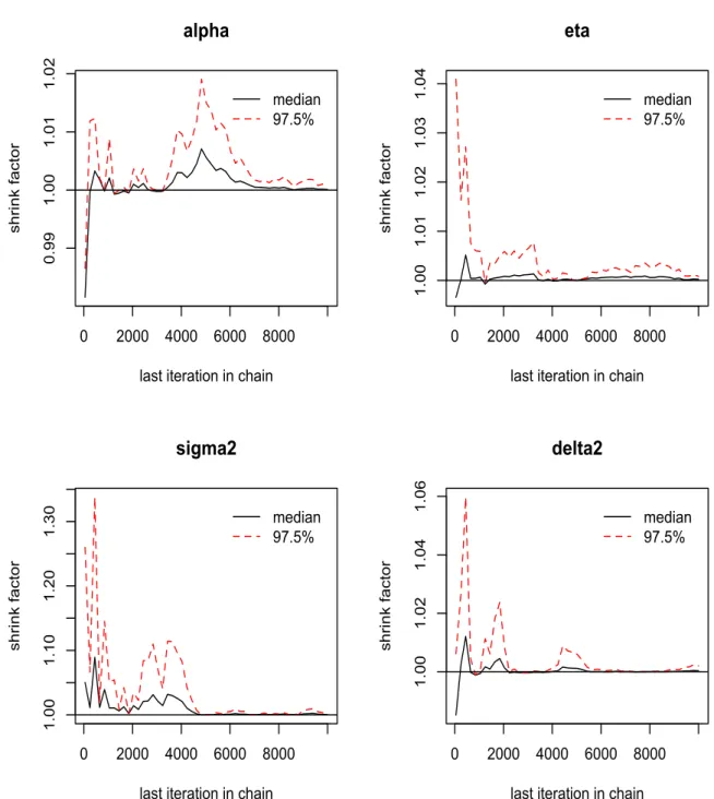
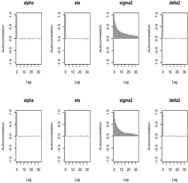
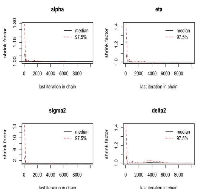
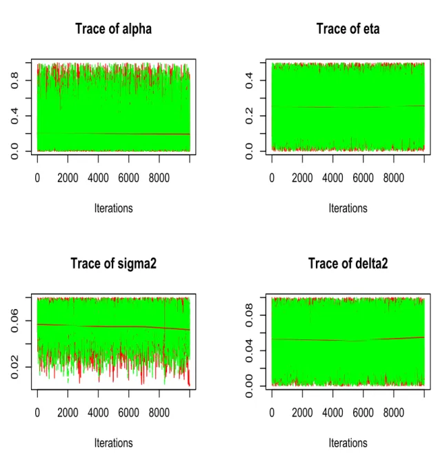
Figures 4.2-4.5 show the related convergence results of the MCMC algorithm.

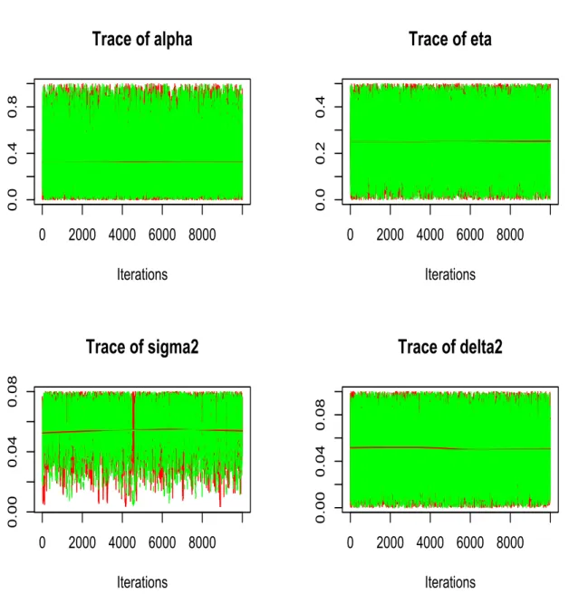
Trace plots give us a direct insight of what values the posterior samples take at each

iteration.

The autocorrelation plots show us how the autocorrelation changes with the increase of

lag. From the autocorrelation plot, we can see exceptδ2, the autocorrelations for the other 3 parameters are almost 0 at any lag. Forσ2_{, the autocorrelation decreases to 0, as the lag} increases.

From Gelman-Rubin plot, we can see that the shrink factors for all four parameters

con-verge to 1 after some iterations. Also, from Geweke plot, most of the Z-scores for all

pa-rameters are between -1.96 and 1.96. Both the Gelman-Rubin and Geweke plot show good

MCMC convergence.

Seeing the similarities between the posterior estimation and the true value of the

pa-rameters and MCMC convergence, we can conclude that our MCMC algorithm works well.

(33)

0 20 40 60 80 100

0

1

2

3

4

5

Time

Bi

d

,

Ask

a

n

d

T

ra

n

sa

tci

o

n

Pri

ce

s

0 20 40 60 80 100

0

1

2

3

4

5

Time

Bi

d

,

Ask

a

n

d

T

ra

n

sa

tci

o

n

Pri

ce

s

0 20 40 60 80 100

0

1

2

3

4

5

Time

Bi

d

,

Ask

a

n

d

T

ra

n

sa

tci

o

n

Pri

ce

s

Ask Price Bid Price

Transaction Price

(34)

0 2000 4000 6000 8000

0.0

0.2

0.4

0.6

0.8

1.0

Iterations Trace of alpha

0 2000 4000 6000 8000

0.0

0.1

0.2

0.3

0.4

0.5

Iterations

Trace of eta

0 2000 4000 6000 8000

0.01

0.02

0.03

0.04

Iterations

Trace of sigma2

0 2000 4000 6000 8000

0.000

0.010

0.020

Iterations

Trace of delta2

(35)

0 10 20 30 -1 .0 -0 .5 0.0 0.5 1.0 Lag Au to co rre la tio n alpha

0 10 20 30

-1 .0 -0 .5 0.0 0.5 1.0 Lag Au to co rre la tio n eta

0 10 20 30

-1 .0 -0 .5 0.0 0.5 1.0 Lag Au to co rre la tio n sigma2

0 10 20 30

-1 .0 -0 .5 0.0 0.5 1.0 Lag Au to co rre la tio n delta2

0 10 20 30

-1 .0 -0 .5 0.0 0.5 1.0 Lag Au to co rre la tio n alpha

0 10 20 30

(36)

0 2000 4000 6000 8000

0.99

1.00

1.01

1.02

last iteration in chain

sh

ri

n

k

fa

ct

o

r

median 97.5% alpha

0 2000 4000 6000 8000

1.00

1.01

1.02

1.03

1.04

sh

ri

n

k

fa

ct

o

r

median 97.5% eta

0 2000 4000 6000 8000

1.00

1.10

1.20

1.30

sh

ri

n

k

fa

ct

o

r

median

97.5%

sigma2

0 2000 4000 6000 8000

1.00

1.02

1.04

1.06

sh

ri

n

k

fa

ct

o

r

median 97.5% delta2

(37)

0 2000 4000 -2 -1 0 1 2

First iteration in segment

Z

-sco

re

alpha (chain1)

0 2000 4000

-2

-1

0

1

2

Z

-sco

re

eta (chain1)

0 2000 4000

-2

-1

0

1

2

Z

-sco

re

sigma2 (chain1)

0 2000 4000

-2

-1

0

1

2

Z

-sco

re

delta2 (chain1)

0 2000 4000

-2

-1

0

1

2

Z

-sco

re

alpha (chain2)

0 2000 4000

-2

-1

0

1

2

Z

-sco

re

eta (chain2)

0 2000 4000

-2

-1

0

1

2

Z

-sco

re

sigma2 (chain2)

0 2000 4000

-2

-1

0

1

2

Z

-sco

re

delta2 (chain2)

(38)

CHAPTER 5: EMPIRICAL STUDY

5.1 Data

The data we used are the bid and ask prices of Microsoft stock on April and May, 2013

from trade and quote (TAQ) database. The Trade and Quote (TAQ) database contains intraday

transactions data (trades and quotes) for all securities listed on the New York Stock Exchange

(NYSE) and American Stock Exchange (AMEX), as well as Nasdaq National Market System

(NMS) and SmallCap issues. We consider four different equties from four different sectors:

Bank of America Corporation (Ticker: BAC), Microsoft Corporation (Ticker: MSFT), Pfizer

Inc. (Ticker: PFE), Exxon Mobile Corporation (Ticker: XOM). We divide the data into

training set and test set. The April data is the training set and the May data is the test set.

Since the data are recorded tick by tick, it’s high frequency and has tons of observations

for one month. For example,the microsoft data in April 2013 has around 28,000,000

obser-vations in total, each day has over 900,000 obserobser-vations and so there are about 13 tradings

at each time spot during each trading day.There are perhaps two major problems if we do

empirical study using the raw bid and ask prices. One is the computational burden. Since the

time horizon we can handle is at most several hundreds considering the computation time,

under the raw data style, the sample size we could use is relatively small. The other one is that

there’s too much noise in the original high frequency data. So in order to do our empirical

study, some data manipulation techniques are applied here.

• Firstly, the missing data are deleted.

(39)

• Thirdly, since trading are heavier at the beginning and the end of the trading day, while thinner at lunch time, we participated each day into 5 periods: 9:30 to 10:00, 10:00 to

11:30, 11:30 to 2:30, 2:30 to 3:30, 3:30 to 4:00 and used the mean of the bid and ask

price during each period.

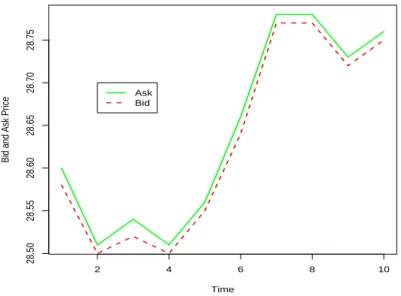
Figure 5.1 shows the bid and ask prices for the cleaned data. From Figure 5.1, it’s hard to

see the difference between the bid and ask prices since the difference is usually 1 or 2 cents,

extremely small compared to the bid and ask prices. So in order to see the difference, we

(40)

0 20 40 60 80 100

29

30

31

32

33

Time

Bid and Ask Pr

ice

Ask Bid

Figure 5.1: Bid and Ask prices for the real aggregation data

2 4 6 8 10

28.50

28.55

28.60

28.65

28.70

28.75

Time

Bid and Ask Pr

ice

Ask Bid

(41)

5.2 Summary Statistics of Posterior and MCMC Convergence Results

Tables 5.1 to 5.4 show the summary statistics of the posterior samples for all the four

parameters of different equities. Again, we could use posterior mean or posterior median to

estimate those parameters. From Table 5.1 to 5.4, we can see that the posterior estimations of

αandσ2_{vary from equities to equities, while the estimations of}_η_and_δ2_{are almost the same} for all four equities. Sinceηis the probablity of a buy or sell order of an uninformed trader,

it doesn’t change among different equities, so isδ2_{, the pertubation between the theoretical} and real bid and ask prices. While the proportion of informed traders and the volatility of

returns depend on equities.

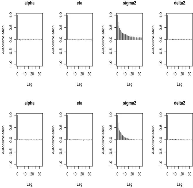
Figures 5.3-5.18 show the convergence results of the MCMC algorithms for all four

eq-uities. Similar to the analysis in the simulation study, we could conclude that the MCMC

algorithms converge. However, although the autocorrelation ofσ2_{decreases as lag increases,} it still exists. This suggests us that the constant volatility model may not be an appropriate

(42)

Parameter Min Median Mean Max Standard Error

α 0.0000 0.2871 0.3500 0.9998 0.0019

η 0.0000 0.2502 0.2502 0.5000 0.0010

σ2 0.0028 0.0564 0.0533 0.0800 0.0001

δ2 _0.0000 _0.0504 _0.0503 _0.1000 _0.0002

Table 5.1: Summary statistics of posterior samples using real BAC data.

α 0.0000 0.1646 0.2495 1.0000 0.0017

η 0.0000 0.2509 0.2512 0.5000 0.0010

σ2 _0.0036 _0.0573 _0.0544 _0.0800 _0.0001

δ2 _0.0000 _0.0526 _0.0518 _0.1000 _0.0002

(43)

α 0.0000 0.2905 0.3533 1.0000 0.0019

η 0.0000 0.2513 0.2507 0.5000 0.0010

σ2 0.0030 0.0358 0.0337 0.0500 0.0000

δ2 _0.0000 _0.0513 _0.0508 _0.0100 _0.0002

Table 5.3: Summary statistics of posterior samples using real PFE data.

α 0.0000 0.1644 0.2476 0.9993 0.0017

η 0.0000 0.2517 0.2512 0.5000 0.0010

σ2 _0.0024 _0.0353 _0.0336 _0.0499 _0.0000

δ2 _0.0000 _0.0522 _0.0516 _0.1000 _0.0002

(44)

0 2000 4000 6000 8000

0.0

0.4

0.8

Iterations

Trace of alpha

0 2000 4000 6000 8000

0.0

0.2

0.4

Iterations

Trace of eta

0 2000 4000 6000 8000

0.00

0.04

0.08

Iterations

Trace of sigma2

0 2000 4000 6000 8000

0.00

0.04

0.08

Iterations

Trace of delta2

(45)

0 10 20 30 -1 .0 -0 .5 0.0 0.5 1.0 Lag Au to co rre la ti o n alpha

0 10 20 30

-1 .0 -0 .5 0.0 0.5 1.0 Lag Au to co rre la ti o n eta

0 10 20 30

-1 .0 -0 .5 0.0 0.5 1.0 Lag Au to co rre la ti o n sigma2

0 10 20 30

-1 .0 -0 .5 0.0 0.5 1.0 Lag Au to co rre la ti o n delta2

0 10 20 30

-1 .0 -0 .5 0.0 0.5 1.0 Lag Au to co rre la ti o n alpha

0 10 20 30

(46)

0 2000 4000 6000 8000

1.00

1.15

1.30

sh

ri

n

k

fa

ct

o

r _median

97.5%

alpha

0 2000 4000 6000 8000

1.0

1.2

1.4

sh

ri

n

k

fa

ct

o

r _median

97.5%

eta

0 2000 4000 6000 8000

2

6

10

14

sh

ri

n

k

fa

ct

o

r _median

97.5%

sigma2

0 2000 4000 6000 8000

1.0

1.2

1.4

sh

ri

n

k

fa

ct

o

r _median

97.5%

delta2

(47)

0 2000 5000 -2 -1 0 1 2

Z

-sco

re

alpha (chain1)

0 2000 5000

-2

-1

0

1

2

Z

-sco

re

eta (chain1)

0 2000 5000

-2

-1

0

1

2

Z

-sco

re

sigma2 (chain1)

0 2000 5000

-6 -4 -2 0 2 4 6

Z

-sco

re

delta2 (chain1)

0 2000 5000

-2

-1

0

1

2

Z

-sco

re

alpha (chain2)

0 2000 5000

-3 -2 -1 0 1 2 3

Z

-sco

re

eta (chain2)

0 2000 5000

-2

-1

0

1

2

Z

-sco

re

sigma2 (chain2)

0 2000 5000

-2

-1

0

1

2

Z

-sco

re

delta2 (chain2)

(48)

0 2000 4000 6000 8000

0.0

0.4

0.8

Iterations

Trace of alpha

0 2000 4000 6000 8000

0.0

0.2

0.4

Iterations

Trace of eta

0 2000 4000 6000 8000

0.02

0.06

Iterations

Trace of sigma2

0 2000 4000 6000 8000

0.00

0.04

0.08

Iterations

Trace of delta2

(49)

0 10 20 30 -1 .0 -0 .5 0.0 0.5 1.0 Lag Au to co rre la ti o n alpha

0 10 20 30

-1 .0 -0 .5 0.0 0.5 1.0 Lag Au to co rre la ti o n alpha

0 10 20 30

(50)

0 2000 4000 6000 8000

1.00

1.10

1.20

sh

ri

n

k

fa

ct

o

r _median

97.5%

alpha

0 2000 4000 6000 8000

1.00

1.02

1.04

sh

ri

n

k

fa

ct

o

r _median

97.5%

eta

0 2000 4000 6000 8000

1.0

1.4

sh

ri

n

k

fa

ct

o

r _median

97.5%

sigma2

0 2000 4000 6000 8000

1.00

1.04

1.08

sh

ri

n

k

fa

ct

o

r _median

97.5%

delta2

(51)

0 2000 5000 -2 -1 0 1 2

Z

-sco

re

alpha (chain1)

0 2000 5000

-2

-1

0

1

2

Z

-sco

re

eta (chain1)

0 2000 5000

-2

-1

0

1

2

Z

-sco

re

sigma2 (chain1)

0 2000 5000

-3 -1 0 1 2 3

Z

-sco

re

delta2 (chain1)

0 2000 5000

-2

-1

0

1

2

Z

-sco

re

alpha (chain2)

0 2000 5000

-2

-1

0

1

2

Z

-sco

re

eta (chain2)

0 2000 5000

-2

-1

0

1

2

Z

-sco

re

sigma2 (chain2)

0 2000 5000

-2

0

2

Z

-sco

re

delta2 (chain2)

(52)

0 2000 4000 6000 8000

0.0

0.2

0.4

0.6

0.8

1.0

Iterations

Trace of alpha

0 2000 4000 6000 8000

0.0

0.1

0.2

0.3

0.4

0.5

Iterations

Trace of eta

0 2000 4000 6000 8000

0.01

0.02

0.03

0.04

0.05

Iterations Trace of sigma2

0 2000 4000 6000 8000

0.00

0.04

0.08

Iterations Trace of delta2

(53)

0 10 20 30

(54)

0 2000 4000 6000 8000

0.98

1.00

1.02

1.04

sh

rin

k

fa

ct

or

0 2000 4000 6000 8000

1.00

1.01

1.02

1.03

sh

rin

k

fa

ct

or

median 97.5% eta

0 2000 4000 6000 8000

1.00

1.10

1.20

1.30

sh

rin

k

fa

ct

or

median 97.5% sigma2

0 2000 4000 6000 8000

1.0

1.2

1.4

1.6

sh

rin

k

fa

ct

or

median 97.5% delta2

(55)

0 2000 4000 -2 -1 0 1 2

Z

-sco

re

alpha (chain1)

0 2000 4000

-2

-1

0

1

2

Z

-sco

re

eta (chain1)

0 2000 4000

-2

-1

0

1

2

Z

-sco

re

sigma2 (chain1)

0 2000 4000

-3 -2 -1 0 1 2 3

Z

-sco

re

delta2 (chain1)

0 2000 4000

-3 -2 -1 0 1 2 3

Z

-sco

re

alpha (chain2)

0 2000 4000

-2

-1

0

1

2

Z

-sco

re

eta (chain2)

0 2000 4000

-3 -2 -1 0 1 2 3

Z

-sco

re

sigma2 (chain2)

0 2000 4000

-4

-2

0

2

4

Z

-sco

re

delta2 (chain2)

(56)

0 1000 2000 3000 4000 5000

0.0

0.2

0.4

0.6

0.8

1.0

Iterations

Trace of alpha

0 1000 2000 3000 4000 5000

0.0

0.1

0.2

0.3

0.4

0.5

Iterations Trace of eta

0 1000 2000 3000 4000 5000

0.01

0.03

0.05

Iterations Trace of sigma2

0 1000 2000 3000 4000 5000

0.00

0.04

0.08

Iterations Trace of delta2

(57)

0 10 20 30

(58)

0 1000 2000 3000 4000 5000

1.00

1.02

1.04

1.06

sh

rin

k

fa

ct

or

0 1000 2000 3000 4000 5000

0.98

1.02

1.06

1.10

sh

rin

k

fa

ct

or

median

97.5%

eta

0 1000 2000 3000 4000 5000

1.0

1.1

1.2

1.3

sh

rin

k

fa

ct

or

median 97.5%

sigma2

0 1000 2000 3000 4000 5000

0.99

1.01

1.03

1.05

sh

rin

k

fa

ct

or

median 97.5%

delta2

(59)

0 1000 2000 -2 -1 0 1 2

Z

-sco

re

alpha (chain1)

0 1000 2000

-2

-1

0

1

2

Z

-sco

re

eta (chain1)

0 1000 2000

-2

-1

0

1

2

Z

-sco

re

sigma2 (chain1)

0 1000 2000

-3 -2 -1 0 1 2 3

Z

-sco

re

delta2 (chain1)

0 1000 2000

-2

-1

0

1

2

Z

-sco

re

alpha (chain2)

0 1000 2000

-2

-1

0

1

2

Z

-sco

re

eta (chain2)

0 1000 2000

-3 -2 -1 0 1 2 3

Z

-sco

re

sigma2 (chain2)

0 1000 2000

-2

-1

0

1

2

Z

-sco

re

delta2 (chain2)

(60)

5.3 Interpretation

Glosten-Milgrom model captures the notion of asymmetric information, explicitly

char-acterizing the bid-ask spread. The bid-ask spread is the difference between the price at

which liquidity suppliers are willing to buy(ask) and the price at which they are willing to

sell(bid).In the market microstructure theoretical models, there are three sources of bid-ask

spread: First, the adverse selection costs arising with asymmetric information. Second, the

inventory costs, those the market maker must sustain for holding undesired positions. The

third one is the order processing cost, which is associated with the handling of a transaction.

In G-M model, the bid-ask spread is due to the first one. The assumption of asymmetric

information generates adverse selection costs, which oblige market makers to quote different

prices for buying and selling, i.e. to open the bid-ask spread. The spread is the premium that

market makers demand for trading with agents with superior information. The asymmetric

information in G-M model is reflected by α, the proportion of the informed traders in the

crowd. Since asymmetric information determines the bid-ask spread, we could imagine that

the bigger α is, the more informed traders, the larger the bid-ask spread will be. Figure

5.19 shows us how the value of α affects the bid-ask spread in the simulation study. The

conclusion is that with the increase ofα, the bid-ask spread also increases. Proposition 5.3

provides us a theoretical justification of our conclusion.

In order to showAt−Btis an increasing function ofα, we can show that the derivative of

At−Btaboutαis positive for sufficiently smallα. We consider approximating the bid-ask spreadAt−Btas a linear function ofαfor sufficiently smallα >0, i.e. at everyt, we want to write

At−Bt=a0+a1α+o(α) (5.1)