Displays for exploration and comparison of nested or intersecting surfaces

(1)

Displays for Exploration and Comparison of Nested or Intersecting

Surfaces

by

Christopher Charles Weigle

A dissertation submitted to the faculty of the University of North Carolina at Chapel Hill in partial fulfillment of the requirements for the degree of Doctor of Philosophy in the Depart-ment of Computer Science.

Chapel Hill 2006

Approved by:

Russell M. Taylor II, Advisor

Elizabeth Bullitt, Reader

Christopher G. Healey, Reader

Stephen M. Pizer, Reader

(2)

c

2006

(3)

ABSTRACT

CHRISTOPHER CHARLES WEIGLE: Displays for Exploration and Comparison of Nested or Intersecting Surfaces.

(Under the direction of Russell M. Taylor II.)

The surfaces of real-world objects almost never intersect, so the human visual system is ill

pre-pared to deal with this rare case. However, the comparison of two similar models or approximations of

the same surface can require simultaneous estimation of individual global shape, estimation of point

or feature correspondences, and local comparisons of shape and distance between the two surfaces. A

key supposition of this work is that these relationships between intersecting surfaces, especially the

local relationships, are best understood when the surfaces are displayed such that they do intersect.

For instance, the relationships between radiation iso-dose levels and healthy and tumorous tissue is

best studied in context with all intersections clearly shown.

This dissertation presents new visualization techniques for general layered surfaces, and

inter-secting surfaces in particular, designed for scientists with problems that require such display. The

techniques are enabled by a union/intersection refactoring of intersecting surfaces that converts them

into nested surfaces, which are more easily treated for visualization. The techniques are aimed at

exploratory visualization, where accurate performance of a variety of tasks is desirable, not just the

best technique for one particular task. User studies, utilizing tasks selected based on interviews with

scientists, are used to evaluate the effectiveness of the new techniques, and to compare them to some

existing, common techniques. The studies show that participants performed the user study tasks more

(4)

ACKNOWLEDGMENTS

I thank my advisor, Russell Taylor, and my committee members, Elizabeth Bullitt, Christopher

Healey, Steven Pizer, and Mary Whitton, for their advice and guidance in this work.

I thank the scientists, Elizabeth Bullitt, Ed Chaney, Micheal Falvo, and Amitabh Varshney, for

discussing their research with me and for helping determine the direction of this work.

I thank the faculty and staff of the computer science department for their many years of support

and for providing all the little things that make up an excellent learning environment.

I thank the National Science Foundation and the National Institutes of Health for financial support.

I thank family and friends who supported and encouraged me throughout my at Carolina. Most

(5)

LIST OF TABLES

2.1 Domain-specific questions . . . 12

2.2 Generic questions . . . 14

5.1 List of user study experiments . . . 77

A.1 Participant responses from User Study 1.1 . . . 135

(10)

LIST OF FIGURES

2.1 Tumors segmented from MRI Data . . . 7

2.2 Example 3D radiation treatment planning image . . . 9

2.3 Example AFM scan of a cilium . . . 10

2.4 Example molecular docking interfaces . . . 11

3.1 Kinetic depth effect . . . 24

3.2 Color mapping for distance . . . 29

3.3 Asymmetry in Euclidean shortest distance between surfaces . . . 30

3.4 Ambiguity in Euclidean shortest distance between surfaces . . . 30

3.5 Wireframe visualization . . . 31

3.6 Grid visualization . . . 32

3.7 Ribbon visualization . . . 32

3.8 Cutaway visualization . . . 33

3.9 View-dependent transparency visualization . . . 34

3.10 Regularized texture visualization . . . 34

3.11 Principal curvature texture visualization . . . 35

3.12 Complex texture visualization . . . 36

3.13 Uncertainty visualizations . . . 37

3.14 Uncertainty visualizations . . . 38

3.15 Probabilistic visualizations . . . 38

4.1 Rendering refactored surfaces . . . 43

4.2 Union-intersection refactoring . . . 44

4.3 Red-Blue color mapping technique . . . 46

4.4 Red-Green color mapping technique . . . 47

4.5 Point-correspondence technique . . . 49

(11)

4.7 Principal curvature texture with cast shadows technique . . . 52

4.8 Principal curvature texture with point-correspondence glyphs technique . . . 54

4.9 Comparing principal texture to isotropic texture . . . 55

4.10 Overlay illustration technique . . . 56

4.11 “The Veiled Maiden” . . . 56

4.12 Retriangulating an intersected triangle . . . 62

5.1 Example bump data . . . 83

5.2 Example user study trial . . . 84

5.3 Color mapping example . . . 86

5.4 Principal curvature example . . . 87

5.5 Cast shadows example . . . 89

5.6 User Study 1.1 results . . . 92

5.9 Global shape task data . . . 103

5.10 Color mapping examples . . . 105

5.11 Principal curvature texture examples . . . 106

5.12 Cast shadows examples . . . 107

5.13 Point-correspondence examples . . . 108

5.14 Texture and correspondence examples . . . 110

5.15 Ishihara color blindness test . . . 111

(12)

Chapter 1 Introduction

The ultimate goal for layered-surface visualization is to simultaneously present nested or

inter-secting surfaces such that the shape of each is just as understandable as if it were displayed alone

while enabling comparisons amongst the surfaces. The surfaces of real-world objects almost never

intersect, so the human visual system is ill prepared to deal with this rare case. However, the

compari-son of two similar models or approximations of the same surface can require simultaneous estimation

of individual global shape, estimation of point or feature correspondences, and local comparisons of

shape and distance between the two surfaces. A key supposition of this work is that these

relation-ships between intersecting surfaces, especially the local relationrelation-ships, are best understood when the

surfaces are displayed such that they do intersect.

This work presents novel visualization techniques for general layered surfaces, designed for

sci-entists with problems that require such display. The techniques developed for this work are enabled

by two algorithms also presented here. The first algorithm refactors intersecting surfaces into

non-intersecting, nested surfaces. The second algorithm computes a bijective map between two surfaces,

where the map is suitable for use in visualizing integral lines of point correspondence between

sur-faces (as an aid to perceiving inter-surface distance).

The effectiveness of the two new techniques at conveying the shape of layered surfaces is evaluated

by a series of user studies. The tasks included in the user studies are distilled from interviews with

(13)

interviewed work in a range of fields, including medicine, biology, physics, and chemistry.

The user study tasks derived from these domains and domain-specific questions are the following:

• estimating and comparing inter-surface distances,

• estimating and comparing local shape, and

• recognizing global shape.

Other tasks were also identified through interviews with the scientists, such as identification of the

intersection and volume estimation and comparison, but these were not evaluated by user study for

reasons explained in Chapter 2.

1.1 Thesis Statement

The thesis of my dissertation is the following:

Union/intersection refactoring of intersecting surface geometry into non-intersecting

com-ponents enables the effective application of existing nested-surface visualization

tech-niques to general layered-surface data. Two novel layered-surface display techtech-niques,

re-lying on the refactoring algorithm and utilizing 1) cast shadows or 2) point-correspondence

glyphs, enable better shape perception for a pair of general, layered surfaces than a set

of previous techniques. The novel techniques also preserve the ability to comprehend the

global shape of the individual surfaces.

This work, only a step toward the ultimate goal for layered-surface visualization, takes the

follow-ing approach:

• collect domain-specific layered-surface questions from scientists,

• synthesize domain-independent layered-surface questions suitable for guiding the design of

(14)

• design layered-surface display techniques that present two surfaces in a manner enabling the

simultaneous perception of surface shape and the comparison of shapes and related metrics

between surfaces, and

• run evaluation studies to quantify the effectiveness of these techniques at displaying layered

surfaces in general, and the synthesized questions specifically.

1.2 Organization

Chapter 2 motivates this work by describing the scientists’ research and enumerating their major

questions involving the shapes of and relationships between layered surfaces. The scientists work in a

variety of fields, and each could benefit from displays of intersecting surfaces. The scientists questions

are generalized and categorized to show how the disparate questions relate to a small number of shape

metrics. The chapter concludes with the synthesis of performance tasks for evaluating techniques that

address the scientist’ questions.

Chapter 3 presents the relevant factors of visual perception, shape analysis, and visualization

that drive the development of effective visual display. It describes existing techniques for displaying

multiple nested surfaces and surfaces with positional uncertainty, which this work draws upon.

Chapter 4 describes five techniques, three existing and two new, included in the user study

evalu-ations. For completeness, two proposed techniques not included in the user study are also described.

The new techniques are enabled by a union/intersection refactoring of intersecting surfaces (also

de-scribed in Chapter 4) that converts intersecting surfaces into nested interior and exterior surfaces. The

first of the new, studied techniques uses shadows cast from the exterior surface onto the interior

sur-face to enhance the perception of depth and separation between the sursur-faces. The second of the new,

studied techniques instead uses point-correspondence glyphs to do the same.

Chapter 5 describes user studies designed to evaluate the effectiveness of the two techniques.

The performance tasks utilized in the user study are derived from the scientist interviews. The novel

(15)

as layered-surface visualizations.

Chapter 6 summarizes the dissertation work and the reviews the contributions made to

(16)

Chapter 2 Driving Problems

This work is particularly focused on visualization techniques that enable scientists to perform

multiple comparisons between surfaces. A common difficulty in introducing new visualization

tech-niques to a scientist’s workflow is proving the value of the new technique to the scientist’s research.

Therefore, this work undertook identification of the key questions of interest to a group of scientists

working in different domains. The questions then inform the design of user studies to indicate how

well a given visualization conveys the information in which the scientists are interested.

The following sections will explore the scientists’ expectations for layered-surface visualization

and how those expectations are transformed into user-study tasks. First, each scientist’s area of

re-search will be described and specific investigations described. Then generic questions will be

synthe-sized. Finally, measurable performance tasks suitable for user studies evaluating shape perception of

layered-surface visualization techniques will be derived from the set of questions.

The hypothesis that many domain-specific questions map to a small number of generic tasks was

shown to be reasonable; the 15 domain-specific questions from 4 domains mapped to 6 generic tasks.

The questions posed by a new scientist caused no new generic questions, suggesting that the set tested

(17)

2.1 Scientists: Domains and Investigations

This section contains background information on the scientists, their research areas, and their

investigations as they pertain to intersecting surfaces.

2.1.1 Medicine: Evaluating Tumor Image Segmentation Algorithms

Many medical image volumes are collected by computed tomography (CT) or magnetic resonance

imaging (MRI). CT image volumes represent the amount of radiation absorbed by the different tissues

in the scanned region. Tissues with different absorption properties produce different intensity levels

in the CT image volume. MRI image volumes primarily represent the resonant response of

hydro-gen atoms to radio frequency excitation. Tissues with different hydrohydro-gen content produce different

responses to the imaging signal, which translates to different intensity levels in the MRI volume.

Whatever the imaging method, structures are identified within the image volume by a process called

image segmentation.

Computer-aided image segmentation techniques distinguish groups or regions of pixels1or vox-els2 that form an object or objects separate from the background of an image [ACKT96]. Some segmentation methods require hand-selecting image elements, some are fully computer-automated,

and some lie in between. The result of the image segmentation is a labeled image representing the

object or objects of interest found in the image volume. The labeled image may then be used to

con-struct shape representations of the individual labeled regions. It is not important to this work what the

representation is, except that it can be readily converted to a boundary representation.

Dr. Elizabeth Bullitt (Department of Neurosurgery at UNC Chapel Hill) is interested in

layered-surface display for applications involving brain tumors extracted from MRI volumes. Dr. Bullitt is

especially interested in tools for comparing different segmentations of the same data (i.e. human

versus computer) and tools for assisting surgical or chemotherapy planning for tumor treatment.

1_{The word}_pixel_{comes from the phrase}_{picture element. A pixel represents a single sample of the data represented by}

a 2D image. The amount of data summarized by a single pixel depends on the details of the image capture or generation method.

(18)

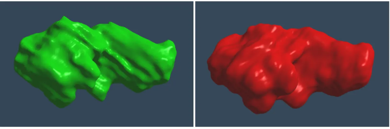
One of Dr. Bullitt’s goals is to develop image segmentation algorithms capable of segmenting

brain tumors from MRI volumes with at least the same accuracy and reliability as expert radiologists.

Such algorithms might then be trusted by clinicians to help with treatment planning. Understanding

the differences between automatic segmentations and expert segmentations can help determine how

to tune the automatic algorithms. A particular question is whether differences between two

segmen-tations are correlated to shape features (see Figure 2.1). For instance, if the automatically-extracted

tumor boundary consistently overestimates the height and width of similar small protrusions, as

com-pared to the expert-extracted tumor boundary, this may indicate that the parameters controlling the

contribution of small-scale features in the image data are too sensitive.

Figure 2.1: On the left, a tumor segmented from MRI data by hand. On the right, the same tumor segmented from the same MRI data by automatic algorithm.

2.1.2 Medicine: Tumor Radiation Treatment Planning

There are three main methods of treating tumors: chemotherapy, surgery, and radiation. Treatment

of tumors by radiation involves arranging multiple low-dose radiation beams to deliver a high dose

at their intersection. The planning of the positions, shapes, and magnitudes of the low-dose radiation

beams is very complex, and fully-automated planning remains an area of active research. Thus,

radi-ation treatment planning is still guided by human experts who must fully understand the relradi-ationships

between tumors, healthy tissue, and the radiation concentration levels.

(19)

(GTV). The GTV does not contain extensions of the tumor smaller than the resolution of the imaging

technology, nor does it contain regions of surrounding tissue experts expect to be damaged by the

presence and growth of the tumor. The extent of these extensions and regions can be predicted from

tumors with similar pathology. Thus, a radiologist defines aclinical target volumethat encompasses

the GTV and these un-imaged regions. Finally, aplanning target volume(PTV) is defined to contain

the CTV and a small margin allowing for patient motion between and during treatments.

Each low-dosage beam should deliver minimal radiation to healthy tissues while the intersection

of the beams should deliver a high level of radiation within the PTV. Typically, radiologists determine

the arrangement of beams manually with the aid of 2D planning images of the tumor and surrounding

tissues. Software tools for determining the placements and strengths of radiation sources often present

radiation iso-dose boundaries that depict treatment regions receiving up to selectable threshold of

radiation dose. The most commonly used software tools still present planning images in 2D, both to

facilitate the experience of current radiological experts and to satisfy regulations governing records

and approval of radiation treatment.

Dr. Edward Chaney (Department of Radiology/Oncology at UNC Chapel Hill) is interested in

layered-surface display for applications involving the planning of radiation treatment of tumors. His

interests include development of segmentation techniques for the tumor and organs and their

com-bined 3D display along with iso-dose surfaces (see Figure 2.2). Dr. Chaney leads research into the

development of 3D displays for radiation planning applications. He is interested in effective displays

of tumor, organs, and iso-dose surfaces enabling clinicians to choose appropriate dose levels and allow

for the typical day-to-day shifting of anatomy in a patient undergoing radiation therapy. For instance,

radiologists may be able to make better treatment plans from 3D displays that enable the surgeon to

understand the relationships between radiation iso-dose surfaces, the tumor, and surrounding healthy

(20)

Figure 2.2: An example of an image from a 3D radiation treatment planning system [LFP+90]. Such systems enable a clinician to layout the position, shape, and magnitude of multiple low-dose radiation beams to focus the beams’ intersection on the tumorous tissue. The beams’ intersection delivers a high dose of radiation to the tumor while individual beams deliver acceptably low doses to nearby healthy tissues.

2.1.3 Materials Science: Atomic-Force Microscopy

An atomic-force microscope (AFM) is capable of imaging many physical properties along the

sur-face of a microscopic specimen, such as height, conductivity, friction, and viscosity [BQG86]. AFMs

collect height images of specimens by feedback-controlled scanning of the surface of the specimen

with a probe. The tip is scanned to an image coordinate, at which point the height data is recorded.

The probe typically has a tip tens of nanometers across, enabling an AFM to image structures as

small as an individual virus or strand of DNA. The resulting height data, effectively a dilation of the

specimen by the tip, can be used directly to construct a height field for surface display.

Dr. Michael Falvo (Curriculum of Applied Materials Science at UNC Chapel Hill) is interested in

layered-surface display for comparing AFM scans of real specimens with simulated scans computed

from models of the specimen and the microscope. An AFM simulator performs geometric dilation

of a specimen model by a model tip. Understanding the differences between the real and simulated

(21)

heights are not significantly different between the two surfaces but the slopes are different, the most

likely explanation is that the tip model is the wrong shape.

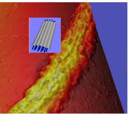
One of Dr. Falvo’s particular interests is the structure of human lung cilia (see Figure 2.3). Height

images of cilia taken by AFM show length-wise, striated ridges that may be the result of a fiber-bundle

structure within the cilia. Comparison to simulated AFM scans of modeled fiber bundles may help

determine the likely size and number of fibers in an individual cilium.

Figure 2.3: An AFM scan of a cilium specimen overlaid with a geometric model of the internal structure of cilia. Note the striations along the length of the AFM scan of the specimen; it is these features the geometric model is intended to capture.

2.1.4 Molecular Docking: Protein Interfaces

Molecular docking applications aid in understanding the minimum-energy configuration and

ge-ometric arrangement of molecules as they bond to form more complex compounds. These

applica-tions must make use of chemistry, geometry, hydrophilic properties, atomic charge, etc., between two

molecules to produce probable docking configurations. Often, these probable docking configurations

(22)

multi-ple algorithms for computing solvent-accessibility surfaces, but the general approach is to determine

contact points between a fixed probe and the computed electron density shells of all the atoms in the

interacting molecules.

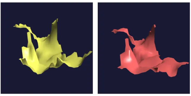
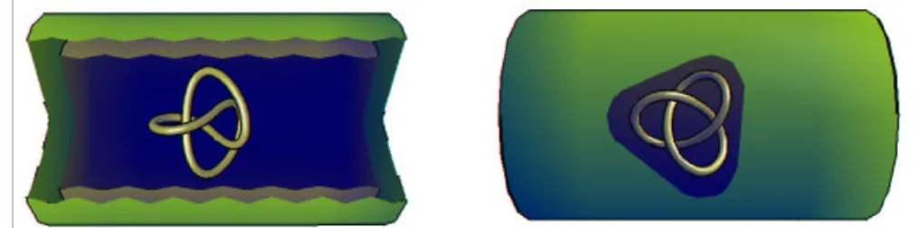
Dr. Amitabh Varshney (Department of Computer Science at the University of Maryland) is

in-terested in layered-surface display of computed protein docking configurations. Dr. Varshney has

developed many algorithms to produce probable docking geometries for pairs of molecules. More

recently, his research group has developed algorithms that produce only the interaction sites, called

interface surfaces, of the solvent-accessible surfaces for a pair of molecules (see Figure 2.4). He wants

to visually inspect the interface surfaces as a high-speed filtering step to determine if the docking

ar-rangement is probable. The filtering step should enable easy identification of arar-rangements where the

interface surfaces intersect. The filtering step should also enable easy identification of arrangements

where there is insufficient clearance between interface surfaces to allow enzymes to span the two

surfaces and form a molecular bond.

(23)

2.2 Mapping to Generic Questions

This section describes the mapping from domain-specific scientist questions to generic questions.

The aim is to show that domain-specific questions from a variety of sources can be mapped to just a

few general questions. Later, these generic questions will be used to identify the measurable

perfor-mance tasks to be tested via user studies.

I anticipate that the set of domain-specific questions from scientists in a broad spectrum of

dis-ciplines will map to a small number of generic goals for layered-surface display. In that case, it will

be possible to evaluate different techniques with respect to their ability to effectively provide answers

to this small number of goals. Then, by selecting the appropriate goal, the best technique for each

domain-specific question can be determined.

2.2.1 Mapping: Scientist Questions

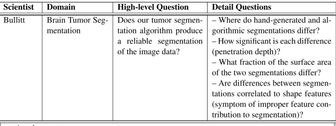
Table 2.1 presents the list of scientists, their domains of interest, and their high-level questions.

The table also shows a breakdown of the high-level questions into more specific questions, revealing

how the scientists expect to explore their data sets to answer their high-level questions.

Table 2.1: Domain-specific questions asked by scientists.

Scientist Domain High-level Question Detail Questions

Bullitt Brain Tumor Seg-mentation

Does our tumor segmen-tation algorithm produce a reliable segmentation of the image data?

– Where do hand-generated and al-gorithmic segmentations differ? – How significant is each difference (penetration depth)?

– What fraction of the surface area of the two segmentations differ? – Are differences between segmen-tations correlated to shape features (symptom of improper feature con-tribution to segmentation)?

(24)

continued from previous page

Scientist Domain High-level Question Detail Questions

Falvo Real vs. Simu-lated AFM Scans

Does the geometric model of the specimen explain the features found in the real AFM scan?

– Does one scan contain significant features not found in the other? – Does the simulated scan appear to be wider or narrower near the spec-imen substrate than the real scan (symptom of incorrect tip shape)? – Does the simulated scan appear to be higher or lower near the object peaks than the real scan (symptom of incorrect specimen shape)? – Are the shape differences consis-tent with misalignment of the two scan surfaces?

Chaney Tumor Radiation Planning

Is the planned dose level a good fit to the organs and tumor?

– Where is the dose not a good fit to the tumor (penetration depth)? – Where is the dose not a good fit to the organs (penetration depth)? Chaney Kidney

Segmen-tation

How does the shape of the segmentation vary with the weighting of two heuristics for thresholding the image?

– Where are the segmentations not a good match?

– Where the segmentations are not a good match, how much difference is there?

– Do the two segmentations have a high percentage of volume overlap?

Varshney Docked Protein Interface Surfaces

Does the interface be-tween two proteins sug-gest a probable docking configuration?

– Do the two surface intersect? – Where is there insufficient clear-ance between the two surfaces?

2.2.2 Mapping: Specific to Generic Questions

Table 2.2 presents domain-specific questions and their mapping to generic questions. The generic

questions are numbered to show overlap between domains. The fifteen domain-specific questions

from four scientists in three different domains map to eight generic questions (six questions are

num-bered, but question number 4 comes in three related forms that depend on the transformation being

hypothesized between the two surfaces). Two are very local questions (2, 6), two consist of statistics

(25)

variations or the volumes of space enclosed by the surfaces (3, 5). As described in the next section, the

summary statistics are better found through calculation than visualization. Also described is a method

for reducing the set of hypothesis questions to a single shape task.

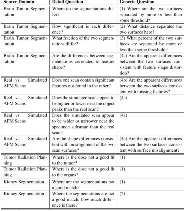
Table 2.2: Mapping of domain questions to generic questions.

Source Domain Detail Question Generic Question Brain Tumor

Segmen-tation

Where do the segmentations dif-fer?

(1) Where are the two surfaces separated by more or less than some threshold?

Brain Tumor Segmen-tation

How significant is each differ-ence?

(2) What distance separates the two surfaces here?

Brain Tumor Segmen-tation

What fraction of the two segmen-tations differ?

(3) What percent of the two sur-faces are separated by more or less than some threshold? Brain Tumor

Segmen-tation

Are the differences between seg-mentations correlated to feature shape?

(4a) Are the apparent differences between the two surfaces con-sistent with feature shape distor-tion?

Real vs. Simulated AFM Scans

Does one scan contain significant features not found in the other?

(4b) Are the apparent differences between the two surfaces consis-tent with missing features? Real vs. Simulated

AFM Scans

Does the simulated scan appear to be higher or lower near the object peaks than the real scan?

(4a)

Does the simulated scan appear to be wider or narrower near the specimen substrate than the real scan?

(4a)

Are the shape differences consis-tent with misalignment of the two scan surfaces?

(4c) Are the apparent differences between the two surfaces consis-tent with surface misalignment? Tumor Radiation

Plan-ning

Where is the dose not a good fit to the tumor?

(1)

Tumor Radiation Plan-ning

Where is the dose not a good fit to the organs?

(1)

Kidney Segmentation Where are the segmentations not a good match?

(1)

Kidney Segmentation Where the segmentations are not a good match, how much differ-ence is there?

(2)

(26)

continued from previous page

Source Domain Detail Question Generic Question

Kidney Segmentation Do the two segmentations have a high percentage of volume over-lap?

(5) What percent of the total (union) volume is contained in the overlap (intersection) vol-ume?

Docked Protein Inter-face SurInter-faces

Are the two surfaces free of inter-sections?

(6) Where are the surface inter-sections?

Docked Protein Inter-face SurInter-faces

Is there sufficient clearance be-tween the two surfaces?

(1)

2.3 Mapping: Grouping Questions Toward Tasks

This section explores the similarities between many of the generic questions. In particular, it

describes the mapping of the generic questions onto tasks appropriate for user-study evaluation of

layered-surface visualizations. In some cases it is argued that no evaluation be performed. Such cases

involve generic questions that do not map well to shape perception tasks because the human visual

system is not well suited to estimating the shape property to be explored.

Questions 1, 2, and 3 are strongly related. All three questions are concerned with estimating the

distance between the surfaces. Question 1, Where are the two surfaces separated by more or less

than some threshold?, asks to compare the distance separating two surfaces at some local region with

some reference distance. Question 2,How far apart are the two surfaces here?, asks what the actual

distance is between the surfaces given a point of reference on one surface. Question 3,What percent

of the two surfaces are separated by more or less than some threshold?, asks what fraction of the

surfaces satisfies question one. If user studies show that participants can compare separating distances

accurately with a particular two-surface visualization technique, then it is predicted that questions one

and three can be answered accurately. Question 2, however, asks for a direct measurement. This is not

a task the human visual system performs well. Our ability to visually measure distance relies on our

ability to compare apparent distances to some reference such as a ruler or other known distance. In as

much as the human visual system can estimate distance, answering question two accurately follows

(27)

Question 6,Where are the surface intersections?, is related to the distance questions (1, 2, and 3).

The intersections are the regions where the surface separation is zero. Though it could be grouped with

the distance questions, the most direct way to enable intersection questions is to explicitly compute

and display them (with an unused perceptual cue) as part of the visualization. Assuming a

percep-tually salient, direct display of the intersection can be added to any display techniques developed

in this dissertation, specifically measuring user study performance at identifying the intersection is

unnecessary.

Question 4 appears in three related parts, Are the apparent differences consistent withsome

hy-pothesis? The three hypotheses aremisalignment,missing features, andfeature distortion. All three

hypotheses are concerned with comparing the shape of the two surfaces. The misalignment

hypothe-sis tests whether the two surfaces are the same shape but were not brought into a common coordinate

system. The missing-feature hypothesis tests whether the surfaces are different shapes. The feature

distortion hypothesis tests whether corresponding features are systematically exaggerated on one

sur-face.

These domain-specific shape hypotheses require understanding of their meaning (i.e., what does

it mean for a feature to be dilated) that goes beyond low-level shape perception into cognition and are

more difficult to isolate from the problem domain. Also, there are many more possible hypotheses

than the ones solicited from this group of scientists. In this dissertation, the combination of a local

shape perception task and a broad shape perception task (such as global shape recognition) serves to

cover the visual-perception aspects of the hypothesis questions. The global shape task also serves to

show whether the visualization techniques greatly interfere with the comprehension of the individual

objects.

Question 5, What percent of the union volume is contained in the intersection volume?, asks a

completely global question. This is more than a perception question, as one must estimate volume of

two complex, composite shapes resulting from the intersection of the two principal shapes (the

union-of-two-shapes boundary and the intersection-union-of-two-shapes boundary). Unfortunately, the human

visual system is not well suited to volume estimation tasks even for single physical objects. It is

(28)

overlap statistics about their surface would be better served by computing them outright.

2.4 Tasks

This section lists the tasks proposed to cover the synthesized questions. Recall that these

ques-tions were about distance, shape, volume, or the intersection itself. Also recall that a volume task

was deemed unnecessary due to the human visual system’s poor ability to estimate volume and that

an intersection task was deemed unnecessary because it is dominated by directly displaying the

in-tersection curves via a salient perceptual cue. The following tasks appear to exercise the remaining

synthesized generic questions.

• Distance Task: Indicate in which of two regions the two surfaces are closest together. This task

addresses generic questions one, two, and three – the distance questions.

• Local Shape Task: Indicate in which of two regions the two surfaces are most nearly parallel.

This task addresses generic question four – the shape hypothesis question – at a small scale.

• Global Shape Task: Identify which, if either, of the two shapes contains a target shape. This

task addresses generic question four at a large scale. This task also shows the interference the

different visualization techniques cause for recognizing shapes.

(29)

Chapter 3 Background

As stated in the introduction, the ultimate goal for layered-surface visualization is to

simultane-ously present nested or intersecting surfaces such that the shape of each is just as understandable as

if it were displayed alone while enabling local comparison amongst the surfaces. To approach this,

it must be understood what is meant by shape, how it is perceived by the human visual system, and

what techniques have proven to best present single and multiple surfaces.

This chapter presents background and related work in geometric shape, visual perception, and

surface visualization. The first section describes the geometry of shape as it pertains to display and

comprehension of shape. The second section describes perceptual cues commonly used to display a

single surface and their relationship to geometric shape. The final section describes existing

visualiza-tion techniques for displaying multiple surfaces, organized by intended interpretavisualiza-tion of the display,

with special attention given to those leveraging perceptual cues.

3.1 Geometry of Shape

The following sections, indeed the majority of this chapter, deal with the display and visual

per-ception of object shape. This chapter begins with a discussion of what constitutes object shape. This

section will introduce terms and concepts used in describing the geometry of shape1

1_{Often, shape and depth are used to denote similar visual concepts. For instance, the manner in which visual depth,}

(30)

3.1.1 Mathematics of Shape

This section introduces many important concepts and terms used in the study of geometric shape.

The content of this section is heavily influenced by readings of Jan Koenderink’s excellent text on the

subject,Solid Shape[Koe90].

Thegeometric shapeof an object is an operational concept describing, to a linear approximation,

how the object’s surface changes within a neighborhood. The shape of the object at some point on its

surface depends not only on the object, but also on the size of the neighborhood (the scale) considered.

The first-order approximation of an object’s surface at a point is thetangent plane2of the surface at that point. The tangent plane serves as a reference frame for understanding how the surface changes

within the neighborhood of the surface point. The tangent plane is the first derivative of object shape.

On the surface, the tangent plane is a 2D reference frame. The direction orthogonal to the

tan-gent plane is called thesurface normal. The surface normal is a more computationally convenient

entity than the tangent plane and is more commonly used in computer graphics as a local

approxi-mation of shape. Together the surface normal and tangent plane define a 3D reference frame for the

neighborhood about a point on the surface of an object.

As the tangent plane is only a local linear approximation to the surface at a point, the true surface

deviates from the tangent plane as you move about the surface away from that point. Thecurvature

at that point on the surface is the measure of the rate of this deviation, and is the second derivative of

surface shape.

The shape operatorreveals how the tangent plane changes for a step within the local

neighbor-hood, so it captures the complete local curvature. Specifically, the shape operator is a matrix operator

that gives the change in the surface normal for a step along each basis vector of the tangent plane (thus

it contains partial derivatives of the surface normal with respect to the basis vector directions). The

shape operator describes a linear system, so the change in surface normal direction due to a step in an

however, the term depth will be used exclusively to denote ordering of objects, or part of objects, in the scene with respect to the observer.

2_Let₍_x

0,y0,z0)be any point on the surfacez= f(x,y). If the lines tangent to all smooth curves on the surface passing

(31)

arbitrary direction can be composed of a linear combination of steps along the basis vectors.

By solving for the eigen terms of the linear system represented by the shape operator, the

mini-mum and maximini-mum change in the surface normal for a step in the tangent plane can be determined.

The eigen vectors of the shape operator give basis vectors for the tangent plane that are also the

direc-tions of maximum and minimum change in surface normal. The associated eigen values are then the

minimum and maximum curvatures. Specifically, the maximum direction and associated curvature

are referred to as thefirst principal directionandfirst principal curvature. The minimum direction

and curvature are referred to as the second principal direction and curvature. These eigen vectors

are, of course, orthogonal. An important property of the principal directions is that they are pure

nose-dive curvatures; for a step along the direction of principal curvature, the surface normal changes

only toward or away from that same direction of principal curvature (according to the sign of the

curvature).

The determinant of the shape operator is called theGaussian curvature. The magnitude of

Gaus-sian curvature is a measure of the spread of the surface normals within a neighborhood. The sign

of the Gaussian curvature in a local area of the surface can easily be estimated just be viewing the

surface. Concave areas have a negative Gaussian curvature. Convex areas have a positive Gaussian

curvature. Flat areas have zero Gaussian curvature. The Gaussian curvature is so named because of its

relationship to theGauss mapof a surface. The Gauss map maps points on a surface, via their surface

normal, to points on a unit sphere (in this case called the Gaussian sphere). Gaussian curvature is also

a measure of the magnification of a locality when mapped to the Gaussian sphere.

The trace of the shape operator divided by two is themean curvature. The mean curvature is an

average of the change of the surface normal over all directions.

3.1.2 Geometric Shape and View Projection

Many features of surface shape have special importance for understanding the shape of a

projec-tion of an object as viewed from some vantage point. These features contribute to the depth

(32)

shadows – shadow boundaries are the projections of these same features from the light source onto

the shadow receiver.

Thefoldis the locus of all points on the surface that are tangent to the viewing direction. Though it

may be composed of several loops, the fold is always closed. For a given viewing direction, however,

parts of the fold may be occluded by the surface itself.

The occlusion boundaryof the surface is the locus of points that divide the surface into visible

and invisible regions. The occlusion boundary is that portion of the fold that is not occluded by the

surface. Though concave regions of the surface may contribute to the fold, they can never contribute

to the occlusion boundary as they would be simultaneously occluded.

Thecontouris the projection of the occlusion boundary onto an image. The contour may contain

T-junctions, cusps, and terminations. As the view direction moves, changes in the apparent shape of

the projection of the surface originate along the contour.

The external portions of the contour are called thesilhouetteof the surface. The silhouette is the

closed boundary of projection and separates the visible object from the background.

The contour conveys important global shape information about the projected shape. The sign of

the curvature of the contour indicates the local Gaussian curvature in that area, an area necessarily

orthogonal to the current view direction. Where the contour is convex, the surface is convex. Where

the contour is concave, the surface is saddle shaped. Where the contour is flat, the surface is cylindrical

or planar. Similar information can be determined from the shadow boundaries.

Geometry of Illumination

The amount of light reflected off a region of surface and reaching an observer is called the

lumi-nance. Surface shape plays a key role in determining how luminance is distributed, that is how the

light from the light source is spread out as it reflects off a surface. In the section, the total luminance

from a surface reaching a single observer will be referred to as theluminance image.

(33)

func-tions; the luminance of a Lambertian surface, which reflects incident light uniformly in all directions,

and the luminance of specularities, which are images of the light source reflected onto the observer.

The luminance of a Lambertian surface follows Lambert’s cosine law and varies in intensity

ac-cording to the cosine of the angle between the direction of incident light and the direction of the

surface normal. Features of the shape of a Lambertian surface appear as similar features of the

in-tensity of the luminance image of the surface [Koe90]. Generic regions of the surface, local shape

features that continue to exist after a random perturbation of the surface (elliptics, hyperbolics, etc.),

appear as generic regions of the luminance. Singularities of surface curvature, local shape features

that may be annihilated by a random perturbation of the surface (saddle points, cusps, etc.), appear as

singularities of the luminance.

Specularities follow the Snell’s law reflection of a point light about the surface normal and onto

the viewing direction. Given a point on a surface with unit surface normaln and a directionl to a

point light source, specularities appear in the reflection directionrwhenr=l−2(n·l)n. The Gauss

map of a surface is formed by taking the direction of all unit surface normals as the coordinates on

the unit sphere. So a single point on the surface maps to coordinates on the Gauss map through that

point’s unit normal. If a path along the surface crosses a parabolic point (a point with zero Gaussian

curvature), the corresponding path along the Gauss map will contain a fold. Pairs of specularities

are generated and annihilated at parabolic points on the surface [Koe90], so the number of folds on

the Gauss map (also called the multiplicity of the Gauss map) determines the maximum number of

specularities on the surface. Note that even non-generic shapes that contain no parabolic points (a

sphere) or only parabolic points (a plane) still display a single specularity.

3.2 Displaying a Single Surface

Much work in visual perception explores the perception of shape from shading [BB90, CK97,

CJ96, DHEN95, Gib50, Ram88]. Specifically, the human visual system interprets shape with a

built-in bias toward scenes that are diffusely lit from overhead [Gib50] - though sufficient cues from other

(34)

that also elicit the perception of shape, such as texture [CJ96], specular highlights [BB90], shadows

[EKK93], and object boundaries [Ram88].

3.2.1 Depth Cues

Monocular depth cues are important for understanding the arrangement of objects in a scene and

their relative sizes. However, only some of these depth cues appear frequently in scientific or medical

visualization. Occlusion and linear perspective are depth cues present in most 3D scientific or

med-ical visualizations. The kinetic depth effect is commonly found in visualization either through user

interaction (i.e. interactive applications) or precomputed motion (i.e. animations). Depth of field and

atmospheric attenuation are not commonly found in scientific or medical visualization.

Occlusion is an important monocular depth cue where a point near the observer obscures more

distant points. The occlusion boundaries are key elements in conveying relative depth between objects.

Occlusion is also important to the understanding of the global shape of objects, as an object’s internal

contours tell the observer both about the relative ordering of regions of the surface and about the shape

of the surface at the region forming the contour.

Perspective foreshortening is the name for the most commonly observed artifact of projecting a 3D

scene onto a 2D imaging device (a digital camera, a retina, etc.). Distant objects appear smaller than

nearby objects. The perspective projection maps 3D space such that parallel lines receding from the

imaging device are mapped into lines converging to a single vanishing point in the projected image.

Because this projection preserves straight lines, it is often referred to as linear perspective. One side

effect of perspective projection is that the apparent depth of familiar objects is related to their apparent

size. For instance, if in the same scene a child appears larger than an adult, the natural interpretation

is that the adult is much further away than the child.

Depth of field is an “out of focus” effect on unattended objects at depths different from the attended

object. Due to the lens of the eye focusing the attended object onto the fovea, other objects in the

view appear blurred. Atmospheric attenuation is an effect of diminishing contrast due to atmospheric

(35)

of field and atmospheric attenuation are not commonly included in visualization for two reasons.

First, graphics hardware has only recently been capable of producing depth-of-field and

atmospheric-attenuation effects at interactive rates. More importantly, both effects reduce overall detail in the

visualization. They are more often used to focus attention than to enhance depth relationships.

The kinetic depth effect is a strong depth cue derived from motion cues. An object near the

observer moving transverse to the line of sight at a fixed velocity traverses a greater visual angle per

unit time than does an identical object with a similar absolute motion but at a greater depth from the

observer. Figure 3.1 illustrates this phenomenon. This is similar in effect to parallax, the change in

relative apparent positions of objects produced by a change in the position of the observer.

Figure 3.1: This figure illustrates the phenomenon of thekinetic depth effect. The two objects move with the same absolute velocity relative to the observer. The difference in apparent velocity reveals their relative depths from the observer.

The kinetic depth effect also applies to the understanding of shape of a single object in motion.

The difference in appearant velocities of multiple regions of an object in motion reveal depth and

shape information about the full object.

Depth cues also result from stereo vision. Because this work does not use or evaluate stereo as

an active perceptual component of layered-surface display, it will not be discussed in detail here. It

should be noted, however, that the kinetic depth effect is a stronger shape cue than stereo vision. So for

(36)

good shape perception.

3.2.2 Direct Illumination

The most common illumination model used in computer graphics, the empirical Phong lighting

model, may convey shape cues in a manner similar to certain real objects under natural illumination.

The Phong lighting model approximates diffuse and specular lighting according to Lambert’s cosine

law and Fresnel’s laws of reflection, respectively [Pho75]. Under the appropriate conditions, Phong

illumination has been shown to convey shape and depth [JC96]. Phong’s diffuse term captures the

view-independent Lambert’s Law reflection of a point light about the surface normal. Phong’s

spec-ular term captures the Snell’s law reflection of a point light about the surface normal and onto the

viewing direction.

Johnston et al. investigated whether the illusion of curvature in Phong-illuminated,

computer-generated surfaces mimic cues appearing on solid objects under real light [JC96]. Specifically, they

looked at three-dimensional curvature contrast and the illuminant-position effect. Three-dimensional

curvature contrast is a simultaneous contrast effect for curved surfaces, in that the apparent curvature

of a surface defined by shading is influenced by the surrounding surface curvature. The

illuminant-position effect predicts that the perceived magnitude of curvature of a surface patch is a function of

the position of the light source. The illuminant-position effect can be mitigated by texture cues and

specularities. Johnstonet al. found the perceived curvature magnitudes influenced by both

investi-gated effects to be the same whether the objects were real or computer generated – the Phong lighting

model works.

The Phong illumination model is used in all of the techniques presented here.

3.2.3 Shadows

Shadows on surfaces can be categorized into two types – attached shadows and cast shadows.

Attached shadows contain points on a surface facing away from the light source. Cast shadows contain

(37)

correspond to light rays that just graze the surface producing the shadow. Generically, attached shadow

boundaries denote the curve along the surface where surface normal vectors are perpendicular to the

incoming light direction. Cast shadow boundaries are the projection of the attached shadow boundary.

Shadow formation shares similarities with specular hightlights. Shadows are created and

de-stroyed at parabolic points on the surface. Shadows also occur in pairs, just as specularities do. A

shadow pair consists of one attached and one cast shadow. Other shape-related properties of shadow

boundaries and their interaction with surface features are described in Knillet al.[KMK97].

Research into the perception of attached shadows finds that they are perceived similarly to

occlu-sion contours [EKK93, Cas01, KMK97, MKK98]. Occluocclu-sion contours separate objects from

back-ground and also reveal the global structure of surfaces, providing evidence of the presence of bumps,

dimples, and other features [Koe84].

Cavanagh and Leclerc report that cast shadows help disambiguate light direction and help place

objects in space but do not appear to strongly suggest shape [CL89]. Cavanagh and Leclerc also

find that shape perception is diminished for shadows that do not obey appropriate contrast rules –

the region in shadows should be darker than the surround. Indeed, “light” shadows, false shadows

that geometrically behave like real shadows but are brighter than their surroundings instead of darker,

appear to be processed differently from “dark” shadows in visual search tasks.

Sinha reports that viewers are not very sensitive to inconsistencies in the directions of cast shadows

for disconnected objects in doctored photographs [Sin00].

Shadows in motion produce a strong sense of 3D object motion but not illuminant motion.

Ma-massian et al. report that even when available visual information suggests otherwise, shadows in

motion are interpreted as if the light source were fixed [MK96]. Other assumptions and biases can be

overridden by shadow motion as well, such as constant object size, linear object motion, and assumed

viewpoint.

Another benefit of shadows is that they can enforce the perception of proximity or contact between

objects [TSS+98]. Physically inaccurate, artificial shadows placed near the region of closest proximity

(38)

understanding the layout of a scene.

One of the techniques presented here uses dark cast shadows from a fixed light source as a depth

cue.

3.2.4 Texture

Texture has long been known to be an excellent shape cue. Gibson showed that the slant of a

tex-tured plane extending to the horizon could be perceived, though the slant is typically underestimated

[Gib50]. Here Gibson uses slant to refer to the degree of rotation of the surface out of the image plane

and toward the horizon. Cumminget al. described the three shape cues due to apparent variation in

texture on a uniformly textured surface: compression– due to surface orientation relative to the

im-age plane,density– due to distance and obliqueness of view, andperspective– due to distance from

the view point [CJP93]. Of these, texture compression has been shown to be the most significant for

surface shape perception under stereo viewing.

A number of studies have found that certain directional components of surface texture seem to

enable better shape and depth perception than some other directions [IFP96, IFP97, KHSI03, KHSI04,

LZ00, SW04]. Li and Zaidi find that (sinusoidal) surface shape is best perceived when noise-like

textures project significant energy along the first principal curvature direction [LZ00], which is the

direction of highest local curvature. Interrante et al. found that brush strokes laid along the first

principal curvature direction, through well spaced points on the surface, also convey surface shape

[IFP97].

Some cautions against using first principal curvature alone have been put forth [TO02a, SW04]

concerning the poor shape cues present in principal-curvature textures under non-generic views where

the viewing direction follows the curvature direction. Viewing a ridge transversely is one such

non-generic view. However, using both principal curvature directions can convey shape better than either

one alone [KHSI03], and additional non-principal directions can further improve the recognition of

some shapes [KHSI04]. Because the two principal directions are orthogonal, textures using both

(39)

and inexpensive two-direction texture hash not designed to follow principal curvature [SW04]. The

texture produces a grid on the surface that provides texture compression cues and can also be used to

judge distances along the surface.

Several of the techniques presented here use principal-direction texture to enhance perception of

surface shape.

3.3 Displaying Multiple Surfaces

The key problem in investigating the surfaces of multiple objects is occlusion. A simple, but

often ineffective, approach to displaying multiple surfaces is to display all of the surfaces as opaque

geometry. Should any of the objects project to the same pixels in the view image, only the outer

most regions of their surfaces are visible for investigation. This solution is often insufficient for

understanding the relationships among a set of objects under investigation.

Techniques such as side-by-side display, color mapping, texture, glyphs, and translucency have

historically been used to mixed effect in an effort to display multiple occluding surfaces.

3.3.1 Side-by-side

Comparing surfaces side by side is a common technique. In the context of computer display,

side-by-side is often chosen because it is so natural and familiar – it is a direct analog to what we do with

real objects or images of objects. Side-by-side display was not tested because it was not expected

to enable accurate performance on the inter-surface distance tasks or the local shape tasks. A key

supposition of this work is that these relationships between intersecting surfaces, especially the local

relationships, are best understood when the surfaces are displayed such that they do intersect. It is

not clear how to establish a common frame in which to compare the two surfaces in a side-by-side

(40)

3.3.2 Color Mapping

Many visualization tools apply color maps to one visible surface to convey the shape of an hidden

surface (see Figure 3.2). The color map conveys some metric about the relationship between the two

surfaces, typically a distance metric. A typical distance metric is the Euclidean distance between

points of closest approach.

Figure 3.2: This image presents an example of using a color map to encode distance between two surfaces on the geometry of one surface. It is clearly difficult to infer the shape of the hidden surface from the color encoding on the visible one.

There are at least two geometric problems with this distance map. First, the Euclidean shortest

distance between points on different surfaces is not symmetric (see Figure 3.3). PointA0on surfaceX

has a set of closest pointsBon surfaceY. For a pointBiin the setB, there is no guarantee that point

A₀is in its set of closest points on surfaceX.

Second, shown in Figure 3.4 the shape of visible surfaceXand its distance-mapped color texture

Mdoes not uniquely identify the shape of the second, hidden surfaceY.

There are also perceptual issues in choosing an appropriate color scale. In particular, some color

scales are best for conveying metric values, while others are best for conveying shape [War88].

Spec-tral maps convey metric value best, because they best avoid simultaneous contrast – an effect where

the perception of a stimulus is influenced by its contrast with neighboring stimuli. Luminance maps

(41)

Figure 3.3: These two surfaces illustrate the asymmetry in Euclidean shortest distance between points on surfaces. Pointbis the closest to pointa, but pointais not the closest to pointb. Also note that the distances||a−b||and||b−c||are not equal.

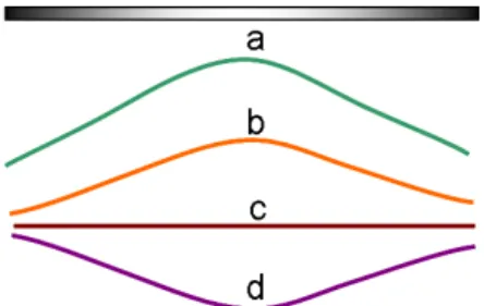
Figure 3.4: Using color to encode the Euclidean shortest distance between surfaces can by ambiguous. As a 2D example, the color bar on top can represent the distance between curveaand any of linesb, c, ord.

and metric value simultaneously [War88]. However, Ware was not investigating color maps on smooth

surfaces, but rather smooth univariate maps in 2D images. Luminance is not available for mapping

metric values on smooth surfaces, because luminance is required to convey the surface shape (via

illumination).

In this study, two color scales are used. Both use hue to label the two ends of the scale. The first

scale interpolates saturation, passing through a desaturated grey between in the middle of the scale.

The second scale interpolates between the two end hues alone.

3.3.3 Cut-away Geometry

There are a number of very simple and frequently employed techniques which remove some

(42)

for how geometry is removed, so these techniques are not necessarily appropriate for direct use in

general layered-surface visualization.

One method of removing occluding geometry is to render some of the layered objects in wireframe

(only the edges of the polygonal facets of the surface geometry are actually rendered). Unfortunately,

this approach reveals more of the approximation to the surface than it reveals the represented shape

(see Figure 3.5). A common compromise is to use a simple texture with regular regions of

translu-cence, such as a grid (see Figure 3.6). This gives uniformity to the pattern of opacity and translucency

and enables the possibility of user control. However, finding non-distorted texture coordinates for

a surface of arbitrary topology is an area of active research, and I know of no technique that could

guarantee the regularity of the texture on an arbitrary surface.

Figure 3.5: Two intersecting surfaces are visualized. One surface is displayed as an opaque trian-gle mesh, and the second surface is displayed by the edges of the triantrian-gle mesh only (a technique commonly referred to aswireframe).

Two related methods are planar contours and ribbons. The planar contours technique reveals

the intersections of layered surfaces and a stack of evenly-spaced parallel planes. It can be difficult

to understand the full surface shape from these contours and more so to understand relationships

between surfaces between planes. Ribbon techniques are less aggressive at removing geometry than

planar contours. Instead of rendering only the planar intersections, only geometry between alternating

pairs of planes are removed. For instance, the geometry between every other pair of planes may be

(43)

Figure 3.6: Two intersecting surface are visualized. One surface is displayed as an opaque triangle mesh, and the second surface is displayed with a grid texture modulating the surface translucency.

Bauer-Kirpeset al.used a ribbon-like technique for displaying nested surfaces in medical applications

[BKSBL87] (see Figure 3.7). The technique bears some similarities to a technique proposed, but not

implemented, for this work (see Section 4.3).

Figure 3.7: The technique of Bauer-Kirpes et al. displays only ribbon-like pieces of the exterior surface, called “barrel hoops” [BKSBL87].

Diepstratenet al. describe techniques for automatically producing breakaway and cutaway

illus-trations of nested surfaces [DWE03] (see Figure 3.8). The automatic algorithm can be combined with

any non-photorealistic techniques to illustrate the interior of an otherwise solid object. A number of

potentially useful cutout styles are proposed. These illustrations remove portions of exterior geometry

(44)

Figure 3.8: This image shows examples of cutaway illustrations from Diepstratenet al.[DWE03].

None of these techniques are included for study in this work. They are all interesting techniques

for later comparison as part of future work.

3.3.4 Translucence

A common, simple, but perceptually ineffective method to display nested surfaces is to simply

render exterior surfaces with uniform translucency. Unfortunately, uniform translucency confounds

shape perception away from object silhouettes. Techniques that render occluding surfaces as a mix of

translucent and opaque materials generally enable better shape perception than uniform translucency.

Interrante provides an excellent summary of relevant perceptual issues for using translucency in

visualizations [IFP97]. The most critical aspect in perceiving that a surface is translucent is apparent

contrast reduction. For a surface to be perceived as translucent, the surface must reduce the apparent

contrast of the background while preserving relative brightness ordering. Metelli proposed a model

requiring an achromatic translucent surface to modulate background reflectance ratios consistently

[Met74]. D’Zmura found similar requirements for chromatic translucent layers [DRG00]. However,

these models do not explain translucent-layer perception in terms of the transmittance of the layer

itself. More recently, Singh found that perception of translucent layers must obey Michelson contrast

and that the Metelli and D’Zmura models both converge to Michelson contrast [Sin04].

Diepstratenet al. describe a technique for view-dependent translucency, which aims to

automat-ically produce translucent surfaces similar to technical illustrations [DWE02] (see Figure 3.9). The

technique is somewhat limited by the use of uniform translucency. Also, as with the Diepstraten

(45)

too much of the exterior will be rendered translucent to effectively perceive its shape.

Figure 3.9: This image shows an example of view-dependent transparency for technical illustration from Diepstratenet al.[DWE02].

Some successful techniques render an opaque interior surface surrounded by textured, translucent

exterior surfaces [IFP96, IFP97, Rhe96]. The texture patterns modulate local translucency, providing

better illumination and texture cues to enhance exterior surface shape perception as compared to

uniform translucency.

Rheingans re-tiled surfaces so that uniform circle or hexagon textures could be applied around

ver-tices [Rhe96]. Because the surface geometry is uniform, very simple texture patterns produce uniform

texture patterns that reveal shape effectively through texture compression (see Figure 3.10). Multiple

nested layers may be represented in different colors and even different simple texture patterns. The

simple textures tile the surface seamlessly and enable interactive display.

Figure 3.10: Rheingans retiled surfaces and applied simple translucency-modulating textures to con-vey shape of an exterior surface while enabling the interior surface to be seen as well [Rhe96].