DYNAMICS AND MIXING IN A MICROTIDAL, WIND-DRIVEN ESTUARY
David Marshall
A dissertation submitted to the faculty at the University of North Carolina at Chapel Hill in partial fulfillment of the requirements for the degree of Doctor of Philosophy in the Department
of Marine Sciences.
Chapel Hill 2018
iii ABSTRACT
David Marshall: Dynamics and mixing in a microtidal, wind-driven estuary (Under the direction of Johanna Rosman)
iv
ACKNOWLEDGEMENTS
I would like to thank my advisor, Johanna Rosman, for her help and guidance throughout the course of my graduate career. I would also like to thank my committee members: Jim Hench, Rick Luettich, John Bane, and Harvey Seim for always asking tough questions and making me think deeper about my research. To Tony Whipple, Ryan Neve, and Yu Xiao, thank you for your help in conducting the field measurements for this research.
Finally, this work would not have been possible without financial support from the NCDEQ Coastal Recreational Fishing License Grants program, the National Science Foundation (Physical Oceanography program OCE-1061108, OCE-1435530), University of North Carolina at Chapel Hill Department of Marine Sciences and Graduate School and the Mills Brown
Memorial Trust. The field measurements conducted for this dissertation were funded by NCDEQ Coastal Recreational Fishing License Grants program, the University of North Carolina at
v
TABLE OF CONTENTS
LIST OF FIGURES………..viii
SUMMARY……….1
CHAPTER 1: MOMENTUM AND SALT BUDGETS IN A WIND-DRIVEN, MICROTIDAL ESTUARY………...3
Introduction………..3
Methods.………...9
Field Site………..9
Field Measurements………...10
Data Processing………..11
Results………14
Experimental Conditions………14
Cross-sectionally averaged momentum budget………..15
Two-layer momentum budget………...20
Salt Flux……….27
Discussion………..31
vi
Chapter 1 Figures………...37
References………..53
CHAPTER 2: TURBULENT MIXING IN A STRATIFIED, MICROTIDAL, WIND-DRIVEN, ESTUARY……...………...56
Introduction………56
Theoretical Framework………..58
Turbulent Kinetic Energy Equation………58
Turbulent Length Scales……….60
Dimensionless Numbers……….62
Mixing Efficiency……….. 64
Methods………..65
Field Measurements………...65
Data Processing………..67
Calculation of turbulence statistics……….69
Results and Discussion………...72
Experimental Conditions………72
Turbulent Kinetic Energy Budget………...73
Turbulence Length Scales………..75
vii
viii
LIST OF FIGURES
Figure 1.1 – Bathymetric map of Neuse River Estuary……….37
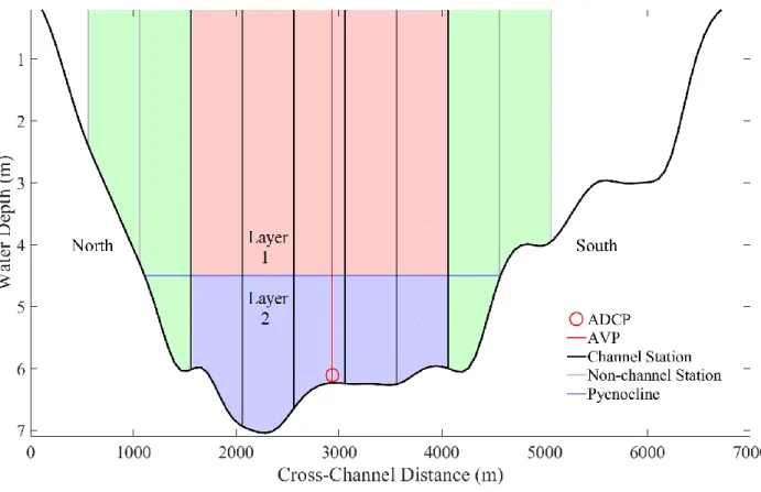
Figure 1.2 – Cross-section of Neuse River Estuary………...38
Figure 1.3 – Conditions during deployment………..39
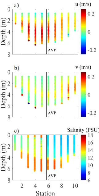
Figure 1.4 – Average shipboard ADCP/CTD profiles………...40
Figure 1.5 – Terms of the cross-sectionally averaged momentum budgets………...41
Figure 1.6 – Multi-taper spectra of the cross-sectionally averaged momentum budget terms…..42
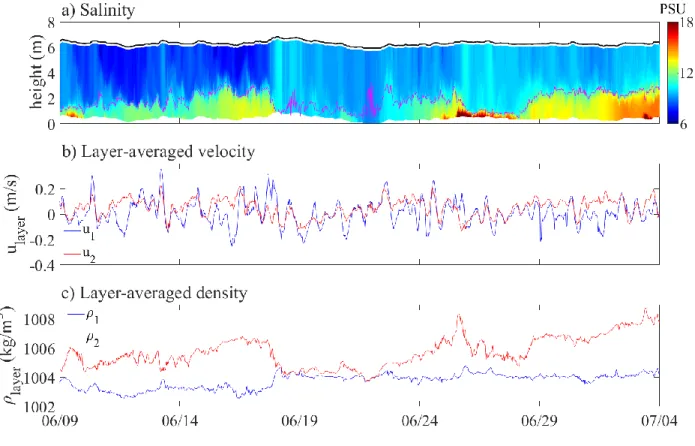
Figure 1.7 – Layer-averaged velocity and density……….43
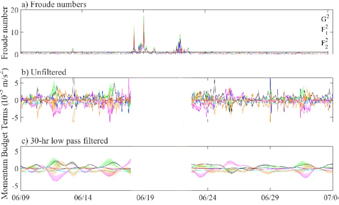
Figure 1.8 – Time series of internal and layer Froude numbers………44
Figure 1.9 – Multi-taper spectra of the terms in the two-layer momentum budget………...45
Figure 1.10 – Time series of wind stress, freshwater and volumetric flow rates, and S0………..46
Figure 1.11 – Cross-sectional estimates of uE and sE ………47
Figure 1.12 – Time series of salt flux and total salt content………..48
Figure 1.13 – Response of the estuary to a typical up and down-estuary wind……….49
Figure 1.14 – Time series of horizontal Righardson number, g’, and mixing number…………..50
Figure 1.15 – Variation of g’ and ∆g’, and mixing number………..51
Figure 1.16 – Estuarine parameter space………...52
Figure 2.1 – Map of Neuse River estuary showing the location of the study site……….84
ix
Figure 2.3 – Example power spectrum of vertical velocity from an ADV………86
Figure 2.4 – Cospectrum of along-channel and vertical velocity components………..87
Figure 2.5 – Wind direction, salinity, along-channel and across-channel current profiles……...88
Figure 2.6 – Profile of logarithm of normalized gradient Richardson numbers………89
Figure 2.7 – Histograms of N2 and S2 ………...90
Figure 2.8 – Histograms of dissipation, production, buoyancy flux, and turbulent kinetic energy.………91
Figure 2.9 – Time series of dissipation, production, and buoyancy fluxes………...92
Figure 2.10 – Production versus dissipation, ad buoyancy flux versus dissipation………...93
Figure 2.11 – Histograms of important turbulent length scales……….94
Figure 2.12 – Time series of Kolmogorov, Ozmidov, Corrsin, and Ellison length scales………95
Figure 2.13 – Time series of turbulent kinetic energy and turbulent length scales………...96
Figure 2.14 – Flux Richardson number versus buoyancy Reynolds number………97
Figure 2.15 Turbulent Froude number – Turbulent Reynolds number diagram………98
1 SUMMARY
Most previous work on the physical processes in estuaries has focused on tides as the primary mixing mechanism. However, there is a family of microtidal estuaries, driven primarily by the wind, which are not as well understood. Due to the episodic nature of the wind, vertical mixing is often weak, resulting in strong salinity stratification. In this dissertation, field studies were conducted to investigate the effects of time-varying, unsteady winds on circulation, salt transport and turbulent mixing in the Neuse River Estuary, one of these microtidal, wind-driven estuaries in eastern North Carolina.
The focus of the first field study was to investigate the circulation and salt transport in the Neuse. An analysis of the depth-averaged momentum equation demonstrated that the primary balance was between the wind stress and barotropic pressure gradient, indicating the presence of a wind-generated barotropic seiche. During periods of strong stratification, there was a two-layer circulation pattern, in which the wind stress was balanced by a combination of the interfacial stress, bottom stresses, and interfacial tilt. Up-estuary winds reduced the stratification and reduced or reversed the exchange flow, briefly causing a net transport of salt into the estuary until the water column became vertically mixed. Down-estuary winds enhanced the exchange flow and increased stratification, except when the wind stress was strong enough to overcome stratification and directly mix the water column. This asymmetric response to the predominantly down-estuary winds enhanced exchange flow, which when combined with a decrease in
2
A new set of parameters were defined in order to compare the physics of a wind-driven estuary to classical tidal estuaries. Due to a wide range of wind speeds and durations, the Neuse
experiences varying amounts of mixing, and thus can be classified differently, depending on the wind conditions. Strong winds resulted in well-mixed conditions, while weak winds generally resulted in strongly stratified conditions. Straining by moderate down-estuary winds caused the Neuse to behave like a wind-induced SIPS estuary.
In a second field study in the Neuse, we observed some of the strongest stratifications reported in estuaries, yet high turbulent dissipation rates. However, the observed turbulence was scarce and estimates of turbulent length scales indicated that the overturns were often so small that it was difficult to quantify the effects buoyancy and shear on turbulence properties. Application of a recently proposed framework suggested that some of the observed turbulence fell into an inertia-dominated regime, in which the turbulence was decaying, and eddies were no longer large enough to be affected by buoyancy or shear. Dissipation was generally larger than production and the mixing efficiencies associated with this turbulence were generally quite small. Turbulent mixing was more efficient in the shear and buoyancy-dominated regimes. The observed turbulence in this study was generated by two distinct mechanisms: shear generation, associated with advection of a salt wedge, and wind mixing. The turbulence
3
CHAPTER 1: MOMENTUM AND SALT BUDGETS IN A WIND-DRIVEN, MICROTIDAL ESTUARY
Introduction
Estuaries are complex systems, driven by a variety of mechanisms, including freshwater flow, tides, and wind, which can produce energetic turbulence and strong density gradients. Averaging over short term variations in velocity, such as those produced by tides, reveals that estuaries are characterized by an exchange flow, in which there is a persistent outflow (seaward) at the surface and a persistent inflow (landward) near the bottom. This exchange flow transports salt to the coastal ocean at the surface, while importing salt near the bottom. Vertical mixing is important in maintaining the estuarine circulation and salt flux, as mixing affects the strength of the exchange flow.
Most previous work on estuarine circulation has focused on tides as the primary mixing mechanism (reviewed by MacCready and Geyer 2010, Geyer and MacCready 2014). Budgets of momentum and salt in these tidal systems have been studied extensively, dating back to Hansen and Rattray (1965). Despite the complexities of estuarine circulation, which include nonlinear coupling of velocity and density structures, classical analyses often simplify momentum and salt budgets to a single cross-section. In doing so, it is assumed that the along-channel variation in bathymetry is negligible, and the along-channel salinity gradient is constant over the cross-section.
4
viscosity and vertical shear. This along-channel momentum budget can be further simplified to a one-layer model, by integrating the momentum equation over the water depth. The only stress terms that remain are the bottom stress and surface wind stress. In fact, wind is traditionally ignored, so the only the bottom stress retained in a one-layer model. Although a one-layer model is often appropriate for well-mixed and some partially mixed estuaries (e.g., Chatwin, 1976), where the along-channel salinity gradient drives the exchange flow, in strongly stratified and salt wedge estuaries, the stress between the surface outflow and bottom inflow can have a large effect on the dynamics. To resolve the exchange flow, a two-layer model can be constructed by
dividing the water column into two layers and then computing momentum balances for each layer (Geyer, 2000; Geyer and Ralston, 2011). An equation describing the dynamics of the exchange flow is obtained from the difference between the top and bottom layer momentum budgets. The differential flow between the top and bottom layers is driven entirely by the baroclinic pressure gradient, since the barotropic pressure gradient affects both layers equally and is eliminated by subtraction.
Because of the dynamical importance of the baroclinic pressure gradient term, the estuarine momentum budget is strongly coupled with the salt budget. As cast in Lerczak (2006), the salt budget consists of three terms: the salt loss due to river flow, the salt flux due to
exchange flow, and tidal salt flux which has the form of a dispersion term. Increasing river flow pushes the salt intrusion seaward and increases the horizontal salinity gradient. The magnitude of this increase in along-estuary salinity gradient depends on the responses of the exchange flow and tidal salt fluxes to the increase in horizontal salinity gradient.
strain-5
induced periodically stratification (SIPS), occurs when tidal variations in vertical shear drive tidal variations in stratification (tidal straining). Hence, tidal variations in vertical mixing have an important effect on the exchange flow (Simpson, 1990). The ratio of potential energy generation due to straining of the density field by velocity shear in the bottom boundary layer during ebb tide to production of turbulent kinetic energy by mixing in the bottom boundary layer is traditionally quantified by the horizontal Richardson number (Simpson, 1990)
𝑅𝑖𝑥 =𝐻
2𝑁 𝑥2
𝑢∗𝑏2 (1.1)
where H is the water depth, u*b is the bottom friction velocity, 𝑁𝑥2 = 𝑔 𝜌0
𝜕〈𝜌̅〉
𝜕𝑥 , g is the gravitational
acceleration, 0 is a constant reference density, and 〈𝜌̅〉 is the cross-sectionally averaged density.
When Rix is small, mixing in the boundary layer destroys stratification, leading to a well-mixed water column. High values of Rix lead to runaway stratification, as straining generates
stratification that cannot be mixed by bottom boundary layer turbulence. In SIPS estuaries, Rix takes intermediate values, as the water column becomes stratified during ebb tides and well mixed during flood tides (Geyer and MacCready, 2014).
In order to quantify the effectiveness of mixing at the bottom boundary, it is necessary to compute both the strength of the turbulent mixing and the time period over which that mixing occurs, because the bottom boundary layer grows in height over a tidal cycle. Despite its merits, Rix accounts for the strength, but not the time scale of mixing, and therefore is not suitable for
explaining how much of the water column becomes mixed. Geyer and MacCready (2014) parameterized the growth of the bottom boundary layer analogously to the growth of a wind-mixed layer:
𝑑ℎ𝐵𝐿 𝑑𝑡 = 𝐶
𝑢∗𝑏2
6
where hBL is the height of the bottom boundary layer, N is the stratification above the bottom boundary, and C 0.6 is a constant related to the mixing efficiency (Kato and Phillips, 1969; Trowbridge, 1992). They define a mixing number, M to determine the conditions in which the bottom boundary layer will extend into the entire water column within a half tidal cycle.
𝑀2 = 𝑢∗𝑏
2
𝜔𝑁0𝐻2 (1.3)
where 𝑁0 = √βg𝑠𝑜𝑐𝑒𝑎𝑛/𝐻 is the buoyancy frequency for maximum top-to-bottom salinity
variation in an estuary, is the coefficient of saline contraction, socean is the salinity of ocean water, and is the tidal frequency. A mixing number 𝑀 ≥ 1 corresponds to bottom boundary layer growth to entire water column in a half tidal cycle. Geyer and MacCready (2014) proposed an estuarine classification scheme based on tidal mixing (M), and the freshwater inflow (Frf). Here 𝐹𝑟𝑓 = 𝑢𝑅/√βg𝑠𝑜𝑐𝑒𝑎𝑛𝐻, is the freshwater Froude number which represents the ratio of river
inflow to strength of the gravitational circulation and 𝑢𝑅 is the velocity due to freshwater flow.
By placing estuaries in Frf –M parameter space (Fig. 1.16), they can be classified as salt wedge (e.g., Mississippi, Ebro), time dependent-salt wedge (e.g., Frasier, Merrimack), strongly stratified (e.g., Chesapeake, Hudson), partially stratified (e.g., James, San Francisco Bay), SIPS (e.g., Conwy, Willapa Bay), fjord (e.g., Puget Sound, Long Island Sound), or bay (e.g., Narragansett Bay). Several estuaries (e.g., Hudson, Chesapeake, San Francisco Bay) span partially mixed and strongly stratified, salt wedge, or SIPS during the spring-neap cycle.
7
mixing and circulation patterns (e.g., Luettich et al., 2002). Unlike tides, the wind is inherently irregular and episodic, making it much more difficult to express the estuarine dynamics with simple models.
Much of what is known about the dynamics of shallow wind-driven systems originates from the study of stratified lakes (e.g., Spigel and Imberger, 1980; Bouffard et al., 2012).
Unsteady winds can initiate barotropic and baroclinic motions by changes in wind forcing, which can continue to contribute to advection and modify stratification after a wind event. Wind
blowing over the surface of a lake both generates a turbulent, wind-mixed layer and induces a vertically sheared circulation pattern that results in tilts of both the water surface and isopycnals. The relative strengths of the maximum baroclinic pressure gradient force associated with a fully titled pycnocline and the force due to the surface wind stress can be quantified by the
Wedderburn number (Thompson and Imberger, 1980; Monismith, 1985)
𝑊 = 𝑔′ℎ1 𝑢∗𝑤2𝐿
(1.4) where g’ is the reduced gravity, h1 is the height of the surface wind-mixed layer, u*w is the
wind-generated surface friction velocity, and L is the length of the water body. The Wedderburn number is a measure of whether complete upwelling will occur. When W > 1, mixed layer deepening does not affect the baroclinic seiche motions (Spigel and Imberger, 1980). When W < 1, unsteady interfacial shear stress contributes to mixing. If the winds become strong enough (W << 1), the mixed layer deepens from the surface to the bottom and the lake is no longer stratified.
8
drives vertically sheared flow with the strongest speeds typically near the surface, enhancing stratification for down-estuary winds and reducing stratification for up-estuary winds (Geyer, 1997; Scully et al. 2005). These effects on stratification feed back to the mixing (Chen and Sanford 2009). Stronger stratification during down-estuary winds limits mixing and supports larger vertical shear than when winds are directed up-estuary. Chen and Sanford (2009) defined a modified version of the horizontal Richardson number to characterize the relative importance of straining and mixing, due to the combined effects of tides and wind. They found that this
parameter was able to capture how the stratification increased and then decreased with increasing down-estuary winds. From observations in Chesapeake Bay, Xie and Li (2018) found an
asymmetric stratification response, in which stratification decreased linearly with W for up-estuary winds, but stratification was a parabolic function of W for down-up-estuary winds,
increasing at moderate wind speeds and decreasing at high wind speeds. Changes in wind speed or direction have also been found to result in large transient salt fluxes (Chen and Sanford, 2009).
A recent study of a lagoonal estuary using a 3-D hydrodynamic model has given some insights into the circulation dynamics of estuaries that are not just modulated, but driven by the wind (Jia and Li, 2012). They found that the circulation was primarily driven by a balance
between the total pressure (barotropic plus baroclinic) gradient and stress divergence (wind stress minus bottom stress). They also found that the baroclinic forcing was highly asymmetric
between up-estuary and down-estuary winds, which supports the findings of other studies that the wind can strain the density field.
9
to which these findings can be applied to real strongly stratified, wind-driven estuaries. This study used field measurements to investigate the effects of time-varying, unsteady winds on circulation and salt transport in a wind-driven estuary. We investigate whether the findings of the modeling studies (Chen and Sanford, 2009; Jia and Li, 2012) that wind can both strain and mix the water column are important in a real estuary. Secondly, we investigate whether the
frameworks (one and two-layer momentum budgets, salt budgets, and the Frf –M parameter space) that have been used to understand and classify tidally mixed estuaries can also be used to understand a system where wind is the primary agent driving mixing and short time-scale advection.
Methods Field Site
The Neuse River Estuary (NRE), in eastern North Carolina, is a shallow, microtidal estuary, driven largely by wind and freshwater discharge. The estuary is approximately 70 km long, with a mean width of about 6.5 km, a mean depth of about 3.5 m, and a prominent bend approximately mid-estuary (Fig. 1.1). The NRE connects to Pamlico Sound, a large, lagoonal estuary, which is isolated from the Atlantic Ocean by the Outer Banks barrier islands, except for limited tidal exchange through three small inlets. While the NRE has weak tidal influence and low freshwater discharge, its large fetch allows wind to be the main driver of flow patterns and turbulent mixing. The prevailing wind direction is northeast – southwest, aligned with main axis of the lower Neuse. During the summer, the NRE becomes episodically strongly salinity
10
from wind-driven barotropic seiches with a period of about 13 hours (Luettich et al., 2002). Typical depth-averaged oscillatory velocities are about 10 cm/s.
Field Measurements
The study was conducted over a one-month period from June 9 to July 4, 2016 in the lower part of the NRE. We deployed an array of sensors at three sites along the main channel from the bend in the estuary to the mouth of Pamlico Sound (Fig. 1.1). The instruments at the bend and central sites were deployed in the deepest part of the channel, while those at the mouth were deployed on a shoal for logistical reasons.
At each of those sites, we made continuous measurements of currents and salinity with a bottom-mounted ADCP (Teledyne-RD Instruments 1.2-MHz Workhorse Monitor) and a vertical mooring of three CTDs (SeaBird SBE-37SMP). The ADCPs sampled every 1 second, and were deployed in fast-pinging rate mode, with 6 subpings per profile (mode 12; Nidzieko et al., 2006). Velocities were recorded in beam coordinates for the entire water column (6-7 m) in 25-cm vertical bins, the first of which was centered 1.5 m above bottom. At each mooring the lower CTD was located at 1 m above bottom, the middle CTD at half of the water depth, and the top CTD at 1.5 to 2-m below the water surface. The CTDs sampled at 5-minute intervals.
11
recorded wind speed and direction at 30-minute intervals. Additionally, hourly atmospheric pressure data were obtained from the Marine Corps Air Station at Cherry Point.
To quantify the cross-sectional spatial structure of salinity and currents, we made
measurements along transects at 10-12 equally-spaced stations (0.5 km apart) across the estuary at each of the three main sites in the Lower Neuse (Fig. 1.1). These shipboard measurements were collected on 5 days (6/20, 7/5, 7/18, 8/16, and 9/19), many of which extended beyond the main study period. Velocity profiles were measured with a boom-mounted (Hench et al., 2000) shipboard ADCP (1.2 MHz Workhorse, RD Instruments), and CTD profiles were made at the same stations (SBE19plus V2, Seabird Electronics). At each station ADCP data were collected for six minutes in mode 1, with 0.25 m bins and a ping rate of 1Hz, yielding an uncertainty of 0.0072 m/s. Although the vessel was nominally stopped at each station, the remaining vessel motion was removed using ADCP bottom tracking. At the same time, a single CTD cast was conducted with a sampling rate of 4 Hz.
Data Processing
The ADCP and CTD data were 30-minute ensemble averaged such that the middle of each interval coincided with the AVP profiles. Wind speeds at the AVP site collected at 5 m above the surface were transformed to 10-m wind speeds (for wind stress calculations) assuming an atmospheric log profile (Blanton et al, 1989). Both the ADCP velocity data and the wind velocity data were rotated into along- and across-channel directions, determined from the principal components of the depth-averaged ADCP velocities. To compute velocities averaged over the entire water column, velocities were extrapolated to the surface (0.5 m) assuming zero velocity gradient at the surface and a log-layer at the bottom of the water column. The
12
Depth-averaged values of salinity, temperature, and density were computed from the AVP profiles at the central site and from the CTD moorings at the bend and mouth sites. All three CTDs at the mouth site were in the top layer during periods of stratification, so values were extrapolated to the bottom of the channel by assuming that along-estuary gradients were constant throughout the entire water column. Thus, the magnitude of the vertical density gradient at the mouth was equal to the vertical density gradient at the central site.
Shipboard CTD measurements were averaged in 0.1 m bins, resulting in profiles with the same resolution as those collected by the AVP. These shipboard measurements were then used to estimate cross-sectionally averaged values of depth, velocity, salinity, and density based on the continuous measurements from the moored ADCP and AVP. First, depth-averaged values were computed for each station (both channel and non-channel stations in Fig. 1.2). An offset was assigned to each station by computing the difference between the value at that station and the value at the station closest to the moored instruments. For depth-averaged velocity, that is 𝑢̅𝑆𝑖 =
𝑢̅𝐶𝐿+ 𝜎𝑢𝑖, where 𝑢̅𝑆𝑖 is the depth averaged velocity at station i (i=1:10 for the bend and central
13
profiles. Finally, cross-sectional averages of velocity, salinity, and density were computed from the station-estimated values. For the cross-sectionally averaged velocity, 〈𝑢̅〉
〈𝑢̅〉 =∑ 𝑢̅𝑆𝑖𝐻𝑖𝑑𝑖
𝑁 𝑖=1
𝐴 (1.5)
where N is the number of stations, 𝐻𝑖 is the estimated depth at each station, computed by applying an offset to the depth at the location of the moored instruments, 𝑑𝑖 is the distance between stations, and A is the cross-sectional area. Cross-sectionally averaged values of salinity and density were computed from equations of the same form as equation 1.5. Using centerline values and assuming horizontal isotachs resulted in estimates of cross-sectionally averaged velocities that were an average of about 1 cm/s (20 %) slower than those computed using offsets derived from the shipboard measurements, in which the isotachs were not horizontal.
Uncertainties were estimated for velocity, density, wind speed, and water depth measurements for each 30-minute interval. These uncertainties were used to calculate the uncertainties in the terms of the momentum budgets via a propagation of uncertainty formula (Taylor, 1996). The standard deviation the mode-12 ADCP velocities was 1.44 cm/s (Teledyne RD Instruments, 2006). Ensemble averaging over 30-minute intervals resulted in a standard error of 8 x 10⁻⁴ m/s. The instrument error in a salinity measurement was 1% (YSI Incorporated, 2017), which corresponded to a density error of 0.2 kg/m3. Assuming an average of 10 salinity measurements per 10-cm bin, the density error for each bin was 0.06 kg/m3. The uncertainties in
14 Results
Experimental conditions
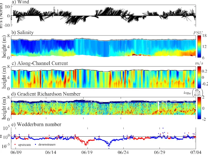
During the study period, winds were typically oriented along the axis of the estuary (NE-SW direction) (Fig. 1.3a). The lower Neuse was strongly stratified by salinity for the majority of the field experiment (Fig. 1.3b), except during periods of strong winds. During periods when the water column was stratified, profiles of along-channel velocity were strongly vertically sheared. The current at the surface was generally aligned with the wind direction (Fig. 1.3c).
The average shipboard measurements for the central site are shown in Fig. 1.4. The channel was typically strongly stratified by salinity (Fig. 1.4c), although stations on the shoals were often so shallow that they only contained the top layer. As a result only the six stations in the middle of the channel were used when computing the two-layer model (Fig. 1.2). The largest vertical shears in the along-channel (Fig. 4 a) and cross-channel (Fig. 1.4b) directions were typically co-located with the pycnocline.
During periods of strong stratification, the gradient Richardson numbers which were typically greater than 0.25 near the pycnocline (Fig. 1.3d), indicating that the flow was stable. However, near the surface and bottom, Rig < 0.25. Periods of weak stratification, which were
associated with strong winds, resulted in more uniform velocity profiles, and Rig <0.25
15
Time series of the Wedderburn number (Fig. 1.3e) show that the wind stress was large relative to the maximum achievable baroclinic pressure gradient force (W<<1), indicating that wind stress was an important forcing mechanism. Weak down-estuary winds enhanced the stability by straining the water column and increasing exchange flow (Fig. 1.3 a-c). However, when the down-estuary wind was sufficiently strong (June 21-23), Richardson numbers were less than 1/4 throughout the water column indicating that shear was sufficient to overcome the
stratification and mix the water column. Up-estuary wind events acted against the estuarine exchange flow, causing the exchange flow to reverse, before disappearing altogether as the water column mixed and the velocity uniform throughout the water column (June 17-20, 26-28).
Cross-Sectionally Averaged Momentum Budget
To understand the underlying mechanisms driving the kinematical characteristics of an estuary, the dynamics were explored through the analysis of the momentum budget in the along-channel direction, which is given by:
𝜕𝑢 𝜕𝑡 + 𝑢
𝜕𝑢 𝜕𝑥+ 𝑣
𝜕𝑢 𝜕𝑦+ 𝑤
𝜕𝑢
𝜕𝑧− 𝑓𝑣 + 1 𝜌0
𝜕𝑝 𝜕𝑥−
1 𝜌0(
𝜕𝜏𝑥𝑥 𝜕𝑥 +
𝜕𝜏𝑥𝑦
𝜕𝑦 + 𝜏𝑥𝑧
𝜕𝑧) = 0 (1.6) where x is the along-channel direction with positive values in the upstream direction, u is the along-channel velocity, v is the cross-channel velocity, f = 8.34 x 10⁻⁵ s-1 is the local Coriolis parameter, and xx, xy, and xz are the Reynolds stresses, 𝜌(𝑢̅̅̅̅̅̅), 𝜌(𝑢′𝑢′ ̅̅̅̅̅̅), 𝜌(𝑢′𝑣′ ̅̅̅̅̅̅). The ′𝑤′
pressure gradient, p/x can be decomposed to express the influence of the surface slope and the horizontal density gradient:
1 𝜌0
𝜕𝑝 𝜕𝑥= 𝑔
𝜕𝜂 𝜕𝑥+
𝑔 𝜌0∫
𝜕𝜌
𝜕𝑥𝑑𝑧 (1.7)
cross-16
section, and dividing by the cross-sectional area. Following Speer (1985), the cross-sectionally averaged momentum equation is:
𝜕〈𝑢̅〉 𝜕𝑡 + 〈𝑢̅〉
𝜕〈𝑢̅〉 𝜕𝑥 + 𝑔
𝜕𝜂 𝜕𝑥+
𝑔
𝐴𝜌0∫ ∫ 𝜕𝜌 𝜕𝑥𝑧𝑑𝑧 𝜂 −ℎ 𝑑𝑦 𝑏2 −𝑏1
− 𝑓〈𝑣̅〉 +𝜏𝑏𝑥𝑃 〈𝜌̅〉𝐴−
𝜏𝑤𝑥
〈𝜌̅〉𝐻= 0 (1.8) where the overbar and brackets represents a cross-sectional average, h is the local water depth, and H is the cross-sectionally averaged water depth, A is the cross-sectional area, P is the wetted perimeter, bx is the along-channel bottom stress, and wx is the along-channel surface wind stress. The limits of integration, b1 and b2, are the y-coordinates at the two shores, such that the width of the estuary, B = b1 + b2.
In deriving the terms in equation 1.8, Speer (1985) assumed that the horizontal density gradient was negligible and thus ignored the fourth term in the equation. However, this term may be important in the present study site., Here we derive the full cross-sectionally averaged
baroclinic pressure gradient term. Applying Leibniz’s rule,
𝑔 𝐴𝜌0
∫ ∫ 𝜕𝜌 𝜕𝑥𝑧𝑑𝑧 𝜂 −ℎ 𝑑𝑦 = 𝑏2 −𝑏1 𝑔 𝐴𝜌0 [ 𝑑
𝑑𝑥∫ ∫ 𝜌𝑧𝑑𝑧
𝜂
−ℎ
𝑑𝑦
𝑏2
−𝑏1
−𝜕𝑏2
𝜕𝑥 ∫ 𝜌𝑏2𝑧𝑏2𝑑𝑧
𝜂
−ℎ
+𝜕(−𝑏1)
𝜕𝑥 ∫ 𝜌𝑏1𝑧𝑏1𝑑𝑧
𝜂
−ℎ
+ ∫ 𝜌(𝜂)𝜂𝜕𝜂 𝜕𝑥𝑑𝑦
𝑏2
−𝑏1
+ 𝑑
𝑑𝑥∫ 𝜌(−ℎ)ℎ
2𝑑𝑦 𝑏2
−𝑏1
+𝜕𝑏2
𝜕𝑥 𝜌(−ℎ𝑏2)ℎ𝑏2 2
−𝜕𝑏1
𝜕𝑥 𝜌(−ℎ𝑏1)ℎ𝑏1 2
]
(1.9)
Here, b1 and b2 appear as subscripts to indicate quantities at y = b1 or y=b2. The fourth term is approximately zero, assuming 𝜂 ≪ ℎ. If there is a gradual slope in the cross-channel direction, the depth at the boundaries is approximately zero, so terms 2, 3, 6, and 7 are zero. The baroclinic pressure gradient term reduces to:
𝑔 𝐴𝜌0
∫ ∫ 𝜕𝜌 𝜕𝑥𝑧𝑑𝑧
𝜂
−ℎ
𝑑𝑦 = 𝑔 𝐴𝜌0
[𝑑
𝑑𝑥∫ ∫ 𝜌𝑧𝑑𝑧
𝜂
−ℎ
𝑑𝑦 + 𝑑
𝑑𝑥∫ 𝜌(−ℎ)ℎ
17
Both terms on the RHS were estimated using the shipboard measurements from 5 transects (June to September, 2016), The last term was 2 orders of magnitude smaller than the first, so the baroclinic term can be reduced to:
𝑔 𝐴𝜌0
∫ ∫ 𝜕𝜌 𝜕𝑥𝑧𝑑𝑧
𝜂
−ℎ
𝑑𝑦 = 𝑔 𝐴𝜌0
𝑑
𝑑𝑥∫ ∫ 𝜌𝑧𝑑𝑧
𝜂 −ℎ 𝑑𝑦 𝑏2 −𝑏1 𝑏2 −𝑏1 (1.11)
Next, let 𝜌 = 〈𝜌̅〉 + 𝜌̅ + 𝜌̇, where 〈𝜌̅〉 is the cross-channel averaged density, 𝜌̅ is the depth averaged and width varying density, and 𝜌̇ is the depth and width varying density:
𝑔𝑑
𝐴𝜌0𝑑𝑥∫ ∫ 𝜌𝑧𝑑𝑧
𝜂 −ℎ 𝑑𝑦 𝑏2 −𝑏1 = 𝑔 𝐴𝜌0 [𝑑
𝑑𝑥∫ ∫ 〈𝜌̅〉𝑧𝑑𝑧
𝜂 −ℎ 𝑑𝑦 𝑏2 −𝑏1 + 𝑑
𝑑𝑥∫ ∫ 𝜌̅𝑧𝑑𝑧
𝜂 −ℎ 𝑑𝑦 𝑏2 −𝑏1 + 𝑑
𝑑𝑥∫ ∫ 𝜌̇𝑧𝑑𝑧
𝜂 −ℎ 𝑑𝑦 𝑏2 −𝑏1 ] = 𝑔 2𝐴𝜌0[𝐵𝐻
2𝑑〈𝜌̅〉
𝑑𝑥 + 𝑑
𝑑𝑥∫ 𝜌̅ℎ
2𝑑𝑦 𝑏2
−𝑏1
+ 2 𝑑
𝑑𝑥∫ ∫ 𝜌̇𝑧𝑑𝑧
𝜂
−ℎ
𝑑𝑦
𝑏2
−𝑏1
] (1.12)
Estimating the cross-sectionally averaged term (first term on the RHS of equation 1.12) and the full depth integrated term (LHS of equation 1.12) from the shipboard data indicated that the cross-sectionally averaged term accounted for approximately 1/3 of the baroclinic pressure gradient. This difference in baroclinic pressure gradient estimates may be due to large
uncertainty introduced by averaging values measured two-weeks apart, as well as estimating the cross-channel gradients from stations that were 0.5 km apart. To account for the difference, a Boussinesq coefficient, β = 3, was applied to the cross-sectionally averaged baroclinic pressure gradient term to get a better estimate of the total contribution of the baroclinic pressure gradient. That is:
𝑔 𝐴𝜌0
𝑑
𝑑𝑥∫ ∫ 𝜌𝑧𝑑𝑧
𝜂 −ℎ 𝑑𝑦 𝑏2 −𝑏1 ≈ 𝛽𝑔 2𝐴𝜌0𝐵𝐻
2𝑑〈𝜌̅〉
18
A similar empirical coefficient could be applied to each of the terms in equation 1.8, however, the shipboard measurements indicated that the differences between the terms computed using measurements at the centerline, multiplied by the sectional area, and the true cross-sectionally averaged terms were negligible.
Assuming that A BH, the cross-sectionally averaged momentum equation becomes: 𝜕〈𝑢̅〉
𝜕𝑡 + 〈𝑢̅〉 𝜕〈𝑢̅〉
𝜕𝑥 + 𝑔 𝜕𝜂 𝜕𝑥+
𝛽𝑔 2𝜌0
𝜕〈𝜌̅〉
𝜕𝑥 𝐻 − 𝑓〈𝑣̅〉 + 𝜏𝑏𝑥𝑃 〈𝜌̅〉𝐴−
𝜏𝑤𝑥
〈𝜌̅〉𝐻= 0 (1.14) The terms on the left-hand side are the local acceleration, the nonlinear advective acceleration, the barotropic pressure gradient force, the baroclinic pressure gradient force, the Coriolis acceleration, the bottom stress, and the wind stress.
To compute the barotropic pressure gradient term, the baroclinic contribution to the pressure measurements recorded by the ADCPs was first removed using a method similar to Geyer et al. (2000). First, the depth-integrated density, derived from AVP profiles, was used to compute the total pressure, and subsequently the height of the water column. was computed at each site by subtracting off the time-averaged water column height (averaged over the course of the entire field study). Finally, the free surface gradient was computed at the central site from the pressure measurement recorded by all three ADCPs, using second-order central differencing
𝑑𝜂 𝑑𝑥=
((𝑥𝑐𝑒𝑛𝑡− 𝑥𝑏𝑒𝑛𝑑)𝜂𝑥𝑚𝑜𝑢𝑡ℎ− 𝜂𝑐𝑒𝑛𝑡
𝑚𝑜𝑢𝑡ℎ− 𝑥𝑐𝑒𝑛𝑡 + (𝑥𝑚𝑜𝑢𝑡ℎ− 𝑥𝑐𝑒𝑛𝑡)
𝜂𝑐𝑒𝑛𝑡 − 𝜂𝑏𝑒𝑛𝑑 𝑥𝑐𝑒𝑛𝑡 − 𝑥𝑏𝑒𝑛𝑑)
(𝑥𝑚𝑜𝑢𝑡ℎ − 𝑥𝑏𝑒𝑛𝑑)
(1.15)
19
The surface wind stress in the along-estuary direction was estimated using wind data from the AVP’s anemometer and assuming a parabolic model of the drag coefficient of the form 𝐶𝐷𝑤= −𝐴(𝑈10− 33)2 − 𝑐 (Peng and Li, 2015). Here, CDw is the drag coefficient associated
with the surface wind stress, U10, is the wind speed 10 m above the surface, and A = 7 x 10⁻⁷ and c = 2.34 x 10⁻³ are empirical coefficients. Over the course of the study CDw ranged from 1.6 x 10 -3 to 2.1 x 10⁻³. The bottom stress in the along-channel direction was estimated using a quadratic
drag law: 𝜏𝑏𝑥 = 𝜌𝐶𝐷|𝑢𝑏𝑥|𝑢𝑏𝑥, where 𝐶𝐷 is the bottom drag coefficient and 𝑢𝑏𝑥 is the near bottom along-channel velocity. Here, 𝐶𝐷 is assumed to be 2.5 x 10⁻³, which is typical of sand-bottomed estuaries, (Proudman, 1953; Prandle, 2003) and 𝑢𝑏𝑥 is the along-channel velocity in
the first bin recorded by the ADCP (about 1.5 m above bottom).
20
seiche signal dominates the momentum budget, and appears as a balance between the local acceleration term and the barotropic pressure gradient term (Fig. 1.5 c,e).
Multi-taper spectra of each term were computed to further understand these balances (Fig. 1.6). Low frequencies are dominated by the barotropic pressure gradient (green) and wind stress (pink) terms. At intermediate frequencies there is a balance between the barotropic pressure gradient and local acceleration. The highest frequencies (periods < 6 hours) are
dominated by the wind stress, barotropic pressure gradient, local acceleration, and residual terms terms (Fig. 1.6), as unsteady winds accelerate the water for brief periods of time and generate transient gradients in the water surface.
Two-layer momentum budget
Throughout most of the measurement period, the water column consisted of two layers with distinctly different salinities, separated by an interface of varying thickness. We therefore decided to apply a two-layer model to better understand the dynamics. A two-layer model is most appropriate if the widths of both layers are approximately equal. Due to the shape of the central cross-section, the two-layer model was therefore only applied to the channel, which was defined as the area between the middle six shipboard stations (Fig. 1.2).
To further determine the validity of a two-layer model, it is important to consider the hydraulics of the system. The hydraulics of the two-layer system are described by the composite Froude number:
𝐺2 = 𝐹12+ 𝐹22 = 𝑢1
2
𝑔′ℎ1
+ 𝑢2
2
𝑔′ℎ2
(1.16)
where 𝐹1 and 𝐹2 are the layer Froude numbers (Armi and Farmer, 1986). When G2 < 1, the flow
21
and the two-layer model is not appropriate. Together, G2 and g’ were used to determine when the two-layer model was applicable. Time series of the Froude numbers (Fig. 1.8a) and g’ (Fig. 1.14c) indicated that a two-layer model was not appropriate for a 5-day period between 6/18 and 6/23, where the flow was either supercritical or the water column was well-mixed. The two-layer momentum budget was therefore not applied during this period (Fig. 1.8 b-c).
The water column was divided into two layers by defining the interface as the height above bottom at which the maximum vertical salinity gradient was observed. (Fig. 1.7a).
Velocities and densities were then averaged over each layer. Surface and bottom layer velocities often exhibited typical estuarine circulation, although during periods of strong winds, both layers had the same velocity (Fig. 1.7b). Layer-averaged densities indicate that stratification was strong for much of the field study, except for a 5-day period from 6/18 to 6/23 when strong winds mixed the water column (Fig. 1.7c).
Following Geyer and Ralston (2011), the along-channel momentum budget for each layer can be written as:
𝜕𝑢1
𝜕𝑡 + 𝑢1 𝜕𝑢1
𝜕𝑥 + 𝑔 𝜕𝜂 𝜕𝑥+
𝐶𝑖|𝑢1− 𝑢2|(𝑢1− 𝑢2)
ℎ1 = 0 (1.17)
𝜕𝑢2 𝜕𝑡 + 𝑢2
𝜕𝑢2 𝜕𝑥 + 𝑔
𝜕𝜂 𝜕𝑥+ 𝑔
′𝜕ℎ𝑖
𝜕𝑥 +
𝐶𝑖|𝑢1− 𝑢2|(𝑢1− 𝑢2) ℎ2
+𝐶𝐷|𝑢2|𝑢2 ℎ2
= 0 (1.18) where ℎ1 and ℎ2 are the heights of the upper and lower layers, 𝑢1 and 𝑢2 are the upper and lower layer velocities, 𝜌1 and 𝜌2 are the upper and lower layer densities, 𝑔′ =
𝑔(𝜌2−𝜌1)
𝜌0 is the reduced
gravity, 𝜕ℎ𝑖
𝜕𝑥 is the slope of the interface between the two layers, and 𝐶𝑖 is an interfacial drag
22 term, 𝑢∗𝑤
2
ℎ1 was added to the layer 1 equation. By restricting the two-layer model to stations in
which there were always two layers, the wind stress should not directly affect layer 2, nor should the bottom stress directly affect layer 1. Shipboard measurements indicated that the horizontal density gradient was approximately equal for both layers, so a baroclinic pressure gradient term, ∫𝜕𝜌𝜕𝑥𝑧𝑑𝑧, was included in each layer. The baroclinic pressure gradient in the top layer was integrated from the surface to h1 and in the bottom layer from h1 to H. Finally, a momentum sink
term was added to each layer to account for any momentum lost due to lateral exchange between the channel and the shoals. This momentum sink term is the Reynolds stress at the edge of the channel (y = B) and can be parameterized using an eddy viscosity, 𝐴𝐻:
𝑢′𝑣′
̅̅̅̅̅̅ = 𝐴𝐻
𝜕𝑢𝑖 𝜕𝑦 ≈ 𝐴𝐻
Δ𝑢𝑖
Δ𝑦 (1.19)
where Δ𝑢𝑖 is the difference in layer velocities between the channel and the shoal for each of the
two layers (i=1,2). Alternatively, the Reynolds stress can be parameterized with a drag coefficient, 𝐶𝑆1, such that 𝑢̅̅̅̅̅̅ = 𝐶′𝑣′
𝑆1Δ𝑢12. By equating the two parameterizations of the
Reynolds stress, we get:
𝐶𝑆1 = 𝐴𝐻
Δ𝑢1Δ𝑦 (1.20)
A mixing length model can be used as a scaling estimate for the horizontal eddy viscosity (Pope, 2000):
𝐴𝐻 = 𝑙𝑚2 Δ𝑢1
Δ𝑦 (1.21)
where 𝑙𝑚 is the mixing length. Replacing 𝐴𝐻 with the mixing length model,
𝐶𝑆1 =
𝑙𝑚2
23
Both 𝑙𝑚 and Δ𝑦 scale as the width of the shear layer between the channel and the shoal, so 𝐶𝑆1 ≈
1. Replacing 𝜕𝑦 with B in the top layer momentum equation, and using the drag coefficient parameterization, we have get the following layer-averaged equations:
𝜕𝑢1 𝜕𝑡 + 𝑢1
𝜕𝑢1 𝜕𝑥 + 𝑔
𝜕𝜂 𝜕𝑥+
𝐶𝑖|𝑢1 − 𝑢2|(𝑢1− 𝑢2)
ℎ1 −
𝑢∗𝑤2
ℎ1 + 𝑔ℎ1 2𝜌0
𝜕𝜌 𝜕𝑥+
2𝐶𝑠1|∆𝑢1|∆𝑢1
𝐵 = 0 (1.23) 𝜕𝑢2
𝜕𝑡 + 𝑢2 𝜕𝑢2
𝜕𝑥 + 𝑔 𝜕𝜂 𝜕𝑥+ 𝑔
′𝜕ℎ𝑖
𝜕𝑥 −
𝐶𝑖|𝑢1− 𝑢2|(𝑢1− 𝑢2)
ℎ2 +
𝐶𝐷|𝑢2|𝑢2
ℎ2 +
𝑔(𝐻 + ℎ1)
2𝜌0 𝜕𝜌 𝜕𝑥 +2𝐶𝑠2|∆𝑢2|∆𝑢2
𝐵 = 0 (1.24)
Δ𝑢𝑖 was estimated from the shipboard measurements by computing the difference between the last station in the channel and the first station outside of the channel at each end of the estuary (stations 2-3 and 8-9). The average values of |Δ𝑢1| and |Δ𝑢2| were 0.02 and 0.09 m/s
respectively, which are comparable to the magnitudes of the other velocities in the equation. Since 𝐶𝑆1
𝐶𝐷 ~ 𝐵
𝐻, the momentum sink term should be about the same order of magnitude as the other
terms in the equation.
Taking the difference between the two layer-averaged equations eliminates the barotropic pressure gradient term, resulting in the final two-layer expression of the baroclinic dynamics:
𝜕
𝜕𝑡(𝑢2− 𝑢1) + 𝑢2 𝜕𝑢2
𝜕𝑥 − 𝑢1 𝜕𝑢1
𝜕𝑥 + 𝑔
′𝜕ℎ𝑖
𝜕𝑥 – 𝐶𝑖|𝑢1− 𝑢2|(𝑢1− 𝑢2) ( 1 ℎ1+
1 ℎ2) +
𝐶𝐷|𝑢2|𝑢2
ℎ2 +|𝑢∗w|𝑢∗w
ℎ1
+ 𝑔𝐻 2𝜌0
𝜕𝜌̅ 𝜕𝑥−
2𝐶𝑠1|∆𝑢1|∆𝑢1
𝐵 +
2𝐶𝑠2|∆𝑢2|∆𝑢2
𝐵 = 0 (1.25) The terms on the left-hand side are the local differential acceleration between layers, the
24
To compute each of these terms, velocities and densities were estimated at each of the shipboard stations using the same offset method explained previously. However, instead of computing offsets for depth-averaged values, offsets were calculated for layer-averaged values. Density measurements from the AVP were used to divide the water column in two, at the depth of the maximum vertical salinity gradient, and it was assumed that the isopycnals were
horizontal across the channel. At the central site, this resulted in 20 different regions (2 for each of the 10 stations) over which velocities and densities could be estimated. However, the two-layer model requires that the widths of both two-layers be the same, so only the 6 stations in the channel (Fig. 1.2) were used to compute the layer-averaged velocities and densities. By restricting estimates of layer-averaged velocities to the channel, cross-sectional averaged estimates only differed from the centerline velocity estimates by 0.003 m/s (4 %).
The shear stress between two layers is defined as: 𝜕
𝜕𝑧𝑢
′𝑤
̅̅̅̅̅̅ (1.26)
Assuming that the momentum flux is determined by the velocity gradient between the top and bottom layers, the Reynolds stress can be parameterized with a vertical eddy viscosity:
𝑢′𝑤′
̅̅̅̅̅̅ = 𝐴𝑍𝜕𝑢 𝜕𝑧 ≈ 𝐴𝑧
𝑢1− 𝑢2
Δ𝑧 (1.27)
The Reynolds stress can also be considered in the context of friction between the two layers and therefore parameterized with an interfacial drag coefficient, 𝐶𝑖 : 𝑢̅̅̅̅̅̅ = 𝐶′𝑤′ 𝑖|𝑢1− 𝑢2|(𝑢1− 𝑢2)
With both parameterizations of the Reynolds stress, we find that 𝐶𝑖 =
𝐴𝑧 (𝑢1− 𝑢2)Δ𝑧
(1.28)
25 𝐴𝑧 = 𝑙𝑚2
(𝑢1− 𝑢2)
Δ𝑧 (1.29)
Therefore,
𝐶𝑖 = 𝑙𝑚
2
Δ𝑧2 (1.30)
Here Δ𝑧 corresponds to the interface thickness. The mixing length is unknown, but in a stratified fluid, it can be much smaller than the interface thickness. Without good turbulence
measurements, it is difficult to accurately measure the value of Ci. Krvavica et al. (2016) were able to estimate Ci empirically from bulk Reynolds and Richardson numbers in the Rječina River estuary, but noted that their parameterizations were not applicable to other estuaries. Without an accurate parameterization of the interfacial drag coefficient, a constant value of Ci = 5.0 x 10⁻⁴ was chosen, which is in line with values reported in estuaries and river plumes (Geyer et. al, 2017; Krvavica et al., 2016; MacDonald and Geyer, 2004). However, this value should increase as mixing between the two layers increases the interface thickness. The lateral momentum sink terms, likewise cannot be estimated from the data, and may be important considering that scaling estimates put these terms on the same order of magnitude as the others.
The tilt in the interface is typically computed as the residual of all of the other terms. However, due to the large uncertainties involved, the residual is not a reliable estimate of the interface tilt term. Each of the terms in the two-layer model were estimated as described above, while the interface tilt, lateral friction, and uncertainty were included in the residual term.
26
balanced by the interfacial stress, then the bottom stress, and finally the residual. This
progression indicates that at first only the top layer is accelerated by the wind, which strains the density field and enhances exchange flow. At this point the increased flow at the bottom is counteracted by friction. On the other hand, during the only moderate up-estuary wind event, the wind stress is balanced first by the bottom stress and then by the residual, but not by the
interfacial stress. In this case, the bottom stress reduces the exchange flow immediately. This suggests enhancement of the exchange flow during down estuary winds, but not during up-estuary winds is important in generating interfacial stress. During weak to moderate winds, scaling arguments indicate that h𝑖/x ≈ 𝐻/(𝑥𝑚𝑜𝑢𝑡ℎ − 𝑥𝑏𝑒𝑛𝑑) or hi/x ~10-4 and the interface
tilt could account for most of the residual. During strong wind events, the residual term was an order of magnitude greater than the interfacial tilt term, indicating large error in the estimates of one or more terms. Spectra of the terms in the two-layer model further show a balance between the wind stress and the combined effect of the interfacial stress, bottom stress, and residual (Fig. 1.9). At higher frequencies, the acceleration between layers comes into balance with the residual term. Assuming that a large part of the residual could be explained by interface tilt, it is possible that the acceleration of the exchange flow is balanced by the interfacial tilt. Overall, this suggests that the baroclinic term associated with the along-channel density gradient is not significant in driving the exchange flow, at any of these time-scales. Instead, it appears that the exchange flow was driven primarily by the asymmetric response to the along-estuary wind.
It should be noted that there is a fair amount of uncertainty associated with the
computation of the terms of in the momentum budgets from field measurements (Fig. 1.5, 1.8). Long distances between the three sites (bend, central, mouth) and complex bathymetry
27
of continuous measurements across the channel introduces uncertainty to any cross-sectional estimates. Computations of wind stresses, requires the selection of a surface drag coefficient from one of dozens of parameterizations available in the literature. Finally, two-layer models require the reduction of a continuously stratified salinity field, which is continuously modified by mixing and entrainment, to two homogeneous layers. Thus, the difference between the real system and the modeled system contributes to the uncertainty of the estimates.
Salt Flux
In a wind-driven estuary, the magnitude and direction of the wind are important drivers for the transport of salt, and therefore likely have important effects on the salinity distribution in the estuary. The total salt flux is typically averaged over a 30-hr period to remove the short term fluctuations associated with tides. This 30-hr averaging period was also appropriate for the NRE, despite the lack of tides, because it averages over the oscillations due to barotropic seiches, while still resolving most of the wind events. The total time-averaged salt flux is given by 𝐹𝑆 =
〈∫ ∫ 𝑢𝑆𝑑𝐴〉, where the angle brackets represent a low-pass filter, S is the salinity and A is the cross-sectional area. Following Lerzcak (2006), the total salt flux can be decomposed into three components: salt flux associated with 1) the low-pass filtered and cross-sectionally averaged velocity and salinity, 2) the low-pass filtered and cross-sectionally varying velocity and salinity, and 3) the time-varying (high-frequency) and cross-sectionally varying velocity and salinity (Lerczak, 2006; Devkota and Fang, 2015).
The low-pass filtered and cross-sectionally averaged velocity (u0) and salinity (S0) are
defined as:
𝑢0 =〈∫ 𝑢𝑑𝐴〉 𝐴0 =
−𝑄𝑓
𝐴0 , 𝑆0 =
〈∫ 𝑆𝑑𝐴〉
28
where 𝐴0 = 〈∫ 𝑑𝐴〉 is the low-pass filtered cross-sectional area, and −𝑄𝑓= 〈∫ 𝑢𝑑𝐴〉 is the
low-frequency volumetric flow rate through the sectional area. The low-pass filtered and cross-sectionally varying velocity (uE) and salinity (SE) are defined as:
𝑢𝐸 =〈𝑢𝑑𝐴〉
〈𝑑𝐴〉 − 𝑢0, 𝑆𝐸 = 〈𝑆𝑑𝐴〉
〈𝑑𝐴〉 − 𝑆0 (1.32)
Finally, the time-varying and cross-sectionally varying velocity (uT) and salinity (ST) are:
𝑢𝑇 = 𝑢 − 𝑢0− 𝑢𝐸, 𝑆𝑇 = 𝑆 − 𝑆0− 𝑆𝐸 (1.33)
The total low-frequency salt flux can be expressed using these three components:
𝐹𝑆 = 〈∫ ∫(𝑢0+ 𝑢𝐸+ 𝑢𝑇)(𝑆0+ 𝑆𝐸+ 𝑆𝑇)𝑑𝐴〉 (1.34)
By definition, ∫ 𝑢𝐸〈𝑑𝐴〉 = 0, ∫ 𝑆𝐸〈𝑑𝐴〉 = 0, 〈𝑢𝑇𝑑𝐴〉 = 0, and 〈𝑆𝑇𝑑𝐴〉 = 0, this simplifies to:
𝐹𝑆 = 〈∫ ∫(𝑢0𝑆0+ 𝑢𝐸𝑆𝐸+ 𝑢𝑇𝑆𝑇)𝑑𝐴〉 (1.35) 𝐹𝑆 = 𝐹0 + 𝐹𝐸+ 𝐹𝑇 (1.36) where 𝐹0 = −𝑄𝑓𝑆0 is the salt flux associated with the low frequency, cross-sectionally averaged
velocity, which includes salt lost to river transport. The salt flux due to estuarine circulation is represented by FE. The final term is the salt flux due to correlations between high frequency velocity and salinity variations (𝐹𝑇).
Terms were computed using the shipboard measurements for the central transect and dividing each of the 6 channel stations (Fig. 1.2) into two layers, which allowed for the computation of FE and its components at the surface and bottom. Thus, 𝑢𝐸1 and 𝑆𝐸1 and the
exchange velocities and salinities in the top layer integrated over all 6 stations. Similarly, 𝑢𝐸2 and 𝑆𝐸2 correspond to the values in the bottom layer integrated across the channel.
29
rate, Qf (Fig. 1.10c). However, there was a 4.5 hour lag in the correlation, which can be interpreted as the time need for the wind stress to accelerate the entire water column. Initially, only the top layer is accelerated by the wind, but over time this strains the salinity field and modifies the exchange flow. The lag between the wind stress and the volumetric flow rate reflects the time for this process to occur.
The freshwater discharge, QR (Fig. 1.10b), was also important, as higher freshwater flow rates at the beginning of the field experiment increased the strength of Qf. On the other hand, freshwater flow appears to have been of primary importance to the cross-sectionally averaged salinity, S0, as a decrease in QR coincided with an increase in S0. The wind stress also appears to affect S0 over short periods of time. Importantly, unlike most estuaries (e.g., Lerczak, 2006), the freshwater flow rate was not the dominant driver of F0 during this particular time period.
The components of the salt flux due to exchange flow are shown in Fig. 1.11. The effects of wind direction on exchange flow are evident in the time series of uE (Fig. 1.11a). Down-estuary winds sharply increased the difference between uE at the surface and bottom, while up-estuary winds caused uE1 and uE2 to converge to zero. The strongest up-up-estuary wind reversed the exchange flow (6/18 – 6/20). The values of SE were less sensitive to changes in wind direction, as stratification persisted, except when the wind was strong enough to completely mix the water column.
30
The effects of wind speed and direction along the axis of the estuary can be further understood by examining the evolution of the stratification and velocity during strong up-estuary and down-estuary wind events (Fig. 1.13). As the wind ramped up in the up-estuary direction (Fig. 1.13a), the surface set up (Fig. 1.13g). The exchange flow became increasingly negative (Fig. 1.13c), with the top layer moving upstream relative to the bottom layer, resulting in a depth-averaged up-estuary flow. This pushed more salt upstream in the top layer (Fig. 1.13e), which decreased the density difference between layers until they became well mixed on June 18 (Fig. 1.13b). As the wind began to die down, the barotropic pressure gradient drove a down-stream depth-averaged current, and the baroclinic pressure gradient returned the exchange flow to a normal, positive direction. Subsequently, fresher water was transported downstream and saltier water was transported upstream, increasing stratification and advecting salt back downstream (Fig. 1.13i).
At the onset of a down-estuary wind event (Fig. 1.13b), the water surface set down (Fig. 1.13h) and positive exchange flow was enhanced (Fig. 1.13f), increasing stratification (Fig. 1.13d), and resulting in an down-estuary depth-averaged current. As the down-estuary wind reaches peak wind stress (6/22), it becomes strong enough to directly mix the water column, decreasing stratification and exchange flow. Eventually the wind speed decreases to the point that it again enhances the stratification, resulting in a positive exchange flow, pushing salt into the estuary (Fig. 1.13j). These results are consistent with the modeling and mechanisms identified by Chen and Sanford (2009) and Xie and Li (2018).
Over the entire measurement period, there was a net influx of salt (Fig. 1.12b), which was driven partially by F0 due to net upstream flow and partially by FE, representing the estuarine
31
during this time period. In the long term, there should be zero net influx of salt to maintain a steady state. FE resulted in a consistent net up-estuary salt flux, driven by down estuary winds, which generally enhance exchange flow, while any reverse exchange driven by up-estuary winds get shut down quickly. FT was approximately zero over the course of the experiment.
Discussion
In the Results section, we demonstrated that the wind is the dominant forcing in the lower NRE, especially at low frequencies (periods > 30 hours). Importantly, during large wind events, the baroclinic term was negligible in the two-layer momentum budget, which suggests that it is not significant in driving the exchange flow. Instead, the exchange flow appeared to be driven primarily by the asymmetric response to the along estuary wind. We found that wind stress enhanced the exchange flow and increased stratification during down-estuary winds, but reduced or even reversed exchange flow with up-estuary winds, thus decreasing stratification. The wind, in effect, strained or mixed the water column, much like tides do in SIPS estuaries. The standard Rix, quantifies tidal straining, and therefore cannot be applied directly to wind straining in the
NRE. We instead define a new wind horizontal Richardson number by replacing the bottom stress with the wind stress:
𝑅𝑖𝑥𝑤 =𝐻
2𝑁 𝑥2
𝑢∗𝑤2 (1.37)
This new ratio represents the competition between wind straining of the horizontal density gradient and wind mixing, where small values of 𝑅𝑖𝑥𝑤 indicate that wind mixing is larger than wind straining for down estuary winds. The time series of 𝑅𝑖𝑥𝑤 (Fig. 1.14a) shows that
32
events resulted in 𝑅𝑖𝑥𝑤 > 1, indicating that stratification generation by wind straining exceeded
stratification destruction by wind mixing.
Like its tidal counterpart, Rixw does not provide information about the effectiveness of mixing, as it does not take into account the time over which mixing occurs and hence the growth of the wind-mixed layer. The mixing number M was defined by Geyer and MacCready (2014) to quantify the degree of mixing generated in the bottom boundary layer in tidal estuaries.
However, it does not account for the wind and interfacial mixing that our two-layer model indicated are important in the NRE. To account for these mechanisms, we define two new mixing numbers:
𝑀𝑤2 = 𝑢∗𝑤
2
𝜔𝑤𝑁0𝐻2 (1.38)
𝑀𝑖2 =𝐶𝑖(𝑢2− 𝑢1)
2
𝜔𝑖𝑁0𝐻2 (1.39)
where 𝑀𝑤 and 𝑀𝑖 are the wind and interfacial mixing numbers. The definition of M can also be
modified such that 𝜔 doesn’t correspond to the tidal frequency, but simply to the period of time since the bottom friction velocity changed direction. Likewise, 𝜔𝑤 and 𝜔𝑖 each correspond to the period of time since the surface friction velocity and exchange flow changed directions. Time series of the three mixing numbers, M, Mw, and Mi indicate that mixing was generated mostly by wind (Fig. 1.14d), though significant mixing was also produced in the bottom boundary and interfacial layers.
33
quantifies the effect of the dominant mixing mechanism on a stratified estuary. However, Mtot is not perfectly analogous to M, as defined by Geyer and MacCready (2014), due to the fact that does not represent the frequency of an oscillatory velocity. Instead, oscillations are defined by changes in the direction of the velocities. In a wind-driven system, like the NRE, this means that Mtot resets to zero every time the wind changes direction. Since the wind is irregular and
episodic, there were inevitably times in which the estuary was well-mixed, despite low values of Mtot, because the estuary had not yet restratified after the previous wind mixing event. While this
memory effect is unavoidable, its effects can be reduced by computing the average stratification over an entire mixing event, rather than using every observation.
Neither M nor Rixw alone provide complete information about mixing, because M does not capture whether straining or mixing is the dominant mechanism, and Rixw does not consider the time over which mixing occurs. Thus, both parameters are necessary to provide a complete picture of mixing. To explore how stratification varies with Rixw and M, we plotted g’ (Fig. 1.15a,b) and the change in g’ since the beginning of the wind event, g’,(Fig. 1.15c,d) for up-estuary and down-up-estuary wind events. Here, a wind event starts each time the along-channel wind stress reverses direction. The parameter space can be divided into four quadrants. In Quadrant I, straining dominates, but occurs over a short period of time. In Quadrant II, straining dominates, and occurs over a long period of time. In Quadrant III, mixing dominates and
34
quadrants I and IV (Fig. 1.15b,d), regardless of whether mixing or straining dominated in the surface boundary layer (Rix). For events in quadrant III, corresponding to boundary layer growth over the whole water depth and mixing dominating over straining, stratification generally
decreased. The most interesting observations fall into quadrant II in (Fig. 1.15b,d), where although mixing numbers are high, wind straining dominates over mixing, increasing the stratification.
A computation of the average value of 𝑀𝑡𝑜𝑡 over the course of a single wind event also allows a wind-driven estuary, such as the Neuse, to be placed in the 𝐹𝑟𝑓− 𝑀 parameter space first proposed by Geyer and MacCready (2014). While Mtot is not a perfect analogue to M, as discussed above, the NRE still fits reasonably well into the parameter space. Unlike tidally driven estuaries, which fit in a small area of the parameter space, the Neuse varies from strongly stratified to well mixed, depending on the strength and direction of the wind during a particular wind event (Fig. 1.16a). Consistent with the findings from the momentum budget, down estuary wind events tended to increase stratification, even for high values of Mtot (Fig. 1.16b). On the other hand, up-estuary winds decreased the stratification. With low freshwater discharge rates, the classification scheme suggests that the Neuse should behave like a strongly stratified estuary during weak winds. Given that some straining occurs at high mixing numbers, it is also likely that the observations during strong wind events that occur in the well-mixed region, would more appropriately fall into the SIPS regime. This would indicate that Mtot tends to overestimate M during strong wind events.
35
model was effective at examining the barotropic dynamics over the course of the entire
experiment. During strong wind events, the wind stress was balanced by the barotropic pressure gradient. This aligns with the classical balance in tidal estuaries between the barotropic pressure gradient and the bottom stress in well-mixed and partially mixed estuaries. When the wind died down, the one-layer balance was predominantly between the barotropic pressure gradient and the acceleration, mirroring the conditions in a stratified lake. The two-layer model was useful for understanding the dynamics of the exchange flow, when there were two distinct layers. The along-channel salinity gradient was not significant in driving the exchange flow during moderate and large wind events. Instead, it seems to be driven by a wind-induced SIPS mechanism.
Conclusions
A field experiment was conducted to investigate the processes driving circulation and salt transport in a wind-driven estuary. Analysis of the depth-averaged momentum equation showed that the primary balance was between the wind stress and barotropic pressure gradient. Applying a band-pass filter to this equation confirmed the presence of a barotropic seiche with a period of about 13 hours, where the barotropic pressure gradient balanced the local acceleration. During periods of strong stratification, there was a two-layer circulation pattern, in which the wind stress was balanced by a combination of the interfacial stress, bottom stresses, and interfacial tilt. Interestingly, the baroclinic pressure gradient term was often insignificant compared with the wind in driving the exchange flow. Up-estuary winds reduced the stratification and reduced or reversed the exchange flow, briefly causing a net transport of salt into the estuary until the water column became vertically mixed. Down-estuary winds enhanced the exchange flow and
increased stratification, except when the wind stress was strong enough to overcome
36
the asymmetric response to the predominantly down-estuary winds enhanced exchange flow, which when combined with a decrease in freshwater discharge, resulted in a net salt influx.
37
CHAPTER 1 FIGURES
Figure 1.1: Bathymetric map of the Neuse River Estuary with color contours of depth in meters. The two black squares (near bend, mouth of estuary) mark sites with a bottom-mounted ADCP and a mooring of 3 CTDs. At the central site (black triangle), there was also an AVP. Pink lines represent the tracks of biweekly shipboard
38
39
Figure 1.3: Conditions during the 1‐month deployment period in June and July 2016. Panels are time series of a) wind speed and direction (sticks indicate direction the wind is blowing toward), b) salinity profiles measured with the AVP, c) along‐estuary currents (positive is up‐estuary), and d) gradient Richardson numbers normalized by ¼. Rig>¼ (warm colors) indicate that
stratification is too strong for mixing to occur, and Rig<¼ (cool colors) indicate that there is
40
41
42
43
44
45
46
Figure 1.10: Times series of 30-hr filtered wind stress, b) freshwater flow rate, QR, c) volumetric
47
48
49
Figure 1.13: Response of the estuary to a typical up‐estuary (left) and down‐estuary (right) wind event. Rows are: a,b) wind stress (positive upstream), c,d) density difference between upper and lower layers, plotted as g’, e,f) difference between the velocities in the upper and lower layers plotted as u=ulower‐uupper (positive upper layer moving downstream with respect to lower layer)
50