THE EFFECTS OF PATIENT FINANCIAL BURDEN ON CANCER HEALTH OUTCOMES
Jason Stefan Rotter
A dissertation submitted to the faculty at the University of North Carolina at Chapel Hill in partial fulfillment of the requirements for the degree of Doctor of Philosophy in the Department of Health Policy and Management in the Gillings School of Global Public
Health.
Chapel Hill 2019
Approved by:
ABSTRACT
Jason Stefan Rotter: The Effects of Patient Financial Burden on Cancer Health Outcomes (Under the direction of Stephanie Wheeler)
Objective: The goal of this research is to assess the impact of individual patient financial burden on cancer health outcomes
Methods: In this work we operationalized financial burden as exposure to potentially high cost prescription drugs. Data from the SEER-CAHPS survey captured an individual’s
self-reported delay or omission of prescription medication, as well as all-cause and cancer-specific mortality. First, we estimated the difference in delay or omission of prescription medication using variation in the low-income subsidy (LIS), a proxy for lower exposure to high-cost prescription medication. Machine learning algorithms balance LIS and non-LIS groups by observable clinical and demographic characteristics. Second, we estimated the increased hazard of all-cause and cancer specific death for individuals reporting difference in delay or omission of prescription due to cost, compared to those not reporting on the same measure. Balanced groups were again created using machine learning propensity scores. Lastly, we simulate the societal-level impact in the HER2+ breast cancer population comparing LIS-similar interventions at different levels of federal poverty line eligibility.
all cancer sites we estimated an approximately 24% (all-cause) and 50% (cancer-specific)
increase in mortality risk due to delay or omission of prescription medication resulting from high cost burden. Across a range of sensitivity and scenario analyses, we found evidence that a
program which substantially reduces the cost of prescription medication for persons at or below 150% FPL, offers a cost-effective societal benefit substantively below conventionally accepted willingness to pay thresholds.
ACKNOWLEDGMENTS
I am tremendously indebted to a great number of people who have helped me get to this point. First and foremost, my dissertation committee, including Stephanie Wheeler, Justin Trogdon, Brad Hammill, Yousuf Zafar, and Sally Stearns have provided invaluable intellectual guidance and support throughout the process. Their feedback has made every part of this work better. Stephanie, as Chair, deserves extra credit for putting up with my “Cheesecake Factory” style menu of dissertation ideas, study designs and methods, at each turn.
Of course, none of this work would have been possible without the generous and effusive support of my colleagues in the PhD program. Every one of my peers – including those above and below me on this journey – contributed to a welcoming and successful environment that was easily the best part of my time at UNC. Special thanks to Brigid Grabert, UNC encyclopedia and fellow secret Duke employee, Alex Gertner for pushing us all to do more, laugh more, and walk more, and Jenny Spencer for being everything a friend, collaborator and Aunt could be.
TABLE OF CONTENTS
LIST OF TABLES ... ix
LIST OF FIGURES ... x
LIST OF ABBREVIATIONS ... xi
EXECUTIVE SUMMARY ... 1
CHAPTER 1: INTRODUCTION ... 5
Background ... 5
Related Literature ... 6
Significance, Contribution, and Innovation... 10
Conceptual Model ... 13
Objective Statement ... 13
CHAPTER 2: HIGH COST BURDEN AND DELAY OR OMISSION OF PRESCRIPTION MEDICATION: A MACHINE LEARNING APPLICATION ... 15
Overview ... 15
Introduction ... 16
Methods ... 17
Data ... 18
Cancer Sample ... 18
Outcome... 19
Exposure ... 19
Covariates ... 19
Design and Analysis ... 20
Subgroup and Sensitivity Analyses ... 21
Results ... 22
Additional sensitivity analyses ... 23
Discussion ... 24
Conclusion ... 28
Tables and Figures ... 29
CHAPTER 3: CANCER MORTALITY AND FINANCIALLY-MOTIVIATED
DELAY OR OMISSION OF PRESCRIPTION MEDICATION ... 51
Overview ... 51
Introduction ... 52
Methods ... 53
Exposure ... 54
Outcomes ... 55
Covariates ... 55
Analytic Strategy ... 55
Planned Sensitivity Analyses ... 57
Results ... 58
Discussion ... 59
Conclusion ... 63
Tables and Figures ... 64
Supplemental Materials ... 71
CHAPTER 4: SOCIETAL IMPACT OF INDIVIDUAL FINANCIAL BURDEN: A SIMULATION MODEL OF WOMEN WITH HER2+ BREAST CANCER ... 76
Overview ... 76
Introduction ... 77
Methods ... 79
Model structure ... 80
Data ... 82
Interventions and Analyses ... 83
Sensitivity/Scenario Analyses ... 84
Results ... 85
Scenario and Sensitivity Analyses ... 87
Discussion ... 87
Conclusion ... 91
Tables and Figures ... 92
Technical Supplement ... 98
CHAPTER 5: DISCUSSION AND POLICY IMPLICATIONS ... 105
Overview and Context ... 105
Implications for Policy ... 107
Future Directions ... 109
LIST OF TABLES
Table 1. Selected Sample Descriptive Statistics (unweighted) ... 29
Table 2. Propensity Adjusted Predicted Difference in Medication Delay or Omission between LIS and Non-LIS participants ... 32
Table 3. Secondary and Sensitivity Analyses... 34
Table 4. Selected ML Tuning parameters and Fit Metrics ... 37
Table 5. Relative Measures (Odds Ratio) ... 43
Table 6. Full Set of Coefficients, Final Outcome Models ... 45
Table 7. Sample Descriptive Clinical and Socio-demographic characteristics, by Medication Delay/Omission ... 65
Table 8. Cox Proportional Hazards Outcome Models Describing the Association between Delay/Omission of prescription medication and Mortality ... 67
Table 9. Stratified Estimates by Primary Cancer Site ... 75
Table 10. Input Parameters ... 93
Table 11. Average Base-Case Costs and Outcomes by Intervention Scenario ... 94
Table 12. Deterministic Scenario Analyses ... 96
Table 13. Effectiveness Sensitivity Results ... 102
LIST OF FIGURES
Figure 1. Conceptual Model ... 14
Figure 2. Standardized Differences (LIS vs. No LIS) for Selected Covariates by Propensity Weight ... 31
Figure 3. Heterogenous ATE Effects by Cancer Site ... 33
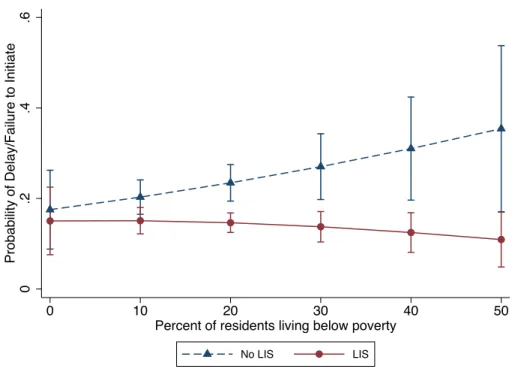
Figure 4. Probability of Treatment Delay or Omissions for LIS and Non-LIS Participants at Differing Levels of Census Tract Poverty... 34
Figure 5. Sample Inclusion ... 35
Figure 6. Example CART Tree... 39
Figure 7. Importance Predictors from Tuned Random Forest Algorithm ... 40
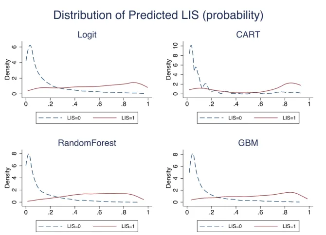
Figure 8. Predicted Probability of LIS Participation by Observed LIS ... 41
Figure 9. Density of Propensity Weights, by Specification ... 42
Figure 10. Cohort Selection ... 64
Figure 11. Adjusted Survival Curves, All-cause and Cancer Specific Mortality, by Medication Delay/Omission ... 69
Figure 12. Adjusted Hazard Ratio Delay/Omission vs. No Delay/Omission, by Cancer Site ... 70
Figure 13. Graph of GBM-generated Predictions, by Delay/Omission status ... 74
Figure 14. Graphical Representation of Simulation Model ... 92
Figure 15. Efficiency Frontier ... 95
Figure 16. Probabilistic Sensitivity Analyses ... 97
Figure 17. Base-case Predicted Probability of Financial Burden, by Disease State ... 99
Figure 18. A Graphical Depiction of Effectiveness Sensitivity Assumptions ... 100
LIST OF ABBREVIATIONS
ACS American Community Survey ATE Average treatment effect
ATT Average treatment effect on the treated
BC Breast cancer
CAHPS Consumer Assessment of Healthcare Providers and Systems CI Confidence interval
FPL Federal Poverty Line
ICER Incremental Cost-Effectiveness Ratio LIS Low-Income Subsidy
ML Machine learning
OOPC Out-of-pocket costs QALY Quality-adjusted life year
EXECUTIVE SUMMARY
Patients navigating a cancer diagnosis and subsequent treatment plan are increasingly likely to list financial burden or financial stress among the many challenging considerations during their care. How this financial burden affects patient decision making, and ultimately outcomes, is not fully understood. In this dissertation, we consider how cancer patients respond to reductions in the cost of prescription medication, the effect of this response on outcomes, and the societal burden associated with negative effects from financial burden in a specific cancer subpopulation. The primary goal of this work is to inform policy decision making related to the cost of care for cancer patients by providing robust, population-based estimates of its
consequences, as well as provide data-informed areas for targeted intervention. To meet these goals, this study is organized into three distinct research aims:
Aim 1: Estimate the protective effect of the low-income subsidy on delay or omission of
prescription medication among Medicare beneficiaries with cancer.
Hypothesis 1: Cancer patients protected from out-of-pocket costs (OOPC) via the low-income subsidy have a lower probability of delay or omission of prescription medication than similar, non-protected patients.
Consumer Assessment of Healthcare Providers and Systems (CAHPS) survey data, we estimated the difference in delay or omission of prescription medication between those on the LIS and not, balancing LIS and non-LIS beneficiaries using machine learning propensity methods.
After achieving good balance on characteristics of LIS and non-LIS groups, we found large and significant reductions in the probability of delay or omission of prescription medication for LIS beneficiaries compared to non-LIS beneficiaries (up to 75%). The result was robust to a number of different specifications and appears to be concentrated in a population weighted to look similar to LIS beneficiaries (i.e., a low-income population), with reduced effectiveness in the full population.
Aim 2: Estimate the effect of financially-motivated delay or omission prescription
medication on mortality among Medicare beneficiaries with cancer.
Hypothesis 2: Cancer patients reporting delay or omission of prescription medication due to cost are at higher risk of all-cause and cancer-specific mortality
Also using the SEER-CAHPS data resource, we estimated the differential hazard of death due to any cause, and due to cancer, associated with a delay or omission of prescription
medication due to cost. Selection into delay/omission is modeled using machine learning techniques and adjusted using propensity analysis, as in Aim 1. Results were presented pooled and stratified across 5 main cancer sites.
Aim 3: Estimate the reduction in benefit (to the individual and to society) associated with
high financial burden for women with early-stage (I/II) HER2+ breast cancer.
Using estimates from Aim 1 and 2 and focusing on HER2+ early stage breast cancer (stage I/II), we estimated the societal loss associated with financial burden attributable to OOPC for prescription drugs using a simulated 10,000 women cohort. Two primary mechanisms of action of financial harm were explored: excess mortality due to quality of life decrements and treatment delay/omission. We compared a setting with no policy intervention on financial burden to hypothetical policies corresponding to sliding scale benefits that offer prescription medication at near zero cost (similar to LIS program) at different levels of income (as percent of the Federal Poverty Line [FPL]).
The simulation demonstrated considerable loss attributable to high OOPC payments for prescription medication; the difference between a setting without any policy intervention and a setting with no financial burden (i.e., probability of burden=0 or all OOPC covered) was
equivalent to more than a full year in perfect health over a 10-year time horizon. Across a range of sensitivity and scenario analyses, we found evidence that a program which substantially reduces the cost of prescription medication (similar to the LIS) for persons at or below 150% FPL, offers a cost-effective societal benefit substantively below conventionally accepted
willingness to pay thresholds. The increased cost associated with shielding the entire population from the cost of prescription medication, however, is likely to be less efficient (more costly and lower marginal benefit) than targeted interventions.
CHAPTER 1: INTRODUCTION
Background
Large improvements in the treatment and management of cancer have changed how we view the disease. While cancer was once a diagnosis with limited evidence-based treatment options, the latter half of the 20th century brought surgical, radiological, and pharmacological
treatment into routine care.1 Coupled with early detection efforts using computed tomography
and other imaging diagnostics, prognosis and quality of life has improved dramatically as a result of technological advancements. Since the late 1990s, a new class of targeted therapies have promised even greater benefit with fewer toxic effects.2 At least one potential side effect of
treatment, however, not commonly measured in clinical trials, threatens to slow years of outcomes-driven progress in cancer care: patient financial burden.
The total cost of cancer has been steadily rising since the 1990s, easily outpacing general and medical price inflation.3,4 Rising costs are distributed throughout the healthcare system, from
private payers, to government, to individual patients.5 Rapidly rising costs are concerning for any
payer, but for individual patients, the effects can be devastating. Early evidence suggests that patients with high financial burden are more likely to file for medical bankruptcy, more likely to be emotionally distressed, and more likely to delay or discontinue treatment.6–9 Indeed, the
debate over high out-of-pocket cost (OOPC) for cancer treatment has made national headlines repeatedly over the last 10 years.
effectiveness of strategies used to reduce it. The vast majority of current evidence addresses the first category, focusing on prevalence and risk factors, though there is some newer evidence related to how burden affects patients (the second). The goal of this study is to add to the limited evidence one second and third categories above – how financial burden affects outcomes and how cancer patients react to reductions in the cost of their care.
Related Literature
The literature on financial burden and cancer health outcomes is relatively small, but growing. We distinguish between studies reporting the specific OOP cost of care from those that attempt to connect high cost with patient outcomes or experience including quality of life, adherence to treatment, or other related cancer outcomes. The latter is the focus of this review, but where important (and especially in early years), we reference more descriptive cost studies, as they can help provide context to the problem.
Literature for this review is gathered using both search strategy (searching within PubMed and Google Scholar) as well as a secondary scan from references of known/identified related sources and systematic reviews. At least two recent systematic reviews (2016, 2017) have been published on financial burden/financial toxicity (discussed below). We focus discussion here to studies conducted within the US.
Much of the early literature on financial burden in cancer focused on describing costs across different populations. Chang and colleagues, noting that many of the existing ‘burden of disease’ estimates came from national surveys, estimated direct medical costs from private insurance claims from 1998-2000.10 Yabroff and colleagues duplicated these findings in
diagnosis, continuing, and last year of life) can have substantially different cost.11 Langa and
co-authors were among the first to focus exclusively on cancer OOP costs for elderly individuals, using data from the 1995 Asset and Health Dynamics Study.12 Unsurprisingly, these authors
found substantial OOP cost for patients especially in the area of prescription medications (data prior to Part D benefit plans). Not long after, cancer site specific OOP cost estimates began to emerge, starting with common sites such as prostate and breast cancers.13,14 In one of the first
studies linking what a patient might pay for cancer treatment to outcomes such as receipt of care, screening and survival, Ward and colleagues used data from the National Health Interview Survey (NHIS) from 1991 to 2004 to estimate differences in outcomes by insurance status among cancer patients. The authors presented their findings acknowledging heavy limitations in the complex relationship between insurance health outcomes.7
With the introduction of Part D in 2006, the realized cost to Medicare beneficiaries for prescription drugs changed dramatically. Knowledge about the program and its costs were limited, especially in early years. One (non-cancer specific) study demonstrated a substantial knowledge gap for patients, as well as more than a quarter who reported cost-coping strategies even after they secured coverage.15 The American Society For Clinical Oncology (ASCO) issued
national guidance on the cost of cancer care in 2009 as a response to increased interest, and to policy changes such as Part D coverage.16 This guidance included recommendations to discuss
cost as an important component of cancer care, to educate patients and physicians, and to fund research to help the cancer community understand factors associated with cost burden.17
a patient convenience sample survey to understand the impact of the cost of cancer treatment on outcomes. Overall they found that almost 40% of patients with household incomes less than $40,000 report a “large amount of distress” as a result of cancer treatment bills.24 Hofstatter
(2010) found virtually no evidence on patient-communication about cost prior to 2009.25
Henrikson and colleagues sought to correct the lack of evidence with a 2014 qualitative study around patient-physician communication and costs in cancer. They found willingness on both sides to discuss costs, but a significant barrier in access to reliable and patient-specific
estimates.26 In a 2012 study, a group of authors described risk factors associated with financial
toxicity in colon cancer patients, including total income and stage of diagnosis. Similar to other studies they found a significant proportion of patients on elected treatment experience financial hardship (38%).27 Describing an important link between treatment discontinuation and high
financial burden, Kasiaeng and colleagues used Medicare claims data to estimate up to 20% increase in the likelihood of discontinuation for patients with higher cost burden.9 Neuner used
the low-income subsidy program to identify differences in adherence for aromatase inhibitors.17
In a large multi-period pilot study using a convenience sample of insured diagnosed cancer patients, Zafar and colleagues found a wide range of financially induced disruptions to daily living and optimal care. Patients cut back on leisure activities (68%), reduced spending in other areas (46%), used less than the prescribed amount of medication (20%), partially filled prescriptions (19%), and avoiding filling prescriptions altogether (24%).6 Researchers have also
attempted to estimate changes in patient decision making as a result of high financial burden. Wong and colleagues (2013) and Fung and colleagues (2013) both looked at tradeoffs and
More recently, researchers have begun to examine how specific subpopulations react to cost burden. Crouch and colleagues studied the difference between rural and urban costs for end of life care for cancer patients.30 Another study suggests that younger rural patients are more
likely to forgo medical care than urban counterparts.31 Wheeler and colleagues found interesting
associations between financial burden and race that were largely attenuated when controlling for socioeconomic status.32 Overall, there appears to be a predictable pattern of increased cost
burden associated with minority or disadvantaged populations.
Lastly, a much smaller number of studies have attempted to link financial burden to hard outcomes, specifically mortality. Tucker-Seeley used the Health and Retirement Study data from 1996-2004 to suggest associations between cost and mortality in older adults (prior to part D and non-cancer specific).33 Using a more rigorous design focused exclusively on cancer patients,
Ramsey and colleagues provided perhaps the strongest evidence to date of an association between financial hardship in cancer and mortality. With Washington state bankruptcy records linked to the Washington SEER Cancer Registry, the authors demonstrated a risk up to 2.65 times greater for patients diagnosed with cancer of filing for bankruptcy, compared to those without cancer.34 In the follow-up study (2016), propensity score matching on cases of
bankruptcy identified in the prior work (vs no bankruptcy – all cancer patients) was used to estimate a relative hazard of death of 1.79 [95% CI: 1.64, 1.96].35
At least two studies reviewed the available evidence on financial burden and financial toxicity in cancer.36,37 The bulk of their findings are discussed above (non-US studies have been
patient-reported instrument surrounding financial burden: the COST measure.38 The measure was
developed in cancer patients and may help to standardize measures across studies, but to date, has few applications. Gordon and colleagues also made note of a specific need for improved evidence on long-term adherence and financial toxicity.
While not providing empirical estimates themselves, it is worth noting that in addition to the estimates provided above, recent years have seen a number of calls to action and
commentating pieces offering insight into patient financial toxicity from multiple
perspectives.8,39–43 Recommendations include longer term policy-oriented solutions, changes in
insurance design and reimbursement, and heightened awareness by physicians and patients.
Significance, Contribution, and Innovation
The cost of cancer care has received considerable public attention over the last 10-15 years.44 More and more, patients, their families, and their providers are recognizing financial
burden itself as an adverse effect of cancer treatment, similar to other treatment ‘toxicities’. Unfortunately, medical care costs are largely unknown at the time of treatment planning, leaving patients confused, or unable to tell if they can afford recommended treatment.6,26
cancer-specific) or progression of disease. The links from financial burden to these hard
endpoints has been largely suggested, but not well tested in a cancer population.39 One important
study looking at all-cause mortality used a single mechanism – bankruptcy – to strengthen the design, but other mechanisms should be explored. No studies that we aware of attempt to associate high financial burden with cancer-specific mortality.
Another large limitation of the existing evidence, and consistent barrier to additional studies, is the large degree of selection into patterns of care. Costs are generally not randomly assigned, and thus differential outcomes observed are difficult to attribute with certainty to the burden of cost itself, and not to other correlated disease or social factors. Robust study designs and statistical methods are needed to test findings under different assumptions, with attempts to control for selection into ‘treatment’ (i.e., high cost).
Finally, virtually no information exists about the impact financial burden may have on greater societal well-being. Cost-effectiveness and economic evaluation in cancer is common and useful for making average treatment decisions based on value derived in the ‘ideal’ setting. These estimates, however, often fail to account for individual ability to pay or other downstream consequences of financial burden. Without the ability to project an expected attributable societal loss due to cost burden, it is difficult to determine the level and target of appropriate intervention. In general, the impact of financial burden on societal benefit has not been quantified. Additional work is needed to understand if these consequences can alter societal-level decision making either in specific subgroups, or even on a population as a whole.
services cancer care. In cancer, estimates of the cost of care have traditionally faced a tradeoff between a large sample, rich disease-focused data source (e.g., registry data, such as SEER) vs. a smaller sample in a survey with direct questions to patients about cost. In this study, we use a rich linked data source which combines detailed cancer specific information, Medicare claims, and patient-reported survey measures. This data resource is relatively new (available 2016) and provides insights not previously available from single data sources previously.
Another shortcoming in the literature surrounding burden of cost in cancer care is one of selection. It is difficult separate the effect of financial burden on outcomes from individual choice, comorbid illness, or disease severity. Sicker individuals, for example, tend to incur higher cost, and experience worse outcomes. This study, benefiting from the richness and
variability of data sources uses novel data science and machine learning methods to help account for this selection. Machine learning methods are a loose collection of computational algorithms that search for multifaceted relationships in pursuit of high-performance prediction, and are well-suited for settings with complex relationships and potentially large number of covariates
(predictors). The use of these methods is still relatively uncommon, but offers an innovative opportunity to tackle a difficult confounding problem in a different way.
Finally, much of the public conversation about the cost of cancer care skirts around discussions about value. Value is an historically complex and difficult topic in medicine. Still, it plays an important role in policy decision making. This study uses an innovative approach to value assessment and economic evaluation – one which challenges the ‘ability to pay’
Conceptual Model
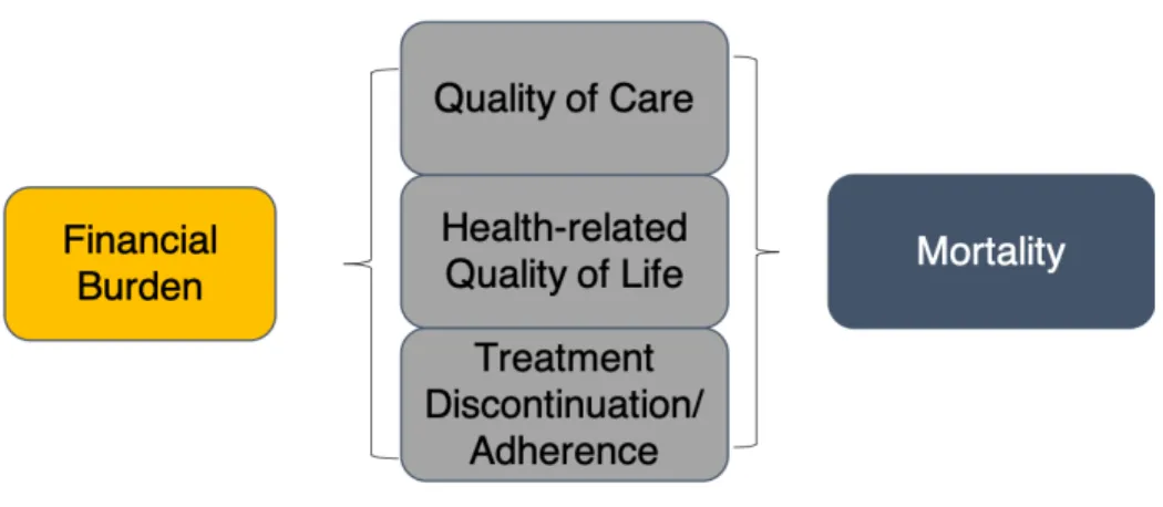
Figure 1 shows a conceptual model adapted from Zafar and colleagues.40 The model
relates high financial burden to cancer health outcomes and ultimately mortality. More
specifically, the model hypothesizes a direct relationship between high financial burden and a patient’s treatment-related choices (discontinuation, delay, decision to take or omit treatment altogether), health-related quality of life, and quality of care. Financial burden has a relationship to mortality and recurrence or disease progression through the mediating factors. Aim 1 of this study focuses specifically on the effect of the LIS program, which reduces OOPC for
prescription drugs on treatment-related outcomes. Aim 2 provides an empirical estimate of the relationship between financially-motivated delay of prescription medication and mortality. Aim 3 combines all aspects of the conceptual model into simulation of the impact to society from high financial burden to individuals using a specific cancer setting (HER2+ breast cancer) as a case study.
Objective Statement
Figure 1. Conceptual Model
CHAPTER 2: HIGH COST BURDEN AND DELAY OR OMISSION OF PRESCRIPTION MEDICATION: A MACHINE LEARNING APPLICATION
Overview
Background: The cost of care remains a significant barrier to guideline-recommended treatment in cancer, as well as a significant burden to patients and their families. Population-based estimates are needed to estimate the effects of out-of-pocket cost protection on medication delays or omission.
Objective: To estimate the effect of out-of-pocket cost protection for prescription medication, proxied by the joint Medicare/Medicaid Low-Income Subsidy (LIS) program, on delay or failure to initiate prescription medication for Medicare beneficiaries with cancer (lung, breast, prostate, bladder, or colorectal).
Methods: We use a three-way link between SEER cancer registry, Medicare claims, and Consumer Assessment of Healthcare Providers and Systems survey to estimate average
treatment effects (ATE) and average effects of treatment among the treated (ATT) of LIS. Using machine-learning algorithms we first predict low-cost exposure, via the LIS, as a function of, cancer-specific characteristics, and diagnosis codes from claims. Applying stabilized propensity weights to adjust for observed differences between LIS and non-LIS participants, we predict self-reported differential risk of delay or omission of prescribed medication.
learning algorithms balance covariates well (mean standardized difference 5-7%). For LIS compared to non-LIS participants, medication omission or delay was -8.3 [95% CI: -11.6, -5.0] percentage points lower in the ATT estimates, and -3.5 [-6.1, -0.1] lower in the ATE estimates in preferred models. Results were similar across a range of specifications and sensitivity analyses but varied considerably by cancer site; breast and colorectal patients had the largest average reduction in medication delay or omission as a result of lower cost burden.
Conclusions: Out-of-pocket cost protection offered by the LIS may significantly reduce the likelihood of omission or delays to prescription medication for Medicare beneficiaries with cancer. Results are concentrated among the most vulnerable and needy.
Introduction
Coupled with early detection efforts, surgical, radiological, and pharmacological treatment have dramatically altered prognosis and quality of life for patients with cancer in the last 50 years.1 At least one potential side effect of treatment not commonly measured in clinical
trials, however, threatens to slow years of outcomes-driven progress: patient financial burden. In recent years, conversations focused on the ‘financial toxicity’ of cancer care have made the cancer community more aware of the toll financial burden can have on cancer patients and cancer survivors.8,45 Early work has demonstrated an association between financial burden and
quality of life, discontinuation of treatment, and mortality.9,46,47
effect of financial burden on outcomes, both intermediate (e.g., failure to receive or delay treatment) and long-term (e.g., disease progression/mortality), is sparse.
Confounding also currently plagues the financial burden literature. It is difficult to separate the effect of financial strain on outcomes from competing clinical or social risk factors often associated with worse outcomes.49 The problem does not lack for data, however. Claims,
registry, and survey data are robust in cancer populations. An environment with complex inter-dependent relationships and rich data is ripe for machine learning (ML) methods, a loose collection of computational algorithms that search for multifaceted relationships in pursuit of high-performance prediction.
This study focuses on the intermediate outcome of access to prescription medication, an important marker for long-term outcomes in cancer care.50 Though not the only barrier to access,
cost and financial considerations are frequently reported by patients as prohibitive to recommended treatment.51,52 We examined the differential impact of cost exposure on
medication delay or omission in patients with cancer, applying ML methods to balance between exposed and unexposed groups. We used low-income subsidy (LIS) participation – a proxy for significant protections against high-cost prescription medication – as our primary exposure. In a propensity balanced sample, we tested whether cancer patients with LIS, and accordingly lower cost burden, were less likely to delay or fail to initiate prescribed medication.
Methods
differences in selection into the LIS program using the potential outcomes framework and ML-generated propensity scores.
Data
Data for this study come from a unique three-way linkage of the Surveillance, Epidemiology, and End Results Program (SEER) Cancer registry53, fee-for-service (FFS)
Medicare claims, and the Consumer Assessment of Healthcare Providers and Systems (CAHPS) survey.54 The linkage contains a rich set of demographic, clinical, and utilization-based
covariates often lacking from survey, claims, or registry data alone. We included data from all three sources from 2007-2015 (with claims dating back to 2002). In addition, we merged area-level socio-demographic and poverty measures from the American Community Survey (ACS) at the Census Tract level.
Cancer Sample
Outcome
The primary outcome of interest was a self-reported measure of delay or failure to fill prescription, a binary response to the query: “In the last 6 months, did you ever delay or not fill a prescription because you felt that you could not afford it?” The wording helps define a short time window that improves confidence in the co-occurrence of our outcome and exposure. The
question also focuses on delays made exclusive to cost-specific barriers, eliminating the need to separate delay or omission of prescription medication not attributable to cost. This outcome measure was available for all survey years 2007-2015.
Exposure
We used as our primary exposure, LIS enrollment - a proxy for significant protections against high-cost prescription medication. The LIS is a joint Medicare-Medicaid administered program intended to offer prescription medication to needy individuals at zero or near-zero cost. Eligibility pertains to 150% of the Federal Income Poverty Level (FPL) and below, subject to additional minimum asset requirements. Since the LIS is a Part D (prescription drug benefit) program, we restricted our primary sample to Part D beneficiaries. The LIS was determined by the Medicare enrollment file (i.e., not a self-reported measure).
Covariates
classified diagnoses, up to five years prior to survey completion. The ICD-9 codes were categorized into 285 clinical classifications using the AHRQ Clinical Classification Software (CCS) for comorbidity.55,56 Area-level measures of percent black, white, and Hispanic ethnicity,
as well as educational attainment, median income, population density, and the percent of individuals living below poverty were included at the Census Tract level.
Design and Analysis
Because we expected a considerable amount of selection into exposure, we attempted to balance treated (LIS=1) and control (LIS=0) groups using the potential outcomes framework developed by Rubin and inverse probability of treatment weighting (IPTW).57 How we applied
weights determined the specific counterfactual being estimated: the average treatment effect on the treated (ATT), or the average treatment effect (ATE).57,58 In this setting, the ATT, which
focuses on effects among those most likely to receive the LIS, may be more appropriate than the ATE, which estimates effects in the full population.
To estimate the desired potential outcomes, we first attempted to flexibly account for differences in treatment assignment. We used ML methods that apply a ‘learning’ algorithm to prediction, allow a large number of predictors (e.g., interaction and higher order terms), and rely less on functional form.59–62 We tested three popular ML algorithms, each of which, in their
simplest form, split observations into high-dimensional, mutually exclusive groups to generate predictions (referred to as ‘trees’): Classification And Regression Trees (CART), Random
used a 5-fold cross-validation out-of-bag sampling procedure to tune ML models.64 Area under
the receiver operating curve (AUC) and Cohen’s kappa were used as performance metrics (tuning details provided in Supplement B). All machine learning models included as predictors all available covariates, including the full list of 285 diagnosis codes from the CCS, coded as 1 if captured in the last five years, and 0 otherwise.
Tuned ML algorithms produced a predicted probability of treatment for the LIS and prescription insurance exposures, respectively. These probabilities were converted to a propensity weight according to the specific effect estimate of interest (ATT or ATE), and ‘stabilized’ to reduce variance.65 For comparison, we also estimated models with propensity
scores built from a logistic regression first stage model on a limited set of covariates (no
interactions and without the full CCI claims codes). Graphically, we demonstrate the reduction in standardized difference (𝑥̅#$%&#'%(#− 𝑥̅*+(#$+,/𝜎/) across a range of selected covariates to
demonstrate suitable balance. Outcome models were estimated using weighted logistic regression that also controlled for socio-demographic and cancer-specific covariates (doubly robust). Treatment effects were presented as marginal effects (risk differences) for each of the three different ML algorithm-generated propensity scores. We conducted sensitivity analyses to demonstrate the robustness of our results across missing data specifications, including ML selection of missing category, complete case, and multiple imputation.66 Analyses were
conducted using R v3.5.1 and Stata 15.
Subgroup and Sensitivity Analyses
recommendations for different sites, we expect our effects may be heterogenous as well. Second, we restricted the sample to individuals with a cancer diagnosis within two years of survey
response to mimic a “newly-diagnosed” cohort. Third, we limited the sample to individuals living in the lower 50th percentile of Census Tract poverty status observed in our data (~11% of
FPL). This approach creates a more homogenous sample which may improve balance.
Results
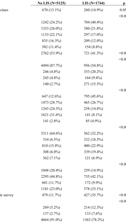
The primary sample included 6,869 cancer patients diagnosed between 2007 and 2015 (Supplement A). Unweighted, approximately 34% participated in the LIS at the time of survey and nearly 14% overall report having delayed or failed to initiate a prescription medication in the six months preceding their survey response (Table 1). LIS participants were approximately two percentage points more likely to delay or omit prescription medication than those not on the LIS. LIS participants were also less likely to have a college education, more likely to be minority race, and considerably less likely to be married.
ML algorithms predict LIS status using covariates from Table 1 as well as individual CCS codes from claims. In general, both Random Forest and GBM algorithms predict LIS status well, with race, education, and marital status were among the strongest predictors of LIS status. Additional fit statistics, propensity distributions, and details for ML algorithms are found in Supplement B-C. Though not a guarantee of bias reduction59, weighted standardized differences
between LIS and non-LIS participants were reduced from up to 80% in some cases to below 10% on average in all model specifications (Figure 2).
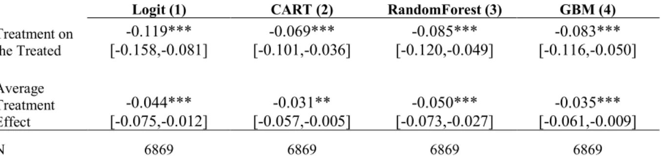
presented in supplemental materials [Table 5]). Overall, after balancing, the LIS was shown to be protective against medication delay or omission. The primary ATT effect (i.e., within a
population weighted to look similar to LIS participants) was strongly negative, statistically different from zero at the 1% level, and similar across all propensity specifications (GBM: -8.4 [95%CI: -12.0, -4.7]). ATE estimates (i.e., within a population weighted to look like the full sample) were also similar across specifications, negative, and statistically different from zero, but attenuated compared to ATT estimates.
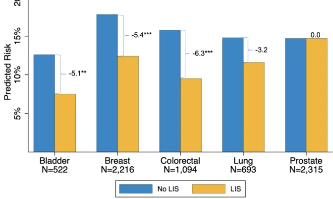
Figure 3confirms considerable heterogeneity by site, with strong negative and significant effects for breast and colorectal cancers and negative but smaller associations and larger standard errors for bladder and lung (with smaller samples). Prostate cancer was the only non-negative ATE.
Additional sensitivity analyses
Restricting the sample to patients diagnosed with cancer within 2 years of their survey date (“newly diagnosed”) produced very similar estimates to the main findings (Table 3, Model 1). Similarly, alternative missing data specifications, complete case analysis and logit-propensity multiple imputation, all were consistent (Table 3, Models 2-3).
poverty levels, risk of delay/omission was substantially increased for non-LIS individuals living in the most vulnerable areas.
Discussion
Financial burden may be a significant barrier to guideline recommended care for some cancer patients. In this study, we use the Low-Income Subsidy program, intended to eliminate or drastically reduce the cost of prescription drugs, as a measure of reduced medication cost burden to individuals. Because the program is available only to low-income individuals who may otherwise receive less than optimal care, we employ a machine-learning propensity-adjusted approach to effect estimation.
In general, we find large and significant reductions in the likelihood of delay or omission of medication for those protected by the LIS. Depending on the specific estimator used,
differences range from four to ten percentage points, or a 22-75% in reduction medication delay or omission relative to the baseline likelihood (13.5%). Our findings are robust to a number of different specifications and sensitivity results, different ML algorithms to predict treatment, and alternative approaches to missing data. We presented both ATE and ATT estimates to
demonstrate how effects may vary across selected (LIS) and full populations. In our primary models, ATT estimates were 2-3 times larger than ATE estimates, suggesting a potentially low likelihood of benefit for those not eligible to receive the LIS – an arguably less needy group at baseline based on LIS income and asset eligibility thresholds.
uncontrolled. But the ability to make use of information from many covariates, interactions, and higher order terms systematically, and divorced from instigator biases, is appealing. Importantly, some have cautioned the research community when using ML approaches for causal
inference.62,63 Our approach in this study separates prediction from inference. The goal of the
propensity score with or without ML techniques is to use accurate prediction to balance treated and control groups. Such a task is well-suited for supervised ML techniques like those used here.
We include a number of policy-relevant sensitivity analyses in our study. First, we considered heterogenous treatment effects by cancer site. Substantial variation in effect by cancer site is consistent with the proposed mechanism of action for the LIS. In particular, we highlight the case of prostate cancer, an area where the vast majority of diagnosed patients are under no recommended guidelines that include pharmacologic treatment, and where we observe no average treatment effect. Contrast this to breast cancer, where clinical recommendations include sometimes expensive hormonal endocrine therapy.67 Here we observed consistent
negative ATE and ATT differences – reductions between 5 and 10 percentage points. We also find that those living in poor census tract areas appear to experience a larger benefit to prescription medication cost protection (more than 60% larger ATE than the full sample estimates). This finding is consistent with our expectation that higher income individuals are likely to benefit less from programs that reduce cost. Differential access to care contributes to cancer care disparities and lessens the population impact of technology advancement.68 We are
careful to note that ‘burden’ as defined in the financial toxicity literature takes many forms and affects individuals across levels of socioeconomic status and generosity of insurance
This work contributes to a growing literature on costs and financial burden in cancer care. Kaisaeng and colleagues used Medicare claims to estimate discontinuation of chemotherapy among patients who initiated treatment.9 Consistent with our findings, they observed that
discontinuation may be 20% higher for patients who experience larger costs, but they are limited by what they can see from the material patient burden in FFS Medicare claims. A number of studies have used NHIS survey data to report ‘forgoing medical care’ due to cost in 10-30% of the cancer population.31,51,71 Similarly, in a pilot study of 254 cancer patients, Zafar and
colleagues reported significant patient response to cost burden, including 20% who took less than the prescribed amount of medication, 19% who partially filled prescriptions, and 24% who avoided filling prescriptions altogether.6 Our findings are consistent with these studies, but
extend this work by estimating differences across treated and control groups. A considerable amount of research has focused on the psychological or quality of life burden associated with high cost burden,69,72 an aspect that may be substantially intertwined with the estimated treatment
response.
This work contains a number of limitations. First, we are unable to account for unobserved factors that may confound our primary estimate. Health literacy, trust in the
not be specific to cancer drugs. Even so, we see non-cancer drug response as itself a potentially interesting finding. If patients are prioritizing cancer treatment yet delaying diabetes medication, this can also contribute negative health consequences. Finally, we were not able to standardize our measure of ‘delay.’ A self-reported measure is important, but is difficult to quantify in terms of potential for harm without further investigation.
A number of active and conceived policies and practices seek to curb patient individual cost burden. The hotly debated practice of pharmaceutical couponing (not available to Medicare beneficiaries) offers a similar benefit.73 Many individual states cap the out-of-pocket cost
charges for private insurance plans or require ‘parity’ in coverage between infused and oral medications – provisions that often target the cancer community specifically.74 Our research
supports the notion that these programs are likely to be effective in protecting access for some individuals. In addition, although we are unable to make direct statements about costs not attributable to prescription medication, it is not inconceivable that patients could react similarly to treatment covered by other benefits, such as surgery, radiation, or oncology visits. Without supplemental insurance, original Medicare covers 80% of costs, leaving a large portion
unaccounted for. Nationally, prescription drugs make up less than 15% of total healthcare costs, and though drugs make easy targets, patients face financial burden across the spectrum of healthcare services.75 Not considered here, is the cost of such programs to society. These
Conclusion
Increased cost exposure to prescription medication among Medicare beneficiaries with cancer may lead to delay or failure to initiate treatment. Such effects are likely to be
Tables and Figures
Table 1. Selected Sample Descriptive Statistics (unweighted)
No LIS (N=5125) LIS (N=1744) p
Delay filling prescribed medicines 670 (13.1%) 260 (14.9%) 0.053
Age Category <0.001
<69 1242 (24.2%) 704 (40.4%)
70-74 1333 (26.0%) 380 (21.8%)
75-79 1133 (22.1%) 297 (17.0%)
80-84 835 (16.3%) 209 (12.0%)
85+ 582 (11.4%) 154 (8.8%)
Male Gender 2762 (53.9%) 721 (41.3%) <0.001
Race <0.001
White 4494 (87.7%) 956 (54.8%)
Black 246 (4.8%) 353 (20.2%)
Other 245 (4.8%) 164 (9.4%)
Hispanic 140 (2.7%) 271 (15.5%)
Education <0.001
Some HS, no grad 647 (12.6%) 795 (45.6%)
HS grad 1473 (28.7%) 465 (26.7%)
Some college 1243 (24.3%) 258 (14.8%)
College+ 1621 (31.6%) 141 (8.1%)
Missing 141 (2.8%) 85 (4.9%)
Marital Status <0.001
Married 3311 (64.6%) 562 (32.2%)
Sep/Divorce 334 (6.5%) 322 (18.5%)
Widowed 810 (15.8%) 400 (22.9%)
Never Married 308 (6.0%) 339 (19.4%)
Missing 362 (7.1%) 121 (6.9%)
Region <0.001
Northeast 1048 (20.4%) 259 (14.9%)
West 2295 (44.8%) 735 (42.1%)
Midwest 601 (11.7%) 172 (9.9%)
South 1181 (23.0%) 578 (33.1%)
Someone helped you complete survey 479 (11.7%) 427 (35.7%) <0.001
Smoking Status <0.001
Every day 269 (5.2%) 214 (12.3%)
Some Days 137 (2.7%) 133 (7.6%)
Missing 55 (1.1%) 34 (1.9%)
Urban/Rural <0.001
Metro 4145 (80.9%) 1357 (77.8%)
High Urban 375 (7.3%) 103 (5.9%)
Low Urban 502 (9.8%) 214 (12.3%)
Rural 103 (2.0%) 70 (4.0%)
Cancer Site at Diagnosis <0.001
Bladder 444 (8.7%) 108 (6.2%)
Breast 1596 (31.1%) 619 (35.5%)
Colorectal 755 (14.7%) 339 (19.4%)
Lung 474 (9.2%) 219 (12.6%)
Prostate 1856 (36.2%) 459 (26.3%)
Cancer Stage at Diagnosis 0.015
In Situ (Stage 0) 636 (12.4%) 215 (12.3%)
Stage I 1680 (32.8%) 549 (31.5%)
Stage II 1996 (38.9%) 632 (36.2%)
Stage III 501 (9.8%) 201 (11.5%)
Stage IV 228 (4.4%) 102 (5.8%)
Missing 84 (1.6%) 45 (2.6%)
Cancer Grade at Diagnosis 0.37
Grade 1 590 (11.5%) 186 (10.7%)
Grade 2 2269 (44.3%) 720 (41.3%)
Grade 3 1556 (30.4%) 545 (31.3%)
Grade 4 156 (3.0%) 45 (2.6%)
Missing 554 (10.8%) 248 (14.2%)
Surgery on Primary Tumor 3606 (70.8%) 1238 (71.7%) 0.48
Radiation on Primary Tumor 1833 (35.8%) 594 (34.1%) 0.20
Comorbidities, mean (SD) 6.3 (3.6) 7.9 (3.9) <0.001
Census Tract Covariates
Median Income, mean (SD) 67664.5 (28219.0) 52226.3 (22256.4) <0.001
Density, mean (SD) 3377.7 (4741.1) 4761.2 (8074.1) <0.001
Pct Whites, mean (SD) 76.1 (21.1) 67.9 (24.4) <0.001
Pct Blacks, mean (SD) 8.9 (15.3) 15.8 (22.6) <0.001
Pct Hispanics, mean (SD) 12.1 (14.1) 18.9 (21.6) <0.001
Pct Non-HS Grads, mean (SD) 11.8 (8.1) 18.8 (11.0) <0.001
Pct HS Only, mean (SD) 26.4 (10.2) 29.3 (9.3) <0.001
Pct Some College, mean (SD) 29.6 (7.3) 28.6 (6.9) <0.001
Pct College, mean (SD) 32.2 (16.9) 23.4 (14.6) <0.001
Pct below poverty, mean (SD) 11.9 (8.2) 18.4 (11.3) <0.001
Figure 2. Standardized Differences (LIS vs. No LIS) for Selected Covariates by Propensity Weight
*LIS=low-income subsidy; GBM=gradient booted machine; CART=classification and regression trees. The standardized difference is the [weighted] mean in the treated (LIS) minus the mean in the untreated groups divided by the pool standard deviation, for each covariate listed.
agecat:<69 agecat:70−74 agecat:75−79 agecat:80−84 agecat:85+ Male Gender education:Some HS, no grad education:HS grad education:Some college education:College+ education:Missing race:White race:Black race:Other race:Hispanic maritaldx:Married maritaldx:Sep/Divorce maritaldx:Widowed maritaldx:Never Married maritaldx:Missing urbrur:Metro urbrur:High Urban urbrur:Low Urban urbrur:Rural smokenow:Every day smokenow:Some Days smokenow:Not at all smokenow:Missing proxy:No Proxy proxy:Proxy proxy:Missing cancer:Bladder cancer:Breast cancer:Colorectal cancer:Lung cancer:Prostate cancer:Other stage:In Situ (Stage 0) stage:Stage I stage:Stage II stage:Stage III stage:Stage IV stage:Missing grade:Grade 1 grade:Grade 2 grade:Grade 3 grade:Grade 4 grade:Other(Mostly Lymphoma) grade:Missing Surgery on Primary Tumor Radiation on Primary Tumor Sum of comorbidities Census Tract Median Income Census Tract Density Census Tract Pct Whites Census Tract Pct Blacks Census Tract Pct Hispanics Pct HS only (Tract) Pct College Educ (Tract) Pct below poverty (Tract)
0 .2 .4 .6 .8
Standardized Difference
Table 2. Propensity Adjusted Predicted Difference in Medication Delay or Omission between LIS and Non-LIS participants
Logit (1) CART (2) RandomForest (3) GBM (4)
Treatment on the Treated
-0.119*** [-0.158,-0.081]
-0.069*** [-0.101,-0.036]
-0.085*** [-0.120,-0.049]
-0.083*** [-0.116,-0.050]
Average Treatment Effect
-0.044*** [-0.075,-0.012]
-0.031** [-0.057,-0.005]
-0.050*** [-0.073,-0.027]
-0.035*** [-0.061,-0.009]
N 6869 6869 6869 6869
*Statistically significant at p= **0.05, ***0.001
LIS=low-income subsidy; GBM=gradient booted machine; CART=classification and regression trees.
Figure 3. Heterogenous ATE Effects by Cancer Site
*Statistically significant at p= **0.05, ***0.001
Table 3.Secondary and Sensitivity Analyses
Newly Diagnosed
(1) Complete Case (2) Logit MI (3) Lower 50% Poverty (4)
Treatment on the
Treated [-0.124,-0.041] -0.083*** [-0.124,-0.045] -0.084*** [-0.144, -0.06] -0.102*** [-0.141,-0.056] -0.099***
Average
Treatment Effect [-0.062,0.010] -0.026 [-0.061,0.004] -0.028* [-0.066, 0.003] -0.032* [-0.097,-0.028] -0.063***
N 4621 5993 6869 3498
*Statistically significant at p= **0.05, ***0.001
LIS=low-income subsidy; MI=multiple imputation. Estimates are presented as predicted risk differences calculated from the differential effect of LIS vs. No LIS from gradient boosted machine propensity adjusted logistic regression models using method of recycled predictions and delta method standard errors. Treatment on the treated estimates weight untreated individuals to represent the counterfactual for treated individuals and represent the effect of treatment for those participating in the LIS. Average treatment effect estimates weight treated and untreated individuals by their inverse probability of treatment and represent the effect of treatment on the full sample. Newly diagnosed includes individuals diagnosed within 2 years of survey date. Lower 50% poverty includes individuals living in a census tract with greater than 11% of the population at or below the federal poverty line. Insurance pay is a secondary exposure indicating any insurance coverage to pay for all or part of prescription medications.
Figure 4. Probability of Treatment Delay or Omissions for LIS and Non-LIS Participants at Differing Levels of Census Tract Poverty
LIS=low-income subsidy; Estimates are presented as the predicted risk of medication delay or omission for LIS vs. No LIS from gradient boosted machine propensity adjusted logistic regression models using method of recycled predictions and delta method standard errors. Poverty is defined as the federal poverty line.
0
.2
.4
.6
Probability of Delay/Failure to Initiate
0 10 20 30 40 50
Percent of residents living below poverty
Supplemental Materials
Figure 5. Sample Inclusion
Supplement B: Machine Learning Methods Description
ML algorithms are sensitive to ‘tuning’ parameters – parameters that set specific rules for classification, such as the number of interactions or observations in a group. For example, to avoid small sample or outlier influence, the analyst may specify the minimum number of observations in a final grouping (terminal node) before the algorithm will attempt to ‘split’ or divide further. One systematic tuning technique is cross-validation, which splits data into ‘training’ and ‘testing’ portions (folds) and re-estimates the algorithm over a range of tuning parameters, storing a specific metric or goodness of fit measure (which is produced on the ‘out of bag’ or held-out portion of the sample). The procedure is repeated over each fold, and then re-sampled in its entirety to produce average effects. For final model assessment, it is also common to withhold a portion of the data entirely. This helps to protect against over-fitting of the
algorithm and provide valid accuracy fit statistics. We complete 5-fold cross validation on a 75% random sample of our data, withholding 25% for out-of-bag model assessment. Tuning
Table 4. Selected ML Tuning parameters and Fit Metrics
Model parameter Learning Final node Obs in Covarates Sampled of Trees Number Interactions Maximum Accuracy Kappa
CART 0.001 35 NA NA NA 0.774 0.399
CART 0.005 35 NA NA NA 0.802 0.447
CART 0.01 35 NA NA NA 0.807 0.445
CART 0.015 35 NA NA NA 0.807 0.443
CART 0.02 35 NA NA NA 0.805 0.425
CART 0.025 35 NA NA NA 0.801 0.389
CART 0.03 35 NA NA NA 0.8 0.383
CART 0.001 40 NA NA NA 0.775 0.401
CART 0.005 40 NA NA NA 0.802 0.448
CART 0.006 40 NA NA NA 0.805 0.455
CART 0.007 40 NA NA NA 0.807 0.459
CART 0.008 40 NA NA NA 0.807 0.46
CART 0.009 40 NA NA NA 0.81 0.462
CART 0.01 40 NA NA NA 0.811 0.46
CART 0.015 40 NA NA NA 0.811 0.459
CART 0.02 40 NA NA NA 0.805 0.418
CART 0.025 40 NA NA NA 0.802 0.393
CART 0.03 40 NA NA NA 0.801 0.384
CART 0.001 45 NA NA NA 0.78 0.412
CART 0.005 45 NA NA NA 0.8 0.443
CART 0.01 45 NA NA NA 0.806 0.444
CART 0.015 45 NA NA NA 0.806 0.439
CART 0.02 45 NA NA NA 0.804 0.419
CART 0.025 45 NA NA NA 0.801 0.392
CART 0.03 45 NA NA NA 0.8 0.382
RF NA NA 80 100 NA 0.822 0.485
RF NA NA 100 100 NA 0.821 0.485
RF NA NA 120 100 NA 0.82 0.485
RF NA NA 140 100 NA 0.819 0.482
RF NA NA 160 100 NA 0.818 0.482
RF NA NA 80 250 NA 0.823 0.489
RF NA NA 100 250 NA 0.822 0.489
RF NA NA 120 250 NA 0.823 0.493
RF NA NA 140 250 NA 0.823 0.491
RF NA NA 160 250 NA 0.82 0.487
RF NA NA 80 500 NA 0.825 0.494
RF NA NA 85 500 NA 0.825 0.495
RF NA NA 90 500 NA 0.824 0.494
RF NA NA 95 500 NA 0.823 0.49
RF NA NA 100 500 NA 0.824 0.494
RF NA NA 120 500 NA 0.822 0.49
RF NA NA 140 500 NA 0.823 0.494
RF NA NA 160 500 NA 0.822 0.492
GBM 0.005 35 NA 8000 5 0.832 0.538
GBM 0.005 40 NA 8000 5 0.833 0.541
GBM 0.01 30 NA 8000 5 0.831 0.534
GBM 0.01 35 NA 8000 5 0.83 0.533
GBM 0.01 40 NA 8000 5 0.831 0.535
GBM 0.05 30 NA 8000 5 0.828 0.525
GBM 0.05 35 NA 8000 5 0.826 0.522
GBM 0.05 40 NA 8000 5 0.827 0.524
GBM 0.1 30 NA 8000 5 0.828 0.525
GBM 0.1 35 NA 8000 5 0.826 0.521
GBM 0.1 40 NA 8000 5 0.824 0.514
GBM 0.5 30 NA 8000 5 0.821 0.514
GBM 0.5 35 NA 8000 5 0.819 0.513
GBM 0.5 40 NA 8000 5 0.818 0.505
GBM 0.005 30 NA 8000 6 0.833 0.541
GBM 0.005 35 NA 8000 6 0.833 0.539
GBM 0.005 40 NA 8000 6 0.832 0.538
GBM 0.01 30 NA 8000 6 0.831 0.533
GBM 0.01 35 NA 8000 6 0.831 0.536
GBM 0.01 40 NA 8000 6 0.831 0.536
GBM 0.05 30 NA 8000 6 0.829 0.527
GBM 0.05 35 NA 8000 6 0.827 0.522
GBM 0.05 40 NA 8000 6 0.828 0.525
GBM 0.1 30 NA 8000 6 0.826 0.519
GBM 0.1 35 NA 8000 6 0.825 0.519
GBM 0.1 40 NA 8000 6 0.827 0.523
GBM 0.5 30 NA 8000 6 0.814 0.501
GBM 0.5 35 NA 8000 6 0.814 0.498
GBM 0.5 40 NA 8000 6 0.816 0.507
*Final models are highlighted in yellow.
**Depth=interaction depth; ntree=number of trees; mtry=number of sampled covariates used; sp=minimum number of observations in terminal node; cp=complexity parameter (minimum deviance for continued split);accuracy=percent of correct responses; roc=area under the receiver operating curve; avgdiff= average standardized difference across covariates
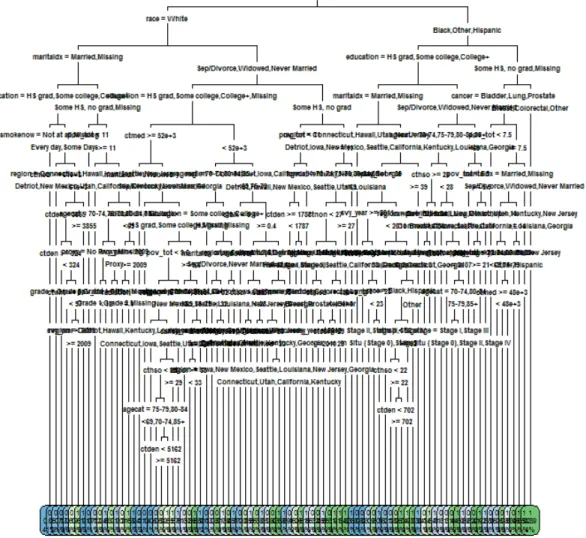
Figure 6. Example CART Tree
This is the final tree created by the CART algorithm. Labels are not intended to be readable, rather the purpose is to show the general structure. Each final node represents a differential probability of selection into the LIS program
Supplement C: Propensity Model Diagnostic Figures
Figure 8. Predicted Probability of LIS Participation by Observed LIS
*LIS= low-income subsidy
0
2
4
6
Density
0 .2 .4 .6 .8 1
LIS=0 LIS=1 Logit 0 2 4 6 8 10 Density
0 .2 .4 .6 .8 1
LIS=0 LIS=1 CART 0 2 4 6 8 Density
0 .2 .4 .6 .8 1
LIS=0 LIS=1 RandomForest 0 2 4 6 8 Density
0 .2 .4 .6 .8 1
LIS=0 LIS=1
GBM
Figure 9. Density of Propensity Weights, by Specification
0
.2
.4
.6
.8
1
Density
0 2 4 6 8 10
Stabilized Propensity Weights
Weights Above 1
0
5
10
15
20
Density
0 .2 .4 .6 .8 1
Stabilized Propensity Weights
Logit CART Forest GBM
Weights Below 1
Supplement D: Primary Model Coefficients
Table 5. Relative Measures (Odds Ratio)
ATE ATT
Odds Ratio 95% CI Odds Ratio 95% CI
Delay or Omission 0.718*** [0.562,0.917] 0.548*** [0.432,0.694]
Breast 1.573** [1.039,2.380] 1.638* [0.960,2.795]
Colorectal 1.302 [0.881,1.926] 1.443 [0.848,2.456]
Lung 1.31 [0.842,2.037] 1.391 [0.782,2.475]
Prostate 1.333 [0.883,2.012] 1.564 [0.886,2.763]
Age
70-74 0.551*** [0.446,0.682] 0.506*** [0.387,0.662]
75-79 0.390*** [0.305,0.500] 0.404*** [0.292,0.558]
80-84 0.339*** [0.254,0.451] 0.369*** [0.257,0.530]
85+ 0.226*** [0.154,0.330] 0.240*** [0.150,0.384]
Male 1.308* [0.976,1.752] 1.343 [0.945,1.909]
Race
Black 1.153 [0.825,1.613] 0.882 [0.643,1.210]
Other 1.587* [0.964,2.613] 1.079 [0.649,1.792]
Hispanic 1.680** [1.115,2.532] 1.248 [0.855,1.822]
Education
HS grad 0.939 [0.732,1.205] 1.175 [0.900,1.534]
Some college 0.984 [0.749,1.291] 1.079 [0.785,1.484]
College+ 0.694** [0.514,0.938] 0.803 [0.544,1.187]
Missing 0.985 [0.604,1.604] 0.779 [0.453,1.340]
Marital Status
Sep/Divorce 1.196 [0.900,1.589] 1.018 [0.749,1.383]
Widowed 1.18 [0.914,1.523] 1.14 [0.842,1.544]
Never Married 0.91 [0.649,1.275] 0.661** [0.465,0.938]
Missing 1.406** [1.010,1.957] 1.38 [0.904,2.109]
Urban Rural
High Urban 0.956 [0.669,1.365] 1.029 [0.668,1.584]
Low Urban 1.091 [0.811,1.468] 1.022 [0.713,1.463]
Rural 0.941 [0.558,1.586] 0.973 [0.539,1.757]
Smoking
Some Days 1.432 [0.897,2.285] 1.466 [0.912,2.358]
Not at all 1.032 [0.742,1.435] 1.129 [0.795,1.604]
Missing 1.826* [0.927,3.596] 1.784 [0.811,3.925]
Missing 1.015 [0.816,1.262] 1.21 [0.954,1.536] Region
West 1.052 [0.774,1.429] 1.179 [0.787,1.769]
Midwest 0.994 [0.703,1.405] 1.059 [0.672,1.670]
South 1.206 [0.891,1.632] 1.386 [0.933,2.059]
Cancer Stage
Stage I 0.848 [0.644,1.116] 0.819 [0.576,1.165]
Stage II 0.801 [0.592,1.083] 0.726* [0.503,1.049]
Stage III 0.747 [0.514,1.087] 0.71 [0.452,1.116]
Stage IV 0.701 [0.443,1.110] 0.778 [0.461,1.313]
Missing 0.542* [0.273,1.073] 0.553 [0.259,1.182]
Surgery 1.094** [1.014,1.179] 1.065 [0.971,1.168]
Radiation 1.17 [0.970,1.410] 1.18 [0.940,1.481]
Cancer Grade
Grade 2 1.187 [0.894,1.575] 1.442* [0.992,2.097]
Grade 3 1.133 [0.832,1.543] 1.514** [1.018,2.251]
Grade 4 1.683** [1.005,2.820] 2.424** [1.231,4.773]
Missing 1.315 [0.922,1.875] 1.551* [0.998,2.410]
Comorbidity Count 1.096*** [1.072,1.122] 1.062*** [1.033,1.091]
Census Tract SES
MedianIncome 1 [1.000,1.000] 1 [1.000,1.000]
PctBlacks 1.015*** [1.004,1.026] 1.016*** [1.004,1.029]
Density 1.000** [1.000,1.000] 1 [1.000,1.000]
PctWhites 1.015*** [1.006,1.024] 1.011** [1.001,1.022]
PctHispanics 0.999 [0.991,1.007] 1.002 [0.993,1.010]
PctHighSchoolOnly 0.987 [0.966,1.008] 0.974* [0.949,1.000]
Table 6. Full Set of Coefficients, Final Outcome Models
Outcome model using Logit IPTW weights
ATE ATT
Low Income Subsidy -0.364 [-1.441,0.713] -0.22 [-1.188,0.748]
Breast 0.455* [-0.025,0.934] 0.760* [-0.082,1.603]
Colorectal 0.382 [-0.090,0.854] 0.836* [-0.055,1.726]
Lung 0.241 [-0.280,0.761] 0.326 [-0.600,1.253]
Prostate 0.133 [-0.351,0.617] 0.661 [-0.263,1.586]
LIS # Breast -0.013 [-1.161,1.136] -0.453 [-1.497,0.591]
LIS # Colorectal -0.146 [-1.372,1.081] -0.717 [-1.837,0.402]
LIS # Lung 0.234 [-1.068,1.536] -0.032 [-1.186,1.122]
LIS # Prostate 0.534 [-0.660,1.729] -0.318 [-1.389,0.753]
Age (Ref=<69)
70-74 -0.578*** [-0.830,-0.327] -0.780*** [-1.113,-0.447]
75-79 -0.884*** [-1.168,-0.599] -0.905*** [-1.298,-0.513]
80-84 -0.965*** [-1.323,-0.606] -1.033*** [-1.455,-0.612]
85+ -1.286*** [-1.715,-0.856] -1.156*** [-1.727,-0.585]
Male 0.263 [-0.087,0.612] 0.192 [-0.230,0.614]
Race (Ref=White)
Black -0.114 [-0.503,0.275] -0.303 [-0.681,0.074]
Other 0.514* [-0.090,1.117] 0.182 [-0.448,0.813]
Hispanic 0.694*** [0.189,1.199] 0.412* [-0.060,0.884]
Education (Ref=<HS)
HS grad 0.007 [-0.299,0.313] 0.227 [-0.103,0.556]
Some college 0.058 [-0.284,0.401] 0.071 [-0.310,0.451]
College+ -0.243 [-0.609,0.123] -0.176 [-0.625,0.273]
Missing 0.1 [-0.439,0.638] 0.025 [-0.529,0.578]
Marital (Ref=Married)
Sep/Divorce 0.366** [0.027,0.706] 0.172 [-0.202,0.545]
Widowed 0.174 [-0.125,0.473] 0.076 [-0.275,0.428]
Never Married -0.172 [-0.587,0.242] -0.467** [-0.889,-0.044]
Missing 0.355* [-0.025,0.736] 0.339 [-0.156,0.833]
Urban/Rural (Ref=Metro)
High Urban -0.268 [-0.669,0.133] -0.228 [-0.744,0.288]
Low Urban 0.1 [-0.291,0.492] -0.021 [-0.474,0.431]
Rural -0.626 [-1.405,0.153] -0.637 [-1.505,0.231]
Smoking (Ref=Most Days)
Some Days 0.151 [-0.417,0.719] 0.215 [-0.356,0.787]
Not at all -0.25 [-0.651,0.151] -0.201 [-0.629,0.227]
Missing 0.239 [-0.510,0.989] 0.118 [-0.774,1.009]
Year of Survey -0.047** [-0.086,-0.008] -0.032 [-0.084,0.021]
Proxy 0.276 [-0.085,0.638] 0.215 [-0.193,0.624]
Missing 0.207 [-0.059,0.472] 0.253* [-0.030,0.537]
West 0.02 [-0.345,0.385] 0.244 [-0.275,0.762]
Midwest 0.189 [-0.241,0.619] 0.164 [-0.370,0.698]
South 0.127 [-0.223,0.476] 0.298 [-0.185,0.781]