U
NDERSTANDINGM
ECHANISMSU
NDERLYING THEL
ONG-
TERME
FFECTSOF
S
CHOLARSHIPS FORS
ECONDARYS
CHOOL: E
VIDENCE FROM AL
ARGEF
IELDE
XPERIMENT INC
OLOMBIAChristian Manuel Posso Su´arez
A dissertation submitted to the faculty of the University of North Carolina at Chapel Hill in par-tial fulfillment of the requirements for the degree of Doctor of Philosophy in the Department of
Economics.
Chapel Hill 2015
Approved by:
David Guilkey
Saraswata Chaudhuri
Klara Peter
Helen Tauchen
c
2015
Christian Manuel Posso Su´arez ALL RIGHTS RESERVED
ABSTRACT
CHRISTIAN MANUEL POSSO SU ´AREZ: Understanding Mechanisms Underlying the Long-term Effects of Scholarships for Secondary School: Evidence from a Large Field
Experiment in Colombia. (Under the direction of David Guilkey)
I examine the long-term effects of educational subsidies programs on adult labor market
out-comes through the accumulation of human capital. Combining experimental variation with an
appropriate econometric model, I present sufficient conditions to identify the long-term effects on
adult outcomes of educational subsidies programs under the presence of unobserved confounders
that affect both the causal mechanism and the adult labor market outcomes. Using a large-scale
program that randomized scholarships for private secondary school among disadvantaged students
in Bogota Colombia in 1994, and Colombias administrative records covering schooling decisions
and labor outcomes up to 15 years after the scholarship lottery, I find causal effect of the program
on wages and labor force participation through the accumulation of human capital is significant
and strong. I also find evidence of dynamic selection on educational attainment and selection on
gains. The results provide important implications for the design of educational programs that target
Without my wife, Ana Maria Lemos, and my daughter, Maria-Jose Posso this project would have
never been started, and would have never been completed. I will always be in debt to you. Thank
You.
ACKNOWLEDGMENTS
I am grateful to my advisor Professor David Guilkey for his continuous guidance, encouragement
and support at every stage of this dissertation. I am also indebted to my dissertation committee
members Saraswata Chaudhuri, Klara Sabirianova Peter, Helen Tauchen, and Tiago Pires for their
invaluable advice and support. I would also like to thank Carlos Medina, Arlen Guarin, Donna
Gilleskie, Brian McManus and participants of the UNC Applied Microeconomics Workshop for
their continue support and helpful comments. It should be noted that this research would not be
possible without the continue support of the Central Bank of Colombia, Banco de la Rep´ublica
de Colombia. The results and conclusions in this dissertation are my own and do not indicate
TABLE OF CONTENTS
LIST OF TABLES . . . viii
LIST OF FIGURES . . . ix
1 INTRODUCTION . . . 1
2 LITERATURE REVIEW . . . 9
2.1 Literature review on long term effects and causal mechanisms . . . 10
2.2 Literature review on the PACES program . . . 15
3 A SIMPLE ECONOMIC MODEL OF EDUCATIONAL ATTAINMENT WITH AN SCHOLARSHIP . . . 19
3.1 The scholarship causal mechanism effect . . . 21
4 FRAMEWORK: A SEQUENTIAL MODEL OF EDUCATIONAL ATTAINTMENT 23 4.1 Factor structure . . . 25
4.2 Identification . . . 26
4.3 Defining Treatment Effects . . . 32
5 ESTIMATION STRATEGY . . . 35
6 DATA . . . 38
6.1 PACES background . . . 38
6.2 Main sample . . . 39
7 RESULTS . . . 46
7.1 Estimated Parameters . . . 46
7.2 Average Treatment Effects of Education on Wages . . . 52
7.3 Policy relevant Treatment Effects . . . 56
7.4 Treatment and Policy Effects on Additional Outcomes . . . 57
A COLOMBIA’S EDUCATIONAL SYSTEM AND PACES BACKGROUND . . . 60
B KOTLARSKI’S THEOREM . . . 61
C SUFFICIENT CONDITIONS FOR IDENTIFICATION OF PARAMETERS AND DISTRIBUTIONS . . . 62
D ALTERNATIVE SET OF ASSUMPTIONS . . . 66
E ADDITIONAL TABLES AND FIGURES . . . 67
LIST OF TABLES
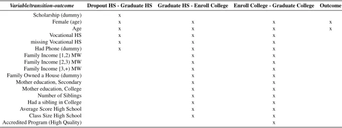
6.1 Observable variables in sequential schooling model and outcomes . . . 43
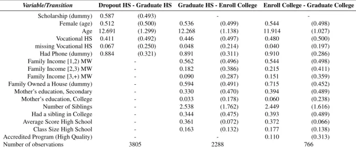
6.2 Sample Statistics: Sequential schooling transitions . . . 44
6.3 Sample Statistics: Outcomes . . . 45
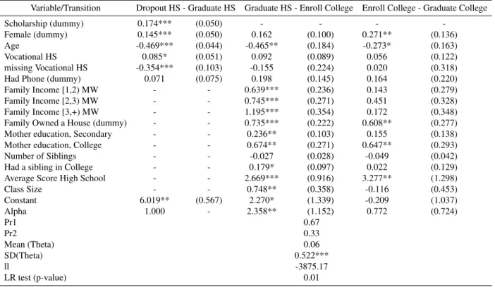
7.1 Estimates for the sequential schooling model . . . 48
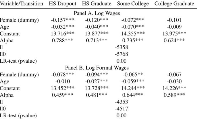
7.2 Estimate coefficients for potential outcomes: wages and formal wages . . . 51
7.3 Treatment Effects for final educational levels: High School dropout as a compari-son group . . . 53
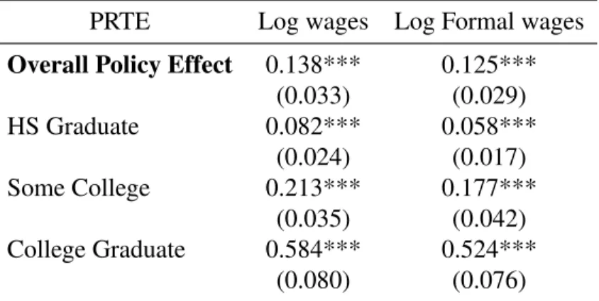
7.4 Policy Relevant Treatment Effects . . . 57
E.1 Variable definitions . . . 68
E.2 Estimates for the sequential schooling model with an additional instrument . . . 69
E.3 Estimates for the sequential schooling model with different distributional assump-tion onθ . . . 70
E.4 Estimates for the sequential schooling model with alternative specification . . . 71
E.5 Goodness of Fit for outcomes . . . 71
E.6 Goodness of Fit for outcomes . . . 72
E.7 Treatment Effects for final educational levels using specification with additional exclusion restrictions: High School dropout as a comparison group . . . 73
E.8 Treatment Effects for final educational levels without unobserved heterogeneity: High School dropout as a comparison group . . . 74
E.9 Estimates coefficients for potential outcomes: Days worked formal market and Sisben score . . . 75
E.10 Treatment Effects (other outcomes) for final educational levels: High School dropout as a comparison group . . . 76
E.11 Policy Relevant Treatment Effects for other outcomes . . . 77
LIST OF FIGURES
1.1 Causal Mechanism of a scholarship program . . . 3
4.1 Sequential Schooling Model . . . 24
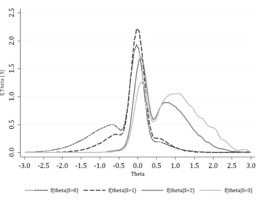
7.1 Densities ofθ by final level of education . . . 50
7.2 Proportion of each decile of0,1 induced to switch by the PACES scholarship . . . 58
E.1 Densities ofPr(D0,1 = 1|scholarship= 1)andPr(D0,1 = 1|scholarship= 0) . . 67
E.2 Observed and simulated percentiles of the log of the monthly wage rate in2010 . . 77
E.3 Observed and simulated percentiles of the log of the monthly formal wage rate in
2010 . . . 78
E.4 Observed and simulated percentiles of Days worked in2010 . . . 78
CHAPTER 1
INTRODUCTION
Recent literature establishes that significant investment in child development at an early age is
one of the key determinants of future adult outcomes. Huggett, Ventura, and Yaron (2011) shows
that for the United States most of the variability in lifetime earnings is explained by personal
attributes determined before age 23.1 Existing studies in labor economics predominantly find that
when these investments are focused on young disadvantaged children, the economic returns are
even higher.2 In particular, there is strong evidence of a positive impact of educational subsidies
and targeted conditional cash transfers on educational outcomes.3 Despite the fact that most of
these policies have the goal of developing human capital in the long run, there has been little
research on long term causal effects on adult outcomes.
This paper estimates the long-term effects of educational subsidies programs on adult labor
market outcomes through the accumulation of human capital. Most of the empirical studies that
evaluate the impact of educational subsidies focus mainly on establishing whether the policy
vari-able impacts a particular outcome, but usually they fail to explain the causal mechanisms through
which the policy affects the outcome.4 This is particularly important in cases where someone is
interested in evaluating the long-term effects on adult outcomes since most of the possible impacts
of the program may take place through indirect channels. For instance, a scholarship program for
1Keane and Wolpin (1997) find evidence in the same direction. Almond and Currie (2011), after an intensive
review the literature in this topic, concluded the same.
2See for instance Gertler, Heckman, Pinto, Zanolini, Vermeersch, Walker, Chang, and Grantham (2013), Heckman,
Pinto, and Savelyev (2013), Fletcher (2013), and Campbel, Cont, Heckman, Moon, Pinto, Pungello, and Pan (2014).
3For example, Angrist, Bettinger, and Kremer (2006), Akee, Copeland, Keeler, Angold, and Costello (2010),
Gertler et al. (2013), Lee and Seshadri (2014), Bettinger, Kremer, Kugler, Medina, Posso, and Saavedra (2014), Heckman and Mosso (2014)
4An interesting discussion about whether to test directly the causal mechanism versus a standard policy evaluations
secondary education of teenage students in a developing country may affect positively the
accu-mulation of human capital and then through this channel adult labor market outcomes, but it is
unlikely that the scholarship itself affects adult labor market outcomes directly.
Figure 1.1 graphically illustrates the problem. The policy programT affects adult labor market outcomeY directly and indirectly. The direct effect of the program is the single dotted line going from policyT to outcome Y, while the indirect effect combines two solid lines going fromT to the outcomeY through the accumulation of human capital, HC, the causal mechanism of interest. Finally,andεrepresent unobserved confounders associated with the taste for education and abil-ities that affect labor market outcomes, respectively. The identification of the long-term effects of
these type of policies is a challenge for several reasons. First, since the unobserved confounders
(e.g.andε) affect the policy variable, the human capital accumulation process, and the adult out-comes, identification of the causal mechanism is not possible under standard assumptions such as
ignorability of the treatment variable. For instance, to secure exogeneity of the treatment variable,
a common practice is to randomize the policy variable.5 Nonetheless, this strategy alone is
insuffi-cient for identification of causal mechanisms (e.g. the human capital accumulation mechanism).6
Combining experimental variation with an appropriate econometric model, I present sufficient
con-ditions to identify the long-term effects on adult outcomes of educational subsidies programs under
the presence of unobserved confounders that affect both the causal mechanism and the adult labor
market outcomes.
Second, identification of long-term effects requires access to data where the analyst is able to
observe the individuals who were originally affected by the program in several stages of the human
capital accumulation process and the adult labor market outcomes. Most of the policy programs
follow the agents for a short period of time or only follow a small number of cases, although
there are some exceptions. For example, Gertler et al. (2013) studied the long-term effects of a
5With non-experimental data, analysts often statistically adjust for the observed differences in the pretreatment
observed covariates between the treatment and control groups using regression techniques.
6Imai, Keele, , and Yamamoto (2010) and Imai, Keele, Tingley, and Yamamoto (2011) formally show why
Figure 1.1: Causal Mechanism of a scholarship program
program that gave psychosocial stimulation to129 stunted Jamaican toddlers living in poverty in
1986−1987. The program included children at age 9−24months. To evaluate the long-term
effects of the program,127individuals were re-interview again at ages7,11,18and22. The adult
labor market outcomes were observed in the last interview when the individuals were 22 years
old.7
Although, in principle, the approach presented here can be applied to any policy that affects
hu-man capital accumulation at early stages of life, I illustrate it by applying it to a massive scholarship
program in Colombia. In late1991 Colombia implemented thePlan de Ampliacin de Cobertura
de la Educacin Secundaria(PACES), a scholarship program for disadvantaged students8that
pro-vided over125,000 vouchers in about 2,000 private schools located in Colombias largest cities. The program had two main objectives. First, increasing attainment in secondary education, and
second reducing the dropout rate of students associated with the low transition rate from public
elementary school to secondary school.
Three characteristics made this program unique. First, in municipalities where the demand for
the program exceeded the supply, the scholarships were assigned using a lottery. In particular, in
7Conti, Heckman, and Pinto (2014) and Heckman et al. (2013) present similar examples associated with the Perry
program in United States.
8Based on residential location, Colombias largest cities divide households into six strata. The poorest two strata
were the focal group of the PACES program.
1994 in Bogota, the selection of the beneficiaries of the program for the next year was awarded
randomly, making this program one of the largest field experiments associated with educational
subsidies. My baseline sample covers the PACES program applicants in Bogota in1994. Second,
the scholarship was renewed annually contingent upon passing the previous year. By 1995, in
Bogota, the scholarship covered most tuition fees for those students who were enrolled in the first
year of secondary education.9 Finally, Colombia has comprehensive individual-level
administra-tive data on secondary education, college enrollment, and labor market experiences that allow me
to keep track of human capital accumulation of individuals, and labor market outcomes up to15
years after the initial intervention.
Similar to most of the existing literature, the research on the PACES program in Bogota exploits
the randomization of the program in two ways. First, comparing outcomes between scholarship
lottery winners and losers, regardless of the treatment the students actually received. This strategy
is called intent-to-treat (ITT) and it tries to avoid two common complications associated with
randomized controlled trials: noncompliance and missing outcomes. The standard strategy uses
linear regression of the outcome of interestYi as a function of some baseline controls,Xi, and an
indicator variableTi for whether the student won the scholarship: Yi = Xi0β +γTi +εi.10 The
second strategy uses the indicator of whether the student won a voucher as an instrument for the
actual treatment in order to get the Local Average Treatment Effect (LATE, Angrist and Imbens
(1994)).11 Under perfect compliance, the average treatment effect, ITT and LATE will be identical.
However, in many cases these studies suffer from selection bias (Heckman and Vytlacil (2005))
9Nonetheless, the government did not adjust the value of voucher and by1998the scholarship covered only about
56percent of the tuition (Angrist, Bettinger, , Bloom, Kin, and Kremer (2002)).
10For the case of the PACES program, the short-run results are robust to whether the regression includes the baseline
controls or not.
11See Heckman (1996) for a discussion on the identification under randomization. Heckman (1996) discusses these
and essential heterogeneity (see Heckman et al. (2006), Heckman et al. (2010)) and thus they
ig-nore key characteristics of the individual decision making process. For instance, Angrist et al.
(2006) evaluate the effect of PACES on academic achievement using Colombia’s centralized
col-lege entrance examinations. Since the examinations are only for those who graduate from high
school, and the PACES program has negative effects on grade repetition (Angrist et al. 2002), and
a positive effect on the probability of graduation from high school (Angrist et al. (2006), Bettinger,
Kremer, and Saavedra (2010), Bettinger et al. (2014)), direct comparison of test scores between
scholarship lottery winners and losers (the ITT strategy) is subject to selection bias. Additionally,
if the students who graduate from high school are more likely to experience higher (unobserved)
gains associated with the entrance examination, then there is selection on the gain to treatment or
essential heterogeneity. Angrist et al. (2006) developed a methodology to deal with the selection
bias 12, but they are silent about how to account for the essential heterogeneity problem. In the
case of the adult labor markets outcomes15years after the intervention, these problems are also
important. Since the program has a causal effect on human capital accumulation, and education is
a key determinant of labor supply and wages13, the direct comparison of labor market outcomes
between lottery winners and losers is subject to both selection bias and essential heterogeneity.
The present study addresses these two problems by introducing a more flexible set of
assump-tions. I start by assuming that the only channel through which the PACES program impacts adult
outcomes15years after the initial intervention is through human capital accumulation. In
particu-lar, I assume that the scholarship was a significant (exogenous) cost shifter that affects the decision
to graduate from high school but does not affect the decision to enroll in college or graduate from
college conditional on graduating from high school directly. Once an individual chooses to
grad-uate or not from high school, the randomization is no longer available, and the selection problem
12Angrist et al. (2006) proposed a parametric and a nonparametric approach. The parametric approach is simple
modification of the Tobit model where the censored point is modified exogenously. The second approach derivate a series of nonparametric bounds for quantile specific program impacts.
13See Oreopoulos and Petronijevic (2013), Harmon, Oosterbeek, and Walker (2003).
will affect future schooling decisions. In order to control for the selection problem, I build a
se-quential model of educational attainment with three sese-quential schooling choices14: high school
graduation, college enrollment, and college graduation. This model allows students with
differ-ent sets of unobservables to select themselves sequdiffer-entially over the differdiffer-ent schooling choices.
This characteristic of the model is called dynamic selection or educational selectivity (Cameron
and Heckman (1998), Cameron and Heckman (2001)). The selection is dynamic in the sense that
every current schooling choice depends on previous schooling choices.
Once individuals finish their schooling decisions, adult outcomes are realized. My model
in-cludes four potential outcomes, each of them associated with one of the final levels of education:
High School (HS) Dropout, HS Graduate, College Dropout, and College Graduate. If agents make
their schooling choices based on unobservable gains of the final schooling level, then the
school-ing choice is correlated with return of the level of education even after controllschool-ing on observable
characteristics. This is the problem of essential heterogeneity in terms of Heckman et al. (2006).15
In this context essential heterogeneity means that individuals make rational choices about what
should be their final level of education based on endowments they know but are unobservable to
the analyst, and it is expected that those agents with higher unobserved endowments are more likely
to select themselves into higher levels of education and experience higher gains from that choice in
the labor market. I also account for the nonlinearity of the effect of schooling on outcomes, which
has been shown to be important on outcomes like wages.16
The plan of this paper is as follows. Section2 reviews the literature related to the long-term
effect of social programs and causal mechanisms, and the literature associated with the PACES
program. Section3describes a simple dynamic model of schooling attainment and work decisions
14This model also has been called a reduced-form dynamic model of schooling attainment or a Reduced form
dynamic treatment effects model or sequential discrete choice model (Belzil (2008); Heckman and Navarro (2007); Cameron and Heckman (2001)).
15In a more simple case with only two levels of schooling, this is called a correlated random coefficient model (see
Heckman et al. (2010)).
16Belzil and Hansen (2007), Belzil (2008) and Heckman, Lochner, and Todd (2006) have found that ignoring the
to illustrate the possible causal mechanism of scholarship program assigned randomly that lowers
the net cost of schooling. This model shows that the scholarship creates strong incentives for the
accumulation of human capital, and also demonstrate that the causal mechanism of program on
adult outcomes is through schooling.
Section4describes my empirical framework and makes explicit the main set of assumptions.
In this section I also establish identifiability of my sequential model of educational attainment. The
identification exploits the randomization of the PACES program in the first schooling transition.
For the second and third transition I require measurable separability between the index function
associated with each transition which is achieved by requiring at least one additional exclusion
re-striction. My model can also be identified without additional exclusion restrictions if the variation
in the set of observable variables that affect schooling transitions is sufficiently general. My results
are robust for either case. Since I observe only one potential outcome for any person, without
additional assumptions I am not able to identify the joint distribution of potential outcomes, which
implies that I cannot identify treatment on the treated parameters. I use a factor structure to identify
the joint distribution of potential outcomes and the policy relevant parameters of interest.
Section 5 discusses my estimation strategy and in section 6 I present the data that I use to
estimate my model. Section 7 includes the main results. In addition to conventional treatment
parameters such as the average treatment effect or the average treatment on the treated, I compute
the policy-relevant treatment parameters (Heckman and Vytlacil (2001)) defined as the effect on
outcomes for those who benefit from the program. I find that that the overall return on wages for
those individuals who benefit from the PACES program is 13.8percent, while when I constrain wages only to those who work in the formal market (formal wages) the return is 12.5 percent. The PACES program also has important effects on the intensive and extensive margin of labor
supply. In particular, those who benefit from the PACES program work45days more in the formal
market per year than those who did not get the scholarship. The effects of the program on poverty
are also important. Students for whom PACES is relevant have on average 9.5 points higher on the SISBEN score, a Colombian poverty index, than those who did not participate of the program,
which provides evidence of the positive impact of the program on the quality life of the individuals.
The effects of the program are higher when I condition to the final level of education, showing that
accounting for the nonlinearity of the effect of schooling on outcomes is important in order to
compute policy parameters. I also find that dynamic selection is important and there is substantial
CHAPTER 2
LITERATURE REVIEW
The plan of this section is to review the literature that is directly related to this paper. The
paper contributes to several strands of the literature. First, it contributes to the econometric and
applied literature that focuses on the estimation of causal mechanisms and long-term effects of
social programs. This paper estimates long-term effects of a high school scholarship program on
labor market outcomes through the accumulation of human capital. The existing studies primarily
focus on policy evaluation of the program but typically ignore the identification of the causal
mechanisms that underlay the policy. In general, if the understanding of the policys mechanisms is
weak, either because of the lack of a robust economic theory or the absence of empirical evidence,
then a policy evaluation may be the best strategy. Nonetheless, in some cases, it is likely that
the analysts have strong beliefs about the mechanisms through which the policy affects outcomes.
Such beliefs may be the result of a deep understanding of the design of the policy, the accumulation
of empirical evidence or economic theory. In such cases, the objective of the analyst may be to find
the appropriate test for the mechanism of interest instead of a simple policy evaluation. Section
2.1summarizes this literature.
Second, the paper contributes to the literature that evaluates the effects of the PACES program.
In the case of the PACES program, the key mechanism through which the policy affects adult
labor outcomes is clear. By design, the PACES program was created to increase attainment and
reduce the dropout rates in secondary education. Also, economic theory predicts that a tuition
scholarship program may increase the current and future value of schooling (see section3in this
paper, Todd and Wolpin (2006); Attanasio, Meghir, and Santiago (2012); Dubois, Janvry, and
Sadoulet (2012)). Finally, the empirical literature related to the PACES program has shown that
a positive effect on the probability of graduation from high school (Angrist et al. (2006); Bettinger
et al. (2010); Bettinger et al. (2014)). Overall, there is enough information to believe that the key
mechanism of the PACES program on adult labor outcomes is through the accumulation of human
capital. Section2.2summarizes the results associated with the PACES program.
2.1 Literature review on long term effects and causal mechanisms
Since the seminal papers of Haavelmo (1943) and Koopmans (1947), the cause effect
relation-ships representing economic mechanisms have been central in empirical analysis in economics.
Haavelmo (1943) was the first economist to recognize the importance of economic theory to define
the mechanism of interest and to guide policy analysis. Recently, Ludwig et al. (2011) reinforce
the ideas of Haavelmo (1943), and argue that causal mechanisms should play a more central role in
policy analysis, especially in cases where experimental variation is available. Under the presence
of randomization of the program, Ludwig et al. (2011) distinguish two types of research: policy
evaluations and mechanism experiments. The first type of research compares directly treated and
control groups, while the second type test the causal mechanism that underlies the policy. The key
differential characteristic between these research areas is that the mechanism experiments
incorpo-rate prior knowledge associated with the design of the program, previous findings, and economic
theory to identify the effect of interest. Which type of research applies may depend on prior
knowl-edge of the policy in question. Similarly, Hennessy and Strebulaev (2015) argue that simple policy
evaluations can be only be understood and interpreted when there is an economic model that clearly
identifies the policy underlying the generating process through which the policy would boost the
outcome of interest. A clear example that shows how these research areas differentiate is Heckman
et al. (2013). They show that previous literature associated with Perry Preschool program focuses
on policy evaluations of the program but do not attempt to explain the causal mechanisms that
are driving such effects. The authors show that the key mechanism for this program is permanent
improvement of psychological skills. To the best of my knowledge, there is no paper that tries
to identify the causal mechanism of the PACES program. Most of the literature that empirically
evaluates long-term effects of social program has focused on policy evaluation, but there are some
The literature on the long-term effects of policy interventions at early stages of life has
ex-panded in recent years. Almond and Currie (2011) carried out an extensive literature review and
found that before2005little or nothing about this topic was published in top journals in economics.
Nonetheless, there have been at least five articles per year in these journals since2005. Although
most of the empirical literature focuses on short-term policy evaluations of social programs, there
are some important recent exceptions. Some cases exploit experimental variation associated with
randomization of access to the program in the baseline to implement a policy evaluation. An
inter-esting example is Maluccio, Hoddinott, Behrman, Martorell, Quisumbing, and Stein (2009) who
studies the effects of an early childhood nutritional program in Guatemala on adult educational
outcomes. Using the ITT approach the authors found important effects of the program 25years
after it ended. In particular, the program increases by 1.2 the number of grades completed for women, and by one quarter of a standard deviation on standardized reading comprehension and
non-verbal cognitive ability tests for both women and men.
Another example is Gertler et al. (2013). They studied the long-term effects of a program
that gave psychosocial stimulation to 129 stunted Jamaican toddlers living in poverty in 1986−
1987. The program included children at ages 9−24months. To evaluate the long-term effects of the program, 127 individuals were re-interviewed at ages 7, 11, 18 and 22. The adult labor
market outcomes were observed in the last interview when the individuals were 22 years old.
Similar to Maluccio et al. (2009), Gertler et al. (2013) applied the ITT model, although the authors
developed methods to correct for the small sample size for the inference analysis.1 They found
that psychosocial stimulation in early stages of life increased the average earnings of participants
by42percent.
Two recent papers by Campbel et al. (2014) and Campbell, Pungello, Burchinal, Kainz, Pan,
Wasik, Barbarin, Sparling, and Ramey (2012) estimate the long-term health and education effects
1The authors address the small sample size problem by using non-parametric permutation tests (see Heckman,
Moon, Pinto, Savelyev, and Yavitz (2010) p.16). This test relies on the idea that under randomization of the program, the joint distribution of outcome and treatment assignments is invariant for certain classes of permutations. The key properties of permutation tests is that they are distribution-free and provide accurate p-values even when the sampling distribution is skewed.
of the Carolina Abecedarian Project (ABC). ABC was designed to investigate whether a
stimu-lating environment during childhood prevents the development of mild mental retardation. The
sample includes 111 children that were born between1972 and 1977 and were living in or near
Chapel Hill, North Carolina. As the previous examples, the authors applied the ITT model, and
similar to Gertler et al. (2013), they include a correction for the small sample size. Campbel
et al. (2014), using new collected biomedical data, found that children treated by the ABC
pro-gram have significantly lower prevalence of risk factors for cardiovascular and metabolic diseases
in their mid−30s. Additionally, Campbell et al. (2012) found that treated individuals attained significantly more years of education, although there are no important effects on income.
In the absence of experimental variation to identify long-term effects, much work has focused
on the quasi-experiment variation associated with cross-sectional difference between regions or
cities or other dimensions. An interesting example is a series of papers of Akbulut (2014), Akbulut
(2015) and Akbulut, Khamis, and Yuksel (Akbulut et al.) that study the long-term effects of the
Second World War (WWII) on human capital accumulation, earnings and health in Germany. In all
cases, the idea is to exploit region- by- cohort variation in destruction in Germany arising during the
WWII as a unique quasi- experiment. The standard strategy is a linear regression of the outcome
of interest as a function of an interaction of the Destruction variable that is fixed over time and
individuals but varies between regions, and a cohort variable that varies across individuals and time,
and includes the specific cohort affected by the war. The regression also includes regions fixed
effects, cohorts fixed effects, and other controls. This is basically the Difference- in- Differences
(DID) approach where the treatment is associated with those individuals who were living in a
region that suffered a significant destruction during WWII.2 Using this approach, Akbulut (2014)
found that exposure to destruction has long-term effects on human capital accumulation, health
and earnings even after 40 years of the WWII. Similarly, Akbulut (2015) found that individuals
who were exposed to destruction during prenatal and early postnatal period are more likely to be
2In particular, the regression is the following: Y
irt =Xirt0 β+δr+ρt+γ(Destructionr×Cohortirt) +εirt,
whereXirtis a vector of individual characteristics,δrare the region fixed effects,ρtare the year fixed effects.γis the
obese and are more susceptible to having chronic health conditions as adults. Kesternich, Siflinger,
Smith, and Winter (2014) provides similar evidence for Europe by using variation at country level.
Almond (2006) explores the long-term effects of prenatal adverse shocks. The author estimates
the effects of the1918influenza pandemic in United Sates on the cohort that was born in that year
with respect to the cohort that were born right before and after1918. Similar to the previous
exam-ples, the author exploits the region- by- cohort variation associated with the intensity of exposure to
the influence. Using census data, Almond (2006) found that the1918influenza pandemic reduced
the number of years of schooling, the probability of graduating from high school, and reductions
in total income, although the last effect is only significant for males. Finally, the pandemic also
increased the rates of physical disability.
Another example is Smith (2009). This paper uses data that collects socio economic status
measures of a panel of individuals with their siblings at early stage of life and who are now in
adulthood, to measure the effects of poor health as a child on adult outcomes. Similar to previous
example, Smith (2009) also use a DID type strategy but in this case the author exploits variation
between and within siblings. Although the author did not find effects on education, poor health as
a child has large effects on income and wealth.
An important gap in this literature, for both those who wish to exploit experimental variation
or those who use quasi-experimental variation, is that little is known about the causal mechanisms
producing such impacts. Some papers hypothesized possible causal mechanisms, but rarely do
such papers provide an estimate of the economic magnitude and statistical significance of the
mechanism of interest. There are some exceptions. For instance, Meghir, Palme, and Simeonova
(2012) study the causal effect of education on health using a compulsory education reform in
Sweden. They found that the reform has long-term effects on health, mainly because the reform
reduced male mortality up to age fifty, the probability of being hospitalized and the average costs
of inpatient care. The authors argue that such effects may be explained by three causal mechanism:
differences in economic resources, time preferences and knowledge. The paper does not formally
discuss the identification of such causal mechanisms. Instead, the author shows that the reform
had effects on schooling attainment and earnings but only in individuals that originally belonged
to families with low socio economic status, and conclude that such results provides evidence in
favor of the causal mechanism associated with differences in economic resources.
Another interesting example is Chetty, Friedman, Hilger, Saez, Whitmore, and Yagan (2011).
This paper evaluates the long-term effects on adult outcomes of Project STAR, a program in
Ten-nessee where both students and teachers were randomly assigned to classrooms with different sizes
within their schools from kindergarten to third grade. To evaluate such effects, the authors linked
the experimental data with administrative records. The main identification strategy exploits the
randomization in the program and estimates the ITT parameter. Nonetheless, in the second part
of the paper the authors estimate a correlated random coefficient model that allows them to
iden-tify the effect of a bundle of class characteristics on both academic achievement and earnings by
exploiting random assignment to classrooms. The effect of interest measures the impact of the
classroom-level characteristics that varies exclusively because of exogenous variation associated
with the START program. In this way, the authors measure the effect of the program on adult
outcomes through the causal mechanism associated with the characteristics of the classroom. The
main limitation of the paper is that the identification strategy for the causal mechanism is not clear.
The authors conclude that classroom characteristics improve both schooling achievement and adult
outcomes, in particular, students who were treated are more likely to attend college, live in better
neighborhoods, and save more for retirement.
A more formal definition of the causal mechanism of interest is presented in Heckman et al.
(2013). The authors examine some possible channels that explain the long-term effects of the Perry
Preschool program on labor market outcomes and health behaviors. The main focus is on the effect
of the program on the permanent improvement of psychological skills early in the life cycle that
at a later point in time resulted in important effects on adult outcomes. Children began the Perry
school program at age three and were enrolled for two years. If an analyst is able to observe all
possible skills and the mechanisms through which those skills are formed, the identification of the
causal mechanism would be straightforward. As it is the case in most datasets, the Perry Preschool
the exogenous source of variation associated with the randomization of the program with
econo-metric methods to identify both the effect of the program on skills and through this channels on
adult outcomes.
Heckman et al. (2013) defines T = 1 if the individual participated in the Perry Preschool program and T = 0 otherwise. The potential outcomes for an individual with treatment given by T = t where t = 0,1 is Yt = τt +
P
j∈pα
jθj
t +X0β +εt, where the vector X includes
baseline controls that are exogenous to T, thetajt is a vector of observed skill andp is an index
set for observable skills, τt is the contribution of unmeasured skill or any other variable affected
directly by the program,εtis a zero-mean error term. Notice that the vector of observed skills and
unobserved variables depends of the treatment which in this framework is the causal mechanism
of interest. This structure is called in the statistics literature meditation analysis (see Imai et al.
(2011)). Using such structure, the causal mechanism effects of the program can be decomposed
between two channels, the observable skills channel and the unobservable variables channel, i.e.
Y1−Y0 =τ1−τ0+ P
j∈pα
j(θj
1−θ
j
0) + (ε1−ε0).
The treatment effect of interest is the expected value of the above equation. Using this
frame-work the authors conclude that the program improved externalizing behaviors such as aggressive
and rule-breaking behaviors, academic motivation, and academic achievement which, in turn,
re-duced the probability of being engaging in criminal activities, and improved labor market outcomes
and health behaviors in adulthood. Heckman et al. (2013) is the closest paper in spirit to this paper.
2.2 Literature review on the PACES program
The PACES program was designed with the objective of increasing secondary school
atten-dance and reducing the dropout rate for children who were attending public primary schools. The
evaluation of the PACES program has been focused on two levels: municipality-school and
in-dividual levels. The first evaluation of the PACES program at the municipality-school level was
developed by Ribero and Tenjo (1997). The authors used a random sample of schools that
partici-pated in the program, and found that the program effectively targeted poor students, and had a low
impact on secondary school attendance. Similarly, King, Rawlings, Gutierrez, Pardo, and Torres
(1997) implemented an analysis of the PACES program at the municipality level, and found that
in agreement with the design of the program, schools elected to participate in the program were
more likely to offer educational services to students in the lowest economic strata. The authors
also found that the PACESs schools offered education that was as good as the educational service
offered in public schools.
At the individual level, the focus has been on the policy evaluation of the program on
educa-tional outcomes. The common strategy uses linear regression of the outcome of interest Yi as a
function of some baseline controls,Xi, and an indicator variableTifor whether the student won the
scholarship:Yi =Xi0β+i+εi. The main source of information in all cases is the4044application
forms of the students who applied to the PACES program in1994 to enter to a private school in
sixth grade in1995in Bogot´a.3
The first policy evaluation of the PACES program at the individual level was implemented by
Angrist et al. (2002). They interviewed1176students from the pool of4044applicants of the1995
cohort in Bogot´a. Additionally, they collected standardized test scores for283participants in the
survey subsample three years after the randomization of the program.4 For the subsample of1166
students, they found that three years after the treatment, PACES winners had similar enrollment
rates in relation to the losers, but they had completed0.12additional years of schooling, and were
6percent less likely to have repeated a grade with respect to losers. Also, using the test score of
283students, they found that winners score was0.2standard deviations higher than losers.
Angrist et al. (2006) evaluated the effect of PACES on high school graduation and academic
achievement using Colombia’s centralized college entrance examinations. The authors used all the
4044 applicants5 and exploited the exogenous variation associated with the lottery applied in the
selection of participants in Bogot´a. Additionally, Angrist et al. (2006) matched the baseline sample
with the administrative records of Colombia’s centralized college entrance examinations, ICFES
3A detailed description of the PACES program can be find in section6.1.
4Angrist et al. (2002) usedLa prueba de Realizaci´on. They invited 473applicants for testing, but only the 60
percent effectively answer the invitation (283students).
5The final empirical work was done only with those applicants with full information on the baseline characteristics
exam, administered just before graduation from high school in Colombia. These records allow
them to observe the students who finished high school during 1999−2001 period. The results suggest that the PACES program had a substantial impact on both high-school graduation rates
and achievement; in particular, they found that high-school graduation rates increased from5to7
percent, and also found an increase of2to 4points in language scores and2to3 points in math
scores.
Bettinger et al. (2010) extend the previous framework. They consider a model that includes two
possible channels through which scholarship could affect academic outcomes: (i) the productive
effect and (ii) the redistributive effect (or peer effects of the program).6 Now, the impacts of the
program over educational outcomes of student i are given by Yi = Xi0β + ¯Xs
0¯
β +i +εi, where
¯
Xsrepresents the average level of Xi in schools. In this framework β¯is the redistributive effect
andγ is a productive effect. Notice that differences in the distributive effect between treated and untreated students after randomization is given byγ( ¯Xt−X¯u). Bettinger et al. (2010) considered
three hypothesis: (1) γ > 0and β¯ = 0, i.e. the productive effect is equal to the total effect. (2)
¯
β > 0and γ = 0, i.e. the productive effect is zero, but the peer effects are positive. (3) β >¯ 0
and γ > 0. The total effect of the program, which is given by the difference in the outcome between treated and untreated, is β¯( ¯Xt −X¯u) +γ. To estimate such a model, Bettinger et al.
(2010) use the subsample of Angrist et al. (2002) and new data from a survey that they gave to
the schools principal. Additionally, the authors split the sample between those who applied to
private academic schools and those who applied to private vocational schools. They found that for
students who applied to vocational schools, treated applicants were5to6 percent more likely to
graduate from high school than untreated. In the cases of non-vocational schools, the effects were
3to6percent. Additionally, the authors showed significant and positive effects of the program in
both math and reading among vocational students (although this effect is not significant in
non-vocational schools). These results imply that the results of Angrist et al. (2006) may have a slight
downward bias.
6Bettinger et al. (2010) assume that all schools have the same number of student.
In the same line as previous literature, Bettinger et al. (2014), applying the standard estimation
strategy, found that agents that were treated were less likely to repeat grades, and more likely to
graduate from secondary school. The authors extended previous literature on the PACES program
by evaluating the impact of the program on long-term outcomes, like fertility, college education,
and adult labor market outcomes using a novel database. In particular, Bettinger et al. (2014)
found that those treated by the program were6percentage points less likely to have had a child as
a teen, although the effect on overall fertility by age30is not significant. Similarly, they found that
lottery winners were more likely to obtain a college education, and the total formal sector earnings
at age30are8percent higher, although the effect is not precisely estimated at the 5% level (it is
significant at the 7% level). Impacts on estimated future earnings, including imputed values for
those currently in tertiary education suggest a9.3percent higher for lottery winners.
My empirical application uses Bettinger et al. (2014) data and some additional Colombias
administrative records. Similar to the literature on the long-term effects of policy interventions at
early stages of life and the PACES program, I exploit the experimental variation associated with the
PACES program in order to identify the causal mechanisms effects. Nonetheless my identification
strategy is different, and I depart from the common strategy that uses linear regression for the
outcome of interest as a function of an indicator of whether the individual got the scholarship.
Analogous to Heckman et al. (2013), I combine the experimental variation of the PACES program
with an appropriate econometric model that allows me to clearly specify the causal mechanism and
the parameter of interest. Unlike Bettinger et al. (2014) that compute the intent-to-treat parameter,
my main focus on this dissertation is in the Policy-Relevant treatment parameter which focuses on
the causal mechanism and only for those individuals for which the scholarship made them switch
CHAPTER 3
A SIMPLE ECONOMIC MODEL OF EDUCATIONAL ATTAINMENT WITH AN SCHOLARSHIP
Below I describe a simple dynamic model of schooling attainment and work decisions that
are affected by a tuition scholarship assigned randomly and lowers the net cost of schooling. The
objective of such model is to help to understand the causal mechanisms through which the
schol-arship affects the incentives of individuals. The key implication of this model is that individual
schooling choices are affected by three possible channels: the scholarship(i)reduces the net cost of schooling in the current period which in turns positively affects the current schooling attainment
choice,(ii)reduces the next period cost of schooling conditional on passing the current schooling year, and then it also positively affects the current schooling attainment choice, and(iii)reduces work participation in the current period.
I consider an individual who enters the first year of secondary education (t = 0). At the beginning of each period an individual chooses whether to attend school (sit) and/or whether to
work (hit) in the labor market. The period utility of each individual is a function of consumption Cit, schooling attainment status sit, work statushit, and a time invariant individual-specific taste
for schooling/work choice: ui(Cit, sit, hit, i).1 For simplicity, I assume thatui is increasing inCit
andsit, but decreasing inhit.
The individual maximizes the discounted value of expected utility at time t subject to the period
t budget constraint:
Cit+ (pit−Sit)∗sit=Yit+wit∗hit (3.1)
Wherepiis the individual net cost of schooling before scholarship,Sitis the scholarship which
1A possible form for the utility function is CRRA:u
i(Cit, sit, hit, i) =γ1C γ
it+δssit+δhhit+i, whereδs >0
measures the utility of schooling,h<0measures the disutility of work, andiis the time invariant individual-specific
depends on previous period attainment (i.e. conditional on passing the previous grade) and it is
assumed to be less thanpitbut greater or equal than zero,Yitis the households income, andwitis
the individual wage for working.2 The scholarship is given by the following function
Sit =S∗it if sit−1 = 1 and W on scholarship in t= 0, Sit = 0 otherwise
(3.2)
where S∗it is the amount of the tuition covered by the scholarship each period. The net cost of
schooling is given byN CSi =pi−Sit. Once the secondary education ended,Sit = 0for everyone.
The agent education law of motion iseduit+1 =eduit+sit, whereedui0 = 5.3 The wagewitis
a function of previous schooling decisionseduit−1, and an individual-specific ability,εi, that affects
labor market outcomes.4 The variables
iandεiare jointly distributed, and represent the individual
taste for education and abilities created before the start of the human capital accumulation process.
i and εi are only observable for the individual i. At every period, the individual choosessit and hitto maximize the value function, which is given by
Vit(Ωit) = max Sit,hit
ui(Cit, sit, hit, i) +βEtVit+1(Ωit+1) t <T¯ (3.3)
whereβis the discount factor,barT is the terminal decision period, andΩitis the state space which
includes all the relevant factors affecting current or future utility.5 In the terminal period,t = ¯T, the value function is given byVit(ΩiT¯) =ui(ΩiT¯). In the empirical framework, the componentsi
andεiare assumed to be known by the agent but unobserved by the analyst. This characteristic of
2If the individual attended school on periodt, but at the end of the year he does not pass, then this model assumes
that sit = 0and there is not accumulation of human capital. This implies that the individual will not receive the
scholarship the next period.
3edu
i0= 5is equivalent to number of years accumulated during elementary school.
4A possible function is the standard Mincer equation: log(w
it) = α0+α1eduit+εi. Alternatively, and since
education premiums are increasingly convex, I can use dummy variables to estimate different premiums for different levels of education. The Mincer equation may include other additional controls.
5The terminal periodT¯is the last year of college education. The value function may also include time-varying
the model creates two common problems: dynamic selection, since the taste for education affect
past, current and future schooling choices, and essential heterogeneity in the sense of Heckman
et al. (2006) sinceεi may be correlated withi, and affects the individual return to education. 3.1 The scholarship causal mechanism effect
Let the value function whensit= 1and for a given work choice be given by the choice-specific
value function define asvt(1),
vt(1) = max hit
ui(Yit+wit∗hit−(pit−Sit),1, hit, i) +βEtVit+1(Ωit+1) (3.4)
Similarly, let the choice-specific value function forsit = 0be defined byvt(0),
vt(0) = max hit
ui(Yit+wit∗hit,0, hit, i) +βEtVit+1(Ωit+1) (3.5)
Since the scholarship renewal is conditional on passing the previous schooling period, then the
value of scholarship is zero for the future value of the choice-specific value functionvt(0). Notice
that there are individuals insensitive to the scholarship: students such thatvt(1)> vt(0)forSit = 0
or vt(1) < vt(0) for all values ofSit > 0. Nonetheless, for some individuals the scholarship is
relevant and affects the schooling choices. The scholarship is policy-relevant for individuals such
that
vt(1)< vt(0) Sit= 0 and vt(1) > vt(0) f or some value Sit >0 (3.6)
The scholarship affects individual choices in three ways. First, it reduces the current net cost
of schooling which in this case positively affects the current utility function, and then positively
affects schooling attainment in period t. Second, it reduces the next period cost of schooling conditional on passing the current schooling year, and then it also positively affects the current
schooling attainment choice. Finally, the scholarship induces an income effect that negatively
affects the work choice.6 Since the program is assigned randomly, the average treatment effect of
6Notice that for individuals with relative high cost of schooling, but still willing to attend school, the scholarship
should induce individuals to work in order to complement the scholarship and be able to finance the cost of schooling. I
the programT on the level of schoolingeduitmay be identified.
The scholarship no longer has an effect on human capital accumulation in period t in two cases: (i)if the agent fails to pass previous grade, sit−1 = 0, and (ii) if the program ends (end
of secondary education) or the government does not provide scholarship resources. Nonetheless,
once the scholarship program ends, some individuals may choose to accumulate additional years
of education. After formal schooling ends in period , the final level of schooling is constant and
given byeduiT¯. The log earnings for periodt >T¯are a function of the final level of education:
log(wi) = α0+α1eduiT¯+εi (3.7)
Notice that the scholarship has a causal effect on wages through the accumulation of human
cap-ital.7 Given the presence of the confounding factors
i and εi, the randomization of the program
is not sufficient for the identification of the causal effect ofSit onlog(wit)througheduit. The
ob-jective of the paper is to test the strength of the causal effect of the scholarshipSiton adult wages
for those individuals for whom the program was relevant in terms of the human capital
accumula-tion process.8 The next section introduces the econometric framework that matches the constraints
in the data, and introduces the statistical assumptions that are sufficient for the identification of
the effect of interest. The main interest is to evaluate the total program impact on wages. My
econometric framework does not allow one to disentangle the three channels mentioned above.
expect that in general the income effect will dominate, and then the scholarship will overall reduce work participation.
7Here I focus on the effect of the program through the accumulation of years of schooling. Nonetheless, it is
possible that the program negatively affects the accumulation of experience since the scholarship reduces work partic-ipation in periodt. In the case of the PACES program in Colombia, it is likely that the latter effect is negligible since the program affects students between11and15years old in secondary education and the options available for this population are usually temporality and manual jobs that do not require any special expertise.
8For instance, for those individuals that the receive an amount
CHAPTER 4
FRAMEWORK: A SEQUENTIAL MODEL OF EDUCATIONAL ATTAINTMENT
Below I outline a sequential discrete choice model1for evaluating the effect of a tuition
schol-arship program that exogenously affects an early schooling decision, and through this channel,
other schooling choices and adult labor market outcomes. My sequential model matches the data
available, and controls for dynamic selection and accounts for the presence of essential
hetero-geneity (Heckman et al. (2006)). Interestingly, Cunha, Heckman, and Navarro (2007) provide the
specific conditions under which a dynamic discrete choice model of schooling, like Keane and
Wolpin (1997), can be represented by a reduced form approximation like the one below.2
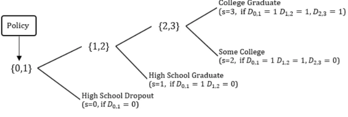
My sequential schooling model includes three transitions (see figure 4.1). At each transition
the individuals choice set includes two alternatives, either transit to the next level of education or
dropout from schooling system.3 I defineJ as the set of possible schooling states, wherejdenotes a possible state available to the individual. In my framework there are four possible states: j = 0
denotes the state of high school (HS) incomplete,j = 1is the state of being a HS graduate,j = 2
is attending college, and j = 3 denotes college graduate. Let Dj,j0 = 1 if a person at state j
chooses to transit to statej0 at the decision node{j, j0}
, wherej, j0, andDj,j0 ∈ D, the set of all
possible schooling decisions taken by an individual. For instance, if an individual at the decision
1This framework was original developed by Cameron and Heckman (2001). An extension is presented by
Heck-man and Navarro (2007). Other applications of this framework can be found in HeckHeck-man, Humphries, Urzua, and Veramendi (2011), Reyes, Rodrguez, and Urza (2013). Similar ideas has been applied in other context such as Cooley, Navarro, and Takahashi (2014).
2My set up satisfies the key condition stated in Cunha et al. (2007) Once an individual in the PACES program
leaves school, he never returns.
3In my data I only observe individuals who continue in the education system or dropout from it. I do not observe
node{0,1}chooses to transit to state j = 1, thenD0,1 = 1. If this individual chooses to stay in
the statej = 0(and not transit to statej = 1), thenD0,1 = 0. If an individual completes the three
possible transitions, thenD0,1 = 1,D1,2 = 1,D2,3 = 1. I also definesas the realized final level of
Figure 4.1: Sequential Schooling Model
schooling, wheres, and S = {0,1,2,3}. For instance, in the last examples = 3 (see figure 4.1), and the individual in the former case, who chooses to stay in the state j = 0(D0,1 = 0), s = 0.
There are four possible final schooling levels: HS dropout (s = 0), HS graduate (s = 1), college dropout (s = 2), and college graduate (s= 3). The optimal decision at node{j, j0}is represented by a threshold-crossing model of the formDj,j0 = 1[Vj,j00], whereVj,j0 is the value perceived by
an individual with current state j of attaining schooling level j0, and 1[.] is the logical indicator function taking the value1 if its argument is true and the value0 otherwise. The value function
Vj,j0 is assumed to be a linear (separable) index ofZ and4
Vj,j0 =Zj,j0βj,j0 +j,j0 if Dj−1,j0−1 = 1 (4.1)
Where {j, j0} = ({0,1},{1,2},{2,3})
, and Zj,j0 is a vector of variables observed by both the
agent and the econometrician that determine the schooling transition decision of an agent at the
4Vytlacil (2006) and Vytlacil (2002) demonstrate that assuming a linear or additively separable latent index
decision node{j, j0}, β
j,j0 is a vector of parameters, andj,j0 is a vector of endowments observed
only by the individual but unobserved by the econometrician. Zj,j0 may include policy variables
that affect the transition from j to j0, for instance a scholarship for high school education (see Figure 4.1), or a subsidy to college tuition. Notice thatV0,1is a reduced form of the value function
given in section 3that comprise all schooling years during the secondary education.5 Each final
level of schooling s is associated with a set of k potential labor market outcomes6 (e.g. wages, have a formal job, number of days worked, poverty status, etc.) given by
Yk,s =Xk,sγk,s+εk,s (4.2)
where Xk,s is a vector of observed variables of the individuals relevant for outcome Yk,s, γk,s is
a vector of parameters, and εk,s is a vector of endowments observed only by the agent. The k
observed outcomesYkcan be written in a switching regression form. DefineHs = 1if s is the final
level of schooling reached by the individual andHs = 0otherwise. Then the observed outcome is
Yk=
3 X
s=0
HsYk,s (4.3)
4.1 Factor structure
In general, there are common unobserved endowments associated with both εk,s andj,j0.7 If
the decision to transit to the next decision node of an agent at a particular decision node j, j0
is correlated with the unobservable gains from the final schooling level, I have a situation with
essential heterogeneity in terms of Heckman et al. (2006).8 In this context essential heterogeneity
5For instance,V
0,1>0means that the choice-specific value functionvt(1)is greater thanvt(0)fort = 1,· · · ,6
which represent the years in the secondary education. If, V0,1 < 0, then vt(1) < vt(0) for some t = 1,· · ·,6.
Similarly forV1,2andV2,3.
6Outcomes may be either continuous or discrete.
7ε
k,sandj,j0 are statistical independent, then the best estimation method is to use linear regressions methods to estimate the parametersγk,sand probit models to estimate the parametersβj,j0. See Maddala (2010) for versions of switching regression models with exogenous and endogenous switching.
8See also Ravallion (2015) for a discussion.
means that individuals make rational choices about whether to transit to the next level of education
based on endowments they know but are unobservable to the analyst, and it is expected that those
agents with higher unobserved endowments are more likely to select into a higher level of education
and experience higher gains from that choice. As a consequence, in general, I cannot identify the
joint distribution of outcomes across level of education, and I am not able to identify the treatment
on the treated parameters or policy relevant parameters discussed in the following sections (see
Carneiro, Hansen, and Heckman (2003), Heckman and Navarro (2007)).
To account for essential heterogeneity I must recover the joint distribution εk,s and j,j0 for
all s = 0,1,2,3. To simplify this task, I impose a factor structure for εk,s and j,j0 that allows
me to recover the joint distribution of(Y0, Y1, Y2, Y3)(see Aakvik, Heckman, and Vytlacil (1999),
Aakvik, Heckman, and Vytlacil (2005) and Carneiro et al. (2003)).
Assumption1: j, j0 = αj,j0θ+vj,j0 andεk,s = αk,sθ+uk,s, whereαk,s andαj,j0 are factor
loadings, θ is a factor that is independent of allvj,j0, uk,s, and observable variables. Also,vj,j0 is
statistical independentvi,i0 for all{j, j0} 6={i, i0},uk,sis statistical independent oful,sfor allk, and
vj,j0 is statistical independent ofuk,s for all{j, j0}andk. I also assume vj,j0, uk,s are independent
distributed random variables with mean zero and finite variance.9
The factor structure also helps me control for dynamic selection, i.e. different types of students
might select into specific nodes over the three decisions based on unobservable characteristics. For
instance, suppose that θ is known and θ = ¯θ. The value of graduating from high school for a student of typeθ¯, at the decision node{0,1}(i.e. V0,1 =Z0,1β0,1+α0,1θ¯+v0,1), may be correlated
with the value of enrollment in college conditional onD0,1 = 1, at the decision node{1,2}(i.e.
V1,2 = Z1,2β1,2 +α1,2θ¯+v1,2). Nonetheless, conditional on , the optimal decision at the node
{1,2}, given byD2,1, is independent of the optimal choice at the node{2,3}, given byD0,1.
4.2 Identification
I define identification in a standard way. In general, the identification of the parametersβj,j0,
γk,s and the distributions Fεk,s,Fj,j0 is possible if there is sufficient variation in the components
(Zj,j0, βj,j0) for each value of the index functions, i.e. there is measurable separability among
the index value functions. In propositions1 and2 in the appendix (see appendix C), I show the
sufficient conditions for the identification of a model specified by Equations(1)and(2)and given
the characteristics of my data, in particular, I exploit the randomization of the scholarship that
affects the first transition.10
These results do not allow me to identify the joint distribution ofY0,Y1,Y2,Y3 because I only
observe one of these outcomes for any individual, which implies that I cannot identify treatment on
the treated parameters. I use the factor structure in assumption1to identify the joint distribution
ofY0,Y1,Y2,Y3 and the policy relevant parameters of interest.
My identification approach exploits the factor structure to control for the possibility of dynamic
selection and essential heterogeneity. I first show how the factor structure allows me to obtain
the conditional independence assumption of quasi-experimental methods. Then, I show how to
identify the joint distribution of εk,s and j,j0 for all s = 0,1,2,3.11 I keep all conditioning on
covariates implicit to simplify notation.
Propositions 1and 2 in the appendix C provide sufficient conditions for the identification of
βj,j0, γk,s and the distributions F
j,j0,Fεk,s for all s, but they are not sufficient to recover the joint distribution ofY0,Y1,Y2,Y3. Assumption1reduces the problem of recovering the joint distribution
εk,s and j,j0 to the problem of recovering the loading parameters αk,s andαj,j0, and the marginal
distribution ofθ,vj,j0, anduk,s.
Now I illustrate the problem using the structure of my schooling model with one outcome
which includes three value index functions and four potential outcomes:
10Sufficient conditions for a other classes of models can be found in Heckman and Navarro (2007), Cunha et al.
(2007), Abbring and Van den Berg (2003),Carneiro et al. (2003).
11See Cunha, Heckman, and Schennach (2010) and Heckman and Navarro (2007) for more general cases.
V0,1 =Z0,1β0,1+α0,1θ+v0,1
V1,2 =Z1,2β1,2+α1,2θ+v1,2
V2,3 =Z2,3β2,3+α2,3θ+v2,3
Y0 =X0γ0+α0θ+u0
Y1 =X1γ1+α1θ+u1
Y2 =X2γ2+α2θ+u2
Y3 =X3γ3+α3θ+u3
(4.4)
I set the scale ofθ by normalizing the factor loadingα0,1 = 1.12 The unobservable gains of a
final schooling levels0with respect toswheres0 > sare given byεs0−εs = (αs0−αs)θ+(us0−us).
Notice thatαs0−αs6= 0implies the presence of essential heterogeneity in my framework because
the unobserved gains are correlated with the errors of the index functions, and then with the optimal
schooling choices (i.e. D0,1,D1,2,D2,3) sinceθ affects both.
I also suppose that the first schooling choiceD0,1 is not correlated with any previous schooling
choice, i.e. it is free of dynamic selection,13 which in turn implies that the parameters ofV
0,1 do
not depend on previous schooling choices. For all other choices the selection process is dynamic
in the sense that transition choice at the node j, j0 depends on the transition choice at the node
j−1, j0−1. For instance, individual choice at node{1,2}is only possible if at the node {0,1}
the optimal choice by the individual wasD0,1 = 1. Since the unobserved endowmentsθinfluence
decisions in consecutive transitions, and given thatα1,2 6= 0,α2,3 6= 0, dynamic selection does not
allow me to identify the model.
12In general, the scale ofθis unknown, sinceθis an unobservable. So any other normalization will be as good as α0,1= 1.
13This assumption is natural in our specific problem since the students who participated in the PACES program
were selected by a lottery mechanism in the first year of high school, so everyone in the sample finished elementary school (see Angrist et al. (2002), Angrist et al. (2006)). Also, the dropout rate for elementary education in Bogota by