USING PATIENT PREFERENCES TO ESTIMATE OPTIMAL TREATMENT STRATEGIES FOR COMPETING OUTCOMES
Emily Lynn Butler
A dissertation submitted to the faculty of the University of North Carolina at Chapel Hill in partial fulfillment of the requirements for the degree of Doctor of Philosophy in
the Department of Biostatistics in the Gillings School of Global Public Health.
Chapel Hill 2016
ABSTRACT
Emily Lynn Butler: Using Patient Preferences to Estimate Optimal Treatment Strategies for Competing Outcomes
(Under the direction of Michael R. Kosorok)
ACKNOWLEDGMENTS
My advisor, Dr. Michael Kosorok, deserves immense acknowledgment and my eternal gratitude for guiding and supporting me not only through the dissertation pro-cess, but throughout my entire time at the University of North Carolina. He has not only been a teacher and a mentor, but an invaluable source of encouragement through frustrating times and an unwavering sense of stability within the department. His patience throughout this process is unmatched and is only surpassed by his immense kindness, both on and off campus. His support of my decision to work remotely im-pacted my education, progress and success tremendously and my only hope is to make him proud by going out into the world and making substantive contributions to the medical and statistical community.
My profuse appreciation is given to Dr. Eric Laber for his guidance, innovation, foresight, and feedback throughout this process. To say this work would not exist without his diligence and contribution is an understatement. I would also like to thank my committee, Dr. Davis, Dr. Edwards, Dr. Zeng and Dr. Cole, for their time, thoughtful input and advice.
have been my cheerleaders since before I can remember and always believed in me when I didn’t believe in myself. This accomplishment is not only mine, but is theirs, and I could not have had a better team in my corner. Finally, to Briana and Jenny, the emotional support and levity you have provided, especially in moments of despair, is incalculable; your friendship is one of the greatest gifts I have the honor of leaving UNC with.
TABLE OF CONTENTS
LIST OF TABLES . . . x
LIST OF FIGURES . . . xi
CHAPTER 1: INTRODUCTION ⋅ ⋅ ⋅ ⋅ ⋅ ⋅ ⋅ ⋅ ⋅ ⋅ ⋅ ⋅ ⋅ ⋅ ⋅ ⋅ ⋅ ⋅ ⋅ ⋅ ⋅ ⋅ ⋅ ⋅ 1 CHAPTER 2: LITERATURE REVIEW ⋅ ⋅ ⋅ ⋅ ⋅ ⋅ ⋅ ⋅ ⋅ ⋅ ⋅ ⋅ ⋅ ⋅ ⋅ ⋅ ⋅ ⋅ ⋅ ⋅ 5 2.1 Introduction . . . 5
2.2 Item Response Theory . . . 7
2.3 Study Design . . . 11
2.4 Variable Selection . . . 20
2.5 Analysis Techniques: Single Stage . . . 23
2.6 Analysis Techniques: Multiple Stages . . . 31
2.7 Observational Data . . . 41
2.8 Competing Outcomes . . . 47
2.9 Conclusion . . . 51
CHAPTER 3: INCORPORATING PATIENT PREFERENCES INTO ESTI-MATION OF OPTIMAL INDIVIDUALIZED TREATMENT RULES ⋅ ⋅ ⋅ ⋅ ⋅ ⋅ 52 3.1 Introduction . . . 52
3.2 Optimal ITRs with Heterogeneous Patient Preferences . . . 55
3.2.1 Setup and Notation . . . 55
3.2.2 Estimating an Optimal ITR . . . 57
3.3 Simulation Study . . . 60
3.3.1 Data Generating Model . . . 61
3.3.2 Simulation Results . . . 61
3.5 Discussion . . . 66
CHAPTER 4: ESTIMATING DYNAMIC TREATMENT STRATEGIES BY INTEGRATING PATIENT PREFERENCES ⋅ ⋅ ⋅ ⋅ ⋅ ⋅ ⋅ ⋅ ⋅ ⋅ ⋅ ⋅ ⋅ ⋅ ⋅ ⋅ ⋅ ⋅ 67 4.1 Introduction . . . 67
4.2 Estimating the Optimal DTR . . . 69
4.2.1 Framework . . . 69
4.2.2 Methodology . . . 72
4.3 Simulation Study . . . 75
4.3.1 Data Generating Model . . . 75
4.3.2 Simulation Results . . . 77
4.4 Discussion . . . 79
CHAPTER 5: NONPARAMETRIC INCORPORATION OF PATIENT PREF-ERENCES FOR INDIVIDUALIZED TREATMENT RULE ESTIMATION ⋅ ⋅ ⋅ 81 5.1 Introduction . . . 81
5.2 Optimal Nonparametric ITRs with Patient Preferences . . . 83
5.2.1 Framework and Notation . . . 83
5.2.2 Estimation . . . 85
5.3 Simulation Study . . . 90
5.3.1 Setup and Assumptions . . . 91
5.3.2 Simulation Results . . . 91
5.4 Discussion . . . 94
CHAPTER 6: DISCUSSION ⋅ ⋅ ⋅ ⋅ ⋅ ⋅ ⋅ ⋅ ⋅ ⋅ ⋅ ⋅ ⋅ ⋅ ⋅ ⋅ ⋅ ⋅ ⋅ ⋅ ⋅ ⋅ ⋅ ⋅ ⋅ ⋅ 96 APPENDIX A: DETAILS FOR CHAPTER 3 ⋅ ⋅ ⋅ ⋅ ⋅ ⋅ ⋅ ⋅ ⋅ ⋅ ⋅ ⋅ ⋅ ⋅ ⋅ ⋅ ⋅ ⋅ 99 A.1 Consistency Proof Details . . . 99
A.2 Comparison of ̂µM HE,n(x,w)and ̂µM oME,n (x,w) Details . . . 110
A.3 Case Study Details . . . 112
LIST OF TABLES
3.1 Treatment recommendations ⋅ ⋅ ⋅ ⋅ ⋅ ⋅ ⋅ ⋅ ⋅ ⋅ ⋅ ⋅ ⋅ ⋅ ⋅ ⋅ ⋅ ⋅ ⋅ ⋅ ⋅ ⋅ ⋅ ⋅ 65
LIST OF FIGURES
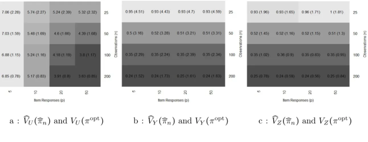
3.1 Averaged squared difference: V̂
U(̂πn) , V̂Y(̂πn) and V̂Z(̂πn) ⋅ ⋅ ⋅ ⋅ ⋅ ⋅ ⋅ ⋅ 62
3.2 Average percent disagreement: ̂πn, πopt and πoracle ⋅ ⋅ ⋅ ⋅ ⋅ ⋅ ⋅ ⋅ ⋅ ⋅ ⋅ ⋅ ⋅ 62
4.1 Average percent disagreement: ̂πD2, π2T and ̂π2S ⋅ ⋅ ⋅ ⋅ ⋅ ⋅ ⋅ ⋅ ⋅ ⋅ ⋅ ⋅ ⋅ ⋅ ⋅ 78
4.2 Average percent disagreement: ̂πD1, π1T and ̂π1S ⋅ ⋅ ⋅ ⋅ ⋅ ⋅ ⋅ ⋅ ⋅ ⋅ ⋅ ⋅ ⋅ ⋅ ⋅ 79
5.1 Mean squared error: G=Φ(E) and ̂µn(x,w) ⋅ ⋅ ⋅ ⋅ ⋅ ⋅ ⋅ ⋅ ⋅ ⋅ ⋅ ⋅ ⋅ ⋅ ⋅ 92
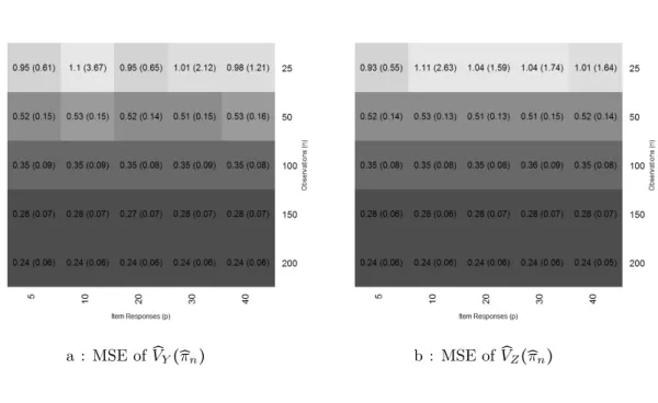
5.2 Estimated and true piecewise linear splines forµn(x,w) =h(G). ⋅ ⋅ ⋅ ⋅ ⋅ 92 5.3 Mean squared error: V̂
Y(̂πn) and V̂Z(̂πn) ⋅ ⋅ ⋅ ⋅ ⋅ ⋅ ⋅ ⋅ ⋅ ⋅ ⋅ ⋅ ⋅ ⋅ ⋅ ⋅ ⋅ 93
5.4 Mean squared error: V̂
U(̂πn)and πopt ⋅ ⋅ ⋅ ⋅ ⋅ ⋅ ⋅ ⋅ ⋅ ⋅ ⋅ ⋅ ⋅ ⋅ ⋅ ⋅ ⋅ ⋅ ⋅ 94
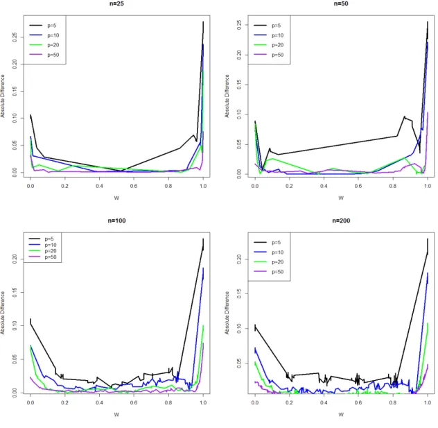
6.1 Absolute difference: ̂µM HE,n(x,w) and ̂µM oME,n (x,w) ⋅ ⋅ ⋅ ⋅ ⋅ ⋅ ⋅ ⋅ ⋅ ⋅ ⋅ ⋅ ⋅ 111
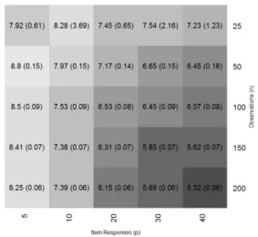
6.2 Averaged absolute and mean difference: ̂µM HE,n(x,w) and µ̂M oME,n (x,w) ⋅ ⋅ ⋅ 112
6.3 Mean squared error: G=Φ(E) and ̂µn(x,w) ⋅ ⋅ ⋅ ⋅ ⋅ ⋅ ⋅ ⋅ ⋅ ⋅ ⋅ ⋅ ⋅ ⋅ ⋅ 115
6.4 Mean squared error: V̂
Y(̂πn) and V̂Z(̂πn) ⋅ ⋅ ⋅ ⋅ ⋅ ⋅ ⋅ ⋅ ⋅ ⋅ ⋅ ⋅ ⋅ ⋅ ⋅ ⋅ ⋅ 116
6.5 Mean squared error: V̂
CHAPTER 1: INTRODUCTION
Advancements in many areas have contributed to the vast incorporation of pre-cision medicine in current patient treatment plans. This includes, but is not limited to, genetically determining which biomarkers are associated with particular diseases (Jain 2002), increased efficiency of drug delivery systems (Allen and Cullis 2004), and more complex data collection procedures which provide richer data to make inference on (Cai et al. 2011). The goal of precision medicine is to incorporate a parsimonious amount personalized information to efficiently determine which treatments are best for which types of patients (Norvig et al. 2010, Hamburg and Collins 2010). This re-sults in strategies that treat particular diseases by targeting a certain genetic marker, strategically controlling the amount and frequency of dosages and determining which patients should be receiving which treatments based on their demographic and clinical information.
and side effect burden, or even quality of life and cost. There are currently three primary approaches to estimation of optimal individualized decision rules for competing outcomes: (i) set-valued treatment regimes (Laber et al. 2014b, Lizotte and Laber 2016); (ii) inverse-preference elicitation (Lizotte et al. 2012a) ; and (iii) constrained estimation (Linn et al. 2016). Each of these either assumes a fixed composite outcome or does not address patient preferences directly through elicitation.
While the ideal situation is to directly elicit patient preferences, the type of elic-itation where the patient chooses parameters to define a composite outcome is not feasible unless patients have undergone specialized training (Brennan 1998, Braziunas 2006, Lizotte et al. 2012a). Thus, the preferences must be indirectly estimated from information that can be directly obtained. A common approach for preference elicita-tion is to administer an itemized queselicita-tionnaire that characterizes how the patient feels about each outcome in relation to the other. We assume the questionnaire is comprised of a series of binary responses to each question and use item response theory (Embret-son and Reise 2013) to estimate the conditional distribution over these preferences. We use this conditional distribution to derive preference-sensitive optimal individualized treatment strategies for each patient.
1980). This preference information is standardized and incorporated into a linear util-ity function. The optimal treatment rule is that which optimizes the expected utilutil-ity function for a given set of patient covariates. The second method extends this to the multiple stage scenario where the preference information is updated at each treatment stage based on how a patient’s preferences have changed and their overall contentment with their health status. Using a reinforcement learning technique called Q-learning (Watkins and Dayan 1992), the optimal treatment rule is determined as that which provides the maximum expected utility given the patient’s history, assuming that the best treatment is assigned at all subsequent stages. The final method provides a more flexible estimator by solving this problem nonparametrically. The preference informa-tion is condiinforma-tioned on the itemized responses through constrained monotonic splines (Villalobos and Wahba 1987). To estimate the patient’s ideal trade off between the two outcomes, we define a nonparametric utility function using monotonic splines once again to calibrate the patient’s satisfaction with the outcomes after receiving the treat-ment. This more accurately captures the patient’s feelings on how to weigh the two outcomes.
debilitating mental disorder that may make patients lose touch with reality and can af-fects mental cognition, emotional stability and social behaviors (Andreasen and Flaum 1991). Since it cannot be cured at this time, treatments are designed solely to alle-viate symptoms. One of the main treatments for schizophrenia is the administration of antipsychotic medications. Some of these antipsychotics elicit negative side effects in the patient, making it difficult for them to adhere to the treatment regimes, while others are less efficacious but also have less side effects (Lieberman et al. 2005). It is important to develop treatment plans that can find the appropriate balance between relieving schizophrenic symptoms and reducing the side effect burden. We can use this example to provide a realistic scenario when generating data for our simulation study. While this is one example of the application for this work, similar comparisons can be made with diseases such as rheumatoid arthritis and diabetes.
CHAPTER 2: LITERATURE REVIEW
2.1 Introduction
tailoring variables to the intervention options at decision points) (Collins et al. 2014). In the statistical framework, DTRs are developed to create mathematically de-pendent treatment plans that mimic how clinicians treat patients in practical settings. This quantitative way of estimating treatment plans is a new and novel way to think of treating patients. Preliminary interest in this way of thinking began in the mid-1980s when researchers were evaluating two stage dynamic treatment strategies for cancer pa-tients. In the 1990s the idea of a two stage customized treatment plan expanded when psychiatrists were interested in expanding to k-stage treatment plans. By the early 2000s, clinical trials and treatment strategies were implemented by doctors studying DTRs in substance abuse and mental health research (Lavori and Dawson 2014). Once the physician or researcher has conjured a list of potential DTRs, they need to be evaluated in a special clinical trial called a Sequential Multiple Assignment Random-ization Trials (SMART) (Murphy 2005a). The development of SMARTs began when traditional clinical trial designers were looking to identify an intermediate outcome be-tween randomization and the primary outcome and make an appropriate reaction to this outcome. The goal was to be able to assess the status of the patient throughout the trial and adjust the treatment as necessary.
The material presented in this literature review is meant to be a survey of current statistical methods used to estimate dynamic treatment regimes in the context of using data collected in a SMART trial. Chakraborty and Moodie (2013) have published a book titled “Statistical Methods for Dynamic Treatment Regimes” which covers this and similar topics in some depth. In this book, the authors discuss select topics such as SMART designs, observational studies, reinforcement learning and various methods of estimating DTRs. Please refer to this book for an indepth description of a number of useful methods for DTRs.
This review covers a brief introduction to item response theory, how to design a SMART and what statistical methodologies exist to make inference from this data, with particular emphasis on recent developments in the area. Section 2.2 introduces item response theory and the Rasch model. Section 2.3 will highlight how a SMART design fits into the overall development of a treatment strategy, the importance of pilot studies, practical considerations such as sample size, calculations, and handling missing data, as well as the future of data collection. Section 2.4 describes select methods for choosing tailoring variables. Section 2.5 introduces methodological results for the single stage paradigm and section 2.6 provides methodological results for the multiple stage paradigm. Section 2.7 describes methods designed to develop DTRs when the only data available is observational because a randomized design is not practical, is impossible, or is unavailable. Section 2.8 describes the work done developing DTRs for competing outcomes.
2.2 Item Response Theory
will be employed to estimate a subject’s implicit utility function regarding the two competing outcomes so that it can be included in estimation. This is done by estimating parameters from the Rasch model that is conditional on a unidimenional latent trait.
Item response theory (IRT) concerns the accuracy and development of test scoring when these tests or questionnaires are designed to measure abilities, traits, or behaviors (An and Yung 2014). The test or questionnaire consists of a set of items (questions) with binary or ordinal responses. These models not only provide accuracy of test scoring, but can also improve efficiency of data collection by only including the significant items. Historically, IRT has been primarily used for psychological assessments and educational testing, but these models have recently been extended to health research. This is partially because of the aforementioned ability to tease out only the discriminative items for inclusion. Outside of the education and psychological areas, IRT is referred to as Latent Trait Modeling (LTM).
but computationally they are essentially the same.
IRT is advantageous over classical test theory (CTT), one of the original methods of test response analysis, because IRT takes both information from the person and the items into account (Yu 2013). CTT cannot differentiate between the subjects profi-ciency and the difficulty of the item; meaning for populations of different proficiencies, the questionnaires could seem easy or difficult (An and Yung 2014). On the other hand, IRT assesses both the difficulty of the question and the subject’s proficiency through-out the entire questionnaire. Once the items are calibrated for the population, scores for subjects can be compared even if they did not answer the same set of questions. This calibration requires an iterative process because the proficiency and difficulty de-termined by the data are used to fit the model which in turn predicts the data. The ability to compare subjects who respond to different sets of items also reduces the size of the questionnaire. This increases efficiency and in turn reliability because the precision differs based on latent structure and can be generalized to the entire population. IRT modeling is considered a superior analysis method and is employed in many standard-ized exams, such as the Scholastic Assessment Test (SAT) and the Graduate Record Examination (GRE) (An and Yung 2014).
The one parameter Rasch model is designed for dichotomized response data, i.e
{1,0} where 1 corresponds to “yes" and 0 corresponds to “no". The probability of
responding “yes" is:
P(xij =1∣θi, βj) = e
θi−βj
1+eθi−βj
whereP(xij=1∣θi, βj) is the probability of personi responding “yes" (1) to question j
(Li and Baron 2012). The latent trait, θi, is thought of as person i′s proficiency and
βj represents the difficulty of item j. The probability of answering yes to each item is dependent on the person’s proficiency and item’s difficulty such that if the person’s proficiency matches the item’s difficulty, that person has a 50% chance of answering yes.
The Rasch model can be extended to a two parameter model by introducing a dis-crimination parameter, which measures the slope, to allow more flexibility in modeling (An and Yung 2014). In this model, the probability of responding “yes" is:
P(xij =1∣θi, βj) = e
αjθi−βj
1+eαjθi−βj
where the discrimination parameter, αj, measures if the item has the ability to dif-ferentiate subjects. A high discrimination parameter (αj) implies that the probability of answering "yes" increases more rapidly as the proficiency parameter (βj) increases. This parameter tells how effectively the item discriminates between highly and lowly proficient students (Yu 2013)
not limited to, three and four parameter models, Bayesian IRT models, models used to analyze ordinal responses (graded response models), and models used to analyze items that can be explained by more than one latent trait (multidimensional models).
Letting πij =P(xij =1∣θi, βj), the Rasch model can easily be transformed into a logistic regression model (or a probit model) such that:
logit(πij) =αjθi−βj
where θi is the latent variable and αj, βj are parameters that can be estimated from the data.
2.3 Study Design
evaluated in a traditional randomized controlled trial (RCT) where they investigate efficiency and practicality. At times the first two phases need to be repeated before the final stage can be implemented. The MOST assumes that experimentation makes the most efficient use of available resources with the goal of producing the largest improve-ment and treats optimization as a process rather than an endpoint.
Traditionally, the screening/preparation and refining/optimization phases used a factorial or fully crossed analysis of variance (ANOVA) design. Because SMART designs are considered a special case of the factorial design where not all factors need to be crossed, they have been found to be advantageous to replace the ANOVA model in the second phase. A SMART creates the adaptive intervention by allowing for dynamic treatments (as opposed to fixed ones) and provides a basis to identify the best tailoring variables and decision rules. Recall that tailoring variables are essentially patients’ prognostic information used to make treatment decisions and the decision rule is a way of choosing which treatment to assign. They investigate the best sequencing of intervention components, what tailoring variables should be used, when and how frequently should these tailoring variables be assessed, and should one treatment be assigned or should patients have the ability to choose from a list of options. The treatments are assessed as an entire treatment sequence and not isolated by phase of treatment. They involve multiple randomizations over time, where each randomization point corresponds to a decision point and questions are investigated regarding two or more treatment options at each decision point. Additionally, responders and non-responders are controlled for by design because different treatment decisions need to be considered for each (Collins et al. 2007; 2014).
and 100 patients to treatment B at stage 1. At the end of stage 1 the patients’ re-sponse to the treatment is assessed using the rere-sponse variable or tailoring variables, and the patients are classified as either responsive or nonresponsive. What defines re-sponsive or nonrere-sponsive should be determined a priori. Each of the patients is then re-randomized according to their response classification. For instance, patients who responded to treatment A are assigned to stay on treatment A at stage 2, while the patients who did not respond to treatment A are randomized to treatment C or D. A similar situation could arise for treatment B where responders stay on treatment B and nonresponders are randomized to treatments E or F. In this scenario, there are 6 DTRs: A-A A-C A-D B,B B,E B,F. Alternatively, responsive patients could also be re-randomized. There could be more than 2 randomization options at each stage, or the nonresponsive patients could switch from A to B or vice versa. The randomization also does not need to be balanced, and the stages could be extended beyond only 2. In this example data would be collected at 3 time points: baseline, time 1 (after the first stage of the study but before the patient is re-randomized to the second treatment), and time 2 (after the second stage or at the end of the study). Generally speaking, randomization does not need to depend on responder status, although this is the case in this example.
to compare the embedded treatment regimes that pool information across multiple experimental conditions by, again, recycling patients through the trial (Collins et al. 2014). While the main goal of a SMART is to mine data used to develop DTRs, they have other uses, such as discovering which treatments work best sequentially to obtain an improved outcome, investigating the interplay between trajectories of the patients disease progression and treatment sequences, comparing different treatment sequences, and investigating the benefit of both prognostic information and observable data in determining individualized treatments (Almirall et al. 2012).
additional potential tailoring variables should be collected, such as either baseline pa-tient characteristics or time varying measures. These are determined as important in predicting outcomes to later stage treatments; (3) deciding how to control for missing tailoring variables. This should be guided by how it would be handled in clinical prac-tice; (4) deciding between up-front randomization (randomization at the beginning of the trial) or real-time randomization (randomized sequentially at each decision point which allows for clinical information to be used in randomization); (5) highlighting the difference between research assessments for data analysis to develop adaptive treat-ment strategies and assesstreat-ments of the adaptive treattreat-ment strategies used to inform the sequential treatment assessment; (6) identifying concerns clinicians have regarding sequences of treatments offered and assessment of what determines response versus nonresponse; (7) assessing for patient acceptability; (8) testing the language of consent forms; (9) illuminating unanticipated tailoring variables that would be useful in the subsequent SMART.
feasible for patients with toxicity or disease progression. They altered one of the DTRs to include those patients who had to leave the study because of toxicity where the second treatment was the recovery treatment they were given after leaving the trial. The viable DTRs were now defined by efficacy, toxicity and disease progression. The authors also redefined this endpoint because it needed to quantify the health experience of the patient over a pre-specified fixed period, not just their final tumor size or toxicity. By now it should be clear that designing, implementing and analyzing SMARTs is a relatively new area, which means there is still a lot of work to be done. While there is a lot of methodological work needed or expanded upon (see subsequent sections), there are still a lot of gaps in knowledge for designing these trials. One clear gap in the literature is work on a universal (or adaptable) sample size formula. There are sample size calculation publications for SMART designs, but there is no universally accepted calculation for general use.
the log rank statistic (nL) are
nK≤
(Z1−α/2+Z1−β)2σB2 {F¯1(τ) −F¯2(τ)}
2
and
nL≤ (
1
pq+
1 (1−p)q
)
(Z1−α/2+Z1−β)2
ξ2´t
0F¯c(t)dF1(t)
respectively, where Z is the z-score for a standard normal distribution, α is the type I error, β is the type II error, F¯ is the survival function,τ is the time at the end of the study, p=p(A1 =1) and q=p(A2 =1∣R =1) are the randomization probabilities, R is
the indicator of randomization, ξ is the log hazard ratio. Note that
σ2B= ¯
F2 1(τ)
pq
ˆ τ
0
dΛ1(t) ¯
F1(t)F¯c(t) +
¯
F2 2(τ) (1−p)q
ˆ τ
0
dΛ2(t) ¯
F2(t)F¯c(t)
where Λ is the cumulative hazard function. This sample size calculation has been
proven to provide the desired power if the hazards of the alternative are proportional. This sample size calculation is most notable because the nature of chronic diseases (the focus of SMARTs and DTRs) allows the outcome, or surrogate outcome, to be thought of in terms of failure, even if death is not the primary endpoint. This means that this sample size formula will be applicable in many settings, especially until further research is done.
presents unique challenges when analyzing data in the presence of missing data. Impu-tation strategies for handling missing data collected from SMARTs is an understudied area at this time. Shortreed et al. (2014) presented the following five missing data issues: (1) transition between treatment stages does not always occur at pre-specified times but instead can be determined by a patient outcome; (2) some outcome variables are irregularly spaced while some variables are collected at regularly scheduled study visits; (3) observing some variables is dependent on a patient’s history, which results in structural missingness for the data-dependent portion of the collected information. (4) individuals are simply lost to follow up leaving the treatment stage; (5) some indi-viduals are lost to follow up entering the treatment stage. Their proposed solution is a flexible imputation strategy to facilitate valid inference using data from SMARTs which is a time ordered, nested, conditional imputation strategy, which exploits the nearly monotone pattern of missing data found in this type of longitudinal study. It ensures that a complete multivariate prediction distribution exists while obtaining desirable traits for inference across longitudinal outcomes. Assuming missingness at random, this method works best when the data is imputed with a pseudo-Gibbs sampler, which applies repeated iterations through the model. Multiple imputation is one of many strategies used when working with missing data, and the type of strategy often de-pends on the structure of the data and the nature of the missingness. This method was not compared to other imputation strategies such as inverse probability weighting or likelihood methods, and there is no contingency plan when the missingness is not monotone. It is clear the presented work is exciting and promising progress, but more headway is still needed.
(which will be covered in later sections). Even though this concept is in the early stages of development, there are obvious feasibility issues for this kind of treatment implementation, such as cost and monitoring adherence. Innovative methods like this have the ability to change the way patients are treated and can serve as a guide for future treatment and collection methods.
A SMART is a novel approach to efficiently collect data which accurately esti-mates DTRs for individualized patients. The basic design structure has been created, trials are ongoing in the clinical setting, and new advances are being developed day by day, but more work needs to be done. The flexibility of the design makes developing broad techniques difficult, but the need and the talent is there to continue to make advancements in what has become an extremely timely, interesting and applicable area of study.
2.4 Variable Selection
Variable selection is an important component of estimating optimal DTRs because tailoring variables are used to adapt the treatment plan to the individual. The goal is to avoid a priori hand picking tailoring variables, but instead use the data to select a subset of the tailoring variables that estimates a decision rule as close to the optimal rule estimated when using all variables. Including all possible variables as tailoring variables is inefficient and will often lead to over fitting. Once the tailoring variables are selected, they can be used when optimizing DTRs. A brief overview of recent and relevant variable selection techniques is included in this section.
the treatment based on the value of that variable. It combines the interaction of the covariate with the treatment and the proportion of the population exhibiting variability in that covariate. Higher values indicate stronger relationships between the variable and the treatment, and shows that a large proportion of patients would experience change in the optimal action if the variable was taken into consideration. This scoring is used to rank potential variables but each variable is evaluated separately meaning correlation between variables is not taken into consideration. The S-score could also be used sequentiality such that the variable with the highest score is first selected, then the variable with the second highest score given the first variable is selected and so on. The reducts approach was developed from rough set theory in computer science. The positive region is a set of all observations that can be uniquely classified into one equivalence class based on the non-decision variables. The reduct is the minimal set of tailoring variables that classifies individuals into unique decision equivalence classes as well as the complete set of variables does. Reducts help eliminate redundant variables while preserving information regarding the similarity of individuals in the sample. In the scenario with multiple reducts, one can select the variables most frequently seen in the reducts, or can select amongst reducts by choosing the set of covariates with the highest S-score. This last hybrid method is believed to combine the strengths of these two methods. Unfortunately, it is important to note that reducts are not appropriate for continuous outcomes.
quickly implementable with current software. The authors suggest the loss function
Ln,φ(β, γ) = 1
n n
∑
i=1
[Yi−φ(Xi;γ) −βTX˜i{Ai−α(Xi)}] 2
where n is the number of observations, Yi is the ith patient’s outcome, Xi is the ith patient’s prognostic variables, X˜ = (1, XT)T, A
i ∈ {−1,1} represents the dichotomous treatment choice, α(x) denotes the propensity score, and φ is an arbitrary function
with a constant model for φ ∶ φ(x;γ) = γ and a linear model for φ ∶ φ(x;γ) = γTx˜.
This characterization of the loss function increases simplicity in adopting shrinkage penalties for variable selection. Employing the adaptive lasso penalty (or, alternatively, the SCAD or minimax concavity penalty) the solution is theβ which satisfies
min
β Ln,φ
(β,˜γ) +λn
p+1 ∑
j=1
wj∣βj∣
where λn is a tuning parameter and wj are the weights such that w−1
j = ∣βj˜∣ is used. Aside from estimating the optimal DTR, these β values are used to determine which variables are important in selecting the optimal DTR such that the important variables are those with nonzero coefficients.
2.5 Analysis Techniques: Single Stage
The list of methodology presented here and in the subsequent section is neither complete nor representative of all available options, but a simple summary of recent or relatively recent methods employed along a broad range. The purpose is to introduce popular techniques, highlight advancements, and display a plethora of methodological options applicable in multiple areas of interest.
Important notation must be introduced so that an individualized treatment rule (ITR) for the single stage paradigm can be properly defined. An ITR differs from a DTR in that it is the personalized rule for a single treatment setting while a DTR is the sequence of decision rules for a multiple treatment setting. Assuming the data is collected from a single stage two arm trial, the treatments will be annotated as A ∈ {−1,1}. These are independent of the patient prognostic variables denoted as
X = (X1, . . . , Xp)T, where X is a p-dimensional matrix. In the single stage paradigm
the observed clinical outcome, Y, can be considered a reward function where larger values are desired. The ITR is a map from the prognostic variable space, X, to the treatment space,A, and the optimal ITR is theAwhich maximizes the expected reward. The distribution of (X, A, Y)is denoted byP with the respective expectation denoted
asE. The distribution of(X, A, Y) given the ITR,D(i.e. thatA=D(X)), is denoted
asPD and the corresponding expectation as ED. The expected reward under D is
V(D) =ED(Y) =E[
I{A=D(X)}
Aπ+1−2A
Y]
whereπ=P(A=1). This V(D)is referred to as the value function for a givenD. The
D∗
∈argmaxDV(D) =argmaxDE[I
{A=D(X)}
Aπ+1−2A
Y]
and is considered the D which maximizes the value function V(D). The optimal
treatment regime is defined as the one that maximizes the average expected outcome (Zhao et al. 2012).
One way to estimate ITRs is to restructure the estimation procedure into a clas-sification problem where the optimal classifier corresponds to the optimal treatment decision. The optimal classifier can be found by estimating the Bayes classifier, which is the one that minimizes the expected weighted misclassification error. This frame-work allows for estimation of mean outcomes under existing methods such as regres-sion estimation, inverse probability weighted estimation (IPWE) or augmented inverse probability weighted estimation (AIPWE) (Zhang et al. 2012a). The class of treatment decisions is data driven because it is chosen by minimizing the L1 the expected weighted misclassification error and does not need to be prespecified.
Define the contrast function as
C(X) =µ(1, X) −µ(−1, X)
which can be thought of as the mean difference between treatment options for a given set of prognostic variables. The optimal ITR estimation problem can be transformed into a weighted classification problem such that the optimal treatment ruleD∗ is found
D∗
=argmaxDE[D(X)C(X)] =argmaxDE(∣C(X)∣ [I{C(X) >0} −D(X)]2)
This means that the optimal treatment rule, D∗, is found to be the one that
maxi-mizes E(∣C(X)∣ [I{C(X) >0} −D(X)]2), which is a weighted classification problem.
Each subject belongs to two classes such that class Z = 1 contains those subjects
who would benefit more from treatment A = 1 as opposed to treatment A = −1, e.g.
µ(1, X) >µ(−1, X), and Z =0 the opposite. Each observation is also given a weight,
W = ∣C(X)∣, which is the loss that would incur from misclassification. Hence, the
optimal ITR is simply the expected weighted misclassification error under the classifi-cation rule D(X). Within this classification construct, the problem then decomposes
into two critical steps. First, one must construct a suitable estimator of the contrast function, using regression, and then invert this to find the estimated optimal treatment rules with an interpretable form using classification methods. This can be extended to the multiple stage scenario as well. This classification prospective falls under the machine learning umbrella. Machine learning, most specifically reinforcement learning, has recently been implemented since it sidesteps the problem of completely modeling the underlying generation model as is necessary in some estimation techniques. Rein-forcement learning is a dynamic programming system that decides which actions need to be taken to optimize a given reward.
Qian and Murphy (2011) propose a modification of this which first estimates the conditional mean response using l1 penalized least squares (l1-PLS) with a rich linear
from the optimal treatment rule and the mean response from the estimated treatment rule holds even if the linear model for the conditional mean response is incorrect. If the part of the conditional mean model involving the treatment effect is correct then the upper bounds imply that the estimated treatment rule is consistent. These upper bounds can also inform how to choose the tuning parameters involved in thel1-penalty
to create the best rate of convergence. To obtain the ITR the estimated prediction error is minimized then the conditional mean model is maximized over the treatment A. To control for overfitting, l1 penalized least squares is implemented since the l1
penalty innately does variable selection. The resulting treatment rules are cheaper to implement and easier to interpret.
single stage setting due to the associated reduced bias (Zhao et al. 2012).
Zhang et al. (2012b) approaches estimating dynamic treatment rules by assuming a posited regression model. This defines the class of treatment rules while recognizing that it is possible for the model to be misspecified. The optimal treatment regime is estimated by directly maximizing the estimator for the overall population mean outcome under all possible specified treatment plans using a suitable inverse probability weighted estimator. When using observational data, this estimator has the ability to control for possible confounders by estimating propensity scores and exploiting the predicted outcome, which ensures precision of the estimate. Let D∗ be the optimal
treatment decision, which is the one that corresponds to the largest value ofE[Y∗(D)],
where
Y∗
(D) =Y∗(1)D(X) +Y∗(−1) {1−D(X)}
is the potential outcome. The potential outcome is the outcome that would be observed if a randomly chosen patient were to receive treatment regime D. Consider treatment rules of the formDη(X) =D(X, η) in the class of all possible treatment rules which is
indexed byηand will containD∗ ifµ
(A, X;β)the posited regression model is correctly
specified. Therefore, estimatingη∗=argmax
ηE[Y∗(Dη)] and definingDη∗=D(X, η∗) will provide an estimator forD∗. To estimateE
[Y∗(Dη)], an IPWE or a doubly robust
AIPWE can be employed. This estimator is directly maximized in η to obtain an η∗
and hence Dˆ∗
η(X) = D(X,ηˆ∗). This can easily be extended to the multiple decision situation by estimatingQ(η) =E[Y∗(Dη)]as a function of η.
difference between subjects with observed high and low rewards so that the determina-tion of the actual treatment decisions is associated with the actual treatments received for the different groups. This method is referred to as outcome weighted learning (OWL or O-learning). Developed by Zhao et al. (2012), O-learning is a nonparamet-ric approach which directly optimizes the value function V(D) where each subject is
weighted proportional to their clinical outcome divided by the propensity score, which is the probability of receiving the assigned treatment given the covariates. In the case of a clinical trial, the propensity simplifies to the constant probably of receiving the assigned treatment. Finding theD∗ that maximizes V
(D) =E[I{A=D(X)}
Aπ+1−A2 Y
] is
equiv-alent to finding the D∗ that minimizes V¯(D) =E[I{A≠D(X)}
Aπ+1−A2 Y
] which sets the stage
to view this as a weighted classification error. Minimizing the previous expected value can be approximated by minimizing
n−1 n
∑
i=1
Yi Aiπ+1−2Ai
I[Ai≠sign{f(Xi)}]
to find the optimal f∗ and then setting
D∗
(x) =sign{f∗(x)}
sinceD∗
(x)can always be represented assign{f∗(x)}. This implies the goal is to find
n−1 n
∑
i=1
Yi Aiπ+1−Ai
2
{1−Aif(x)}++λ∣∣f∣∣2
where x+
= max(x,0), and ∣∣f∣∣ is the norm of f. Therefore, this problem is now
a weighted classification problem that can be solved using support vector machine methods.
O-learning has many applications but there are also many ways to extend this line of thinking. Chen et al. (2016) presented a one stage clinical trial design for penalized dose finding using a robust analysis method based on the O-learning framework. The method converts the individualized dose selection problem into a penalized weighted regression with truncated l1 loss. The dose level is assumed to be found on a
contin-uum and a non-trivial extension of O-learning for binary treatments is proposed. The dose finding problem becomes a weighted regression with random outcome where the individual responses are the weights. In the linear case, this framework has the goal of minimizing the loss plus penalty of the form
min
f {
1
n n
∑
i=1
Rilφ{Ai−f(Xi)} 2φnp(Ai∣Xi)
+λn∣∣f∣∣ 2
}
where φ=φn is non-random parameter in real space, λn controls the severity of
the penalty on f, lφ{Ai−f(Xi)} = min(∣A−fφ(X)∣,1), R∗(a) is the potential outcome
and R =
´
I(A=a)R∗(a)p(a∣x)da. The complexity of f(x) is penalized to prevent
S= λn 2 ∣∣w∣∣
2 2+
1
φn n
∑
i=1
Rimin(
∣Ai=D(Xi)∣
φn
,1)
whereλnis now the tuning parameter. This algorithm minimizes the sequence of convex sub-problems with the intent of solving the original non-convex minimization problem. Therefore, the convex sub-problem becomes a weighted penalized median regression problem. Ultimately, the algorithm concludes when ∣∣wt+1−wt∣∣ is smaller
than some prespecified constant, where w= ∑i∈T(αi−α¯i)xi. Expanding to the
nonlin-ear framework, the decision function then becomes a function ofwand some unknown transformation onX. A Gaussian kernel is used to construct a dual problem for nonlin-ear lnonlin-earning that is solved using quadratic programming. To practically implement this procedure, a nonconvex loss function and a DC algorithm for optimization is employed. Another common and extremely relevant application of O-learning is estimating ITRs for censored data. Realistically many chronic diseases measure short term success of a treatment as a failure or success. It is desirable to develop methods of estimating treatment regimes that are applicable to survival analysis because it has clear relevance to personalized medicine. When considering censored data, notation is slightly altered. The value function is redefined as
V(D) =ED(T) =E(T∣X, A=D(X)) =E[I
{A=D(X)}
Aπ+1−2A
T]
where T =min(τ,T˜) where T˜ is the survival time and τ is the end of the study (Zhao
et al. 2015). Even though the outcome is redefined, the optimal treatment rule is still the treatment rule which maximizes the value function. The goal is to estimate D∗
for right censoring, the estimated mean survival time is reassigned as the weighted mis-classification rate. These weights are comprised of both the observed outcome and the inverse probability of censored weights. To offset bias from a misspecified censoring model, a second method, a doubly robust variation of outcome weighted learning, is formulated. In both instances, the treatment rule is consistent for the optimal rule when the model for either the survival times or censoring times is correctly specified. Note: it is not required that both models be correctly specified. A convex relaxation idea from support vector machines is invoked for construction of the necessary estimation algorithm.
The methodological techniques available for estimating ITRs in the single stage scenario encompass a broad spectrum. Some of these techniques have been extended to apply to the estimation of DTRs but not all have, making this an important area of future work. Because of the nature of sequential decision making, some of the associated techniques cannot easily be extended beyond the single stage setting, so it is important to continue making progress in both areas.
2.6 Analysis Techniques: Multiple Stages
There is a lot of interest and value in the practicality of creating techniques which accurately estimate optimal DTRs. The multiple stage scenario most similarly mimics the natural course of a chronic disease. Considering patients often need multiple treatments, individuals respond differently to different treatments at different points in their progression, and the longevity of the disease can be unknown, these techniques are important for an adequate treatment plan.
T decision points. For t = 1, . . . , T, let At ∈ {−1,1} be the dichotomous treatment
assignment at the tth stage and Xt be the patients’ prognostic variables before the tth decision point but after theAt−1 treatment assignment. The outcome, or reward, at the
tth stage isY
t where larger values are assumed more desirable. Yt is assumed to depend on all previous prognostic information (X1, . . . , Xt), all treatment history (A1, . . . , At)
and previous outcomes(Y1, . . . , Yt−1). The overall outcome of interest is the total reward ∑Tt=0Yt. The DTR is then a set of sequential decision rulesD= (D1, . . . , Dt)which maps
from total patient history,Ht= (X1, A1, . . . , At−1, Xt)to the treatment space. The value function is then defined as
V(D) =ED[
T
∑
t=1
Yt]
whereED is the expectation under the measure PD which is the distribution for
(X1, A1, Y1, . . . , XT, AT, YT, XT+1) for some DTR D. The value function is the
expected long term benefit if the population were to follow regimen Dand can also be defined as
V(D) =E ⎡ ⎢ ⎢ ⎢ ⎢ ⎣
(∑Tt=1Yt) ∏Tt=1I{At=Dt(Ht)} ∏Tt=1πt(At, Ht)
⎤ ⎥ ⎥ ⎥ ⎥ ⎦
.
Similar to the single stage situation, the value that maximizes the value functionV(D)
D∗
∈argmaxDV(D)
is the optimal DTR D∗ (Zhao et al. 2014).
method called Q-learning (Watkins and Dayan 1992). Q-learning is a form of reinforce-ment learning and is a dynamic programming procedure that uses backwards recursion to solve the complex Bellman equation more efficiently using regression models. In the two stage setting,Q-functions are defined as
Q2(h2, a2) =E[Y∣H2 =h2, A2=a2], Q1(h1, a1) =E[max
a2
Q2(h2, a2)∣H1 =h1, A1 =a1].
TheQ-functions are conditional expectations where Q2(h2, a2) evaluates the quality of
choosing treatmenta2 for patients with history h2 andQ1(h1, a1)evaluates the quality
of choosing treatment a1 for patients with history h1 assuming that the best second
stage intervention has chosen. This can be extended to more than 2 phases such that
Qt(ht, at) =E[max
at Qt+1(ht+1, at+1)∣Ht=ht, At=at]
would evaluate the quality of choosingat for patients with historyht assuming the best intervention is chosen at all future stages. In practice, theseQ-functions are not known but are estimated using a linear form
Qt(ht, at) =hTt,1βt,1+athTt,2βt,2.
In the two stage scenario, estimating the Q-functions, Qˆt(ht, at), is a three step
procedure. First, using ordinary least squares regression, the estimatesβˆ2,1 andβˆ2,2 are
obtained by regressing the patient history onY2. Those estimates are used to estimate
the fitted Q function at the second stage Qˆ
pseudo outcome isY˜
1 =Y1+maxa2Qˆ2(h2, a2). Note that if the outcome is only collected
at the final stage (in other words, there is only one Y so there is no Y2, Y1), the stage 2
outcome is Y and the stage 1 psuedo outcome isY˜ =maxa2Q˜2(h2, a2). The first stage
patient history is regressed onY˜1 to obtain the estimatesβˆ1,1 and βˆ1,2. The first stage
fitted Q function is Qˆ1(h1, a1) = hT
1,1βˆ1,1 +a1hT1,2βˆ1,2. Finally, the estimated optimal
treatment decision is given by
D∗
t(ht) =argmaxatQˆt(ht, at).
Estimating the Q-functions is similar for three or more stage implementation where the predicted future outcome is used to create the estimates for the previous stage estimated Q-function.
Instead of the typical first stage of Q-learning (which involves solving the mini-mization problem) the adaptive minimini-mization problem involves solving
Φ2n(θ2) =
n
∑
i=1
{Y2i−Q2(h2i, a2i;β2,1, β2,2)}2−λn
n n
∑
i=1 ˆ
ωni∣β2′,2H2i(2)∣
where ωˆni are the data driven weights and λn is the tuning parameter. Then, θ˜2
(in traditional Q learning this is the set of parameters which minimizes the ordinary least squares regression function at the second treatment decision time point) is the minimizer ofΦ2nand the remaining steps of Q learning are the same after substituting in θ˜2 for the normal estimator. In order to obtain the oracle property (which means
the estimator behaves asymptotically as if the indifference place is already known) the selection of weights is critical. The goal is to find weights that penalize the observations that are close to or are on the indifference hyperplane and that provide weights that go asymptotically to zero for observations far from the hyperplane. This will help define where the indifference hyperplane is and resolve the non-regularity problem.
present in the underlying generative model. The data driven adaptive choice of m pro-duces asymptotically correct confidence sets under fixed alternatives. This method has the added benefit of conceptual and computational simplicity with a corresponding R package (Chakraborty et al. 2013).
The proposed adaptive scheme to select m is a class of resample sizes given by m=nf(p). The suggested simple form is proposed to be
ˆ
m=n
1+α(1−p)ˆ 1+α
where α > 0 is a tuning parameter. α controls the smallest acceptable sample size
and may be dictated by practical considerations or tuned using the data. A bootstrap algorithm is used for choosing α using data which appears to reduce conservatism. When the parameter of interest is a linear function of the parameters, (c′θ1,n), the
algorithm first drawsB1 m-out-of-n first stage bootstrap samples and estimatescTθˆ1b1,n.
α is fixed at the smallest value in the grid. mˆb1 is then calculated using the
equa-tion above. Repeat this drawing B2 mˆb1-out-of-n second stage bootstrap samples and
calculate cTθˆ(b1,b2) which is a double bootstrapped version of the estimate. For all b 1,
compute (η
2)x100 and (1−
η
2)x100 percentiles which are the lower bounds and upper
bounds defined asˆlb1
DB anduˆ b1
DB respectively. The coverage rate of the double bootstrap confidence interval from all first stage bootstrap data sets is
1
B1
B1
∑
b1=1
I(cTθˆ1b1,n− ˆ
ub1
DB
√ ˆ
mb1
≤cTθ1,n≤cTθˆb11,n− ˆ
lb1
DB
√ ˆ
mb1
).
attains a nominal coverage rate or all the options on the grid are exhausted.
Another methodology that can accommodate the non-regularity from using Q-learning to estimate parameters is the locally consistent Adaptive Confidence Interval (ACI) (Laber et al. 2014c). When construction of DTRs using Q-learning, there is par-ticular interest in reducing bias of first stage coefficients. If the Q-function is near0with
high probability there will be issues approximating the distribution of √n(βˆ1−β1∗).
Once the asymptotically biased parameters are identified, given the correct amount of shrinkage, a shrinkage estimator can reduce the bias. However, shrinking too ag-gressively leads to bad performance in finite samples. Constructing valid confidence intervals for non-regular estimators is a difficult task because estimating the sampling distribution of the estimator cannot be done uniformly. The proposed solution is a lo-cally consistent confidence interval for linear combinations of the first stage coefficients. The interest is not in construction of second stage confidence intervals because they can be estimated using standard methods for least square estimators. Since it is not possible to construct a uniformly convergent estimator of the limiting distribution of
√
n(βˆ1−β1∗), for a given constant c the proposed method bounds cT √
n(βˆ1−β1∗)
be-tween two regular uniformly convergent upper and lower bounds. These smooth bounds can be bootstrapped to form a confidence set for cTβ∗
1. The extension to more than
two stages is straightforward as the last stage uses standard methods for least squares estimation, so the ACI would be used on all previous stages.
For each t=1, ..., T, let the state St be the pair St= (Xt, Yt−1)where Xt is either
a vector of covariates describing the condition of the patient before timet or it is null. IfXt is null then a failure happened during thetth stage. LetYt−1 be the length of time
between decision points tand t−1. Hence,∑tj=1Yj is the total survival time, or reward, up to and including stage t. Let C ∈ [0, τ] be the censoring variable. The goal is to
find a policy that maximizes the expected rewards. Then, the optimal policy, D∗, is
the one that approximately maximizes over all policies ofE0,π[(∑Tt=1Yt) ∧τ]whereT¯is
the random number of stage for the subject. This optimal policy is found using a three step algorithm. First the problem is mapped to an auxiliary problem. The auxiliary problem creates modified trajectories of a fixed lengthT and the modified sum of the rewards is less than or equal to τ to account for censoring. Next, the Q-functions are approximated {Qˆ1, ...,QˆT}using the original Q-function framework. Last, the optimal
treatment rule,D∗, is found by maximizing Qˆ
t over all possible at.
Recall the methodology introduced in the previous section for estimation of ITRs in a single stage. Two of those methods will be expanded on when estimating DTRs for multiple stages of treatment. In the single decision scenario presented by Zhang et al. (2012b) the estimation procedure was restructured into a classification problem. In this case the optimal classifier corresponds to the optimal treatment decision. The optimal classifier was found by estimating the Bayes classifier which is the one that minimizes the expected weighted misclassification error. This can be expanded upon for the two decision point scenario based on reassessing the problem as a monotone coarsening prob-lem using an augmented inverse probability weighted estimator (AIPWE) to estimate the mean outcome (Zhang et al. 2013). AssignY∗ to be the often unobserved potential
outcome andY∗
D to be the potential outcome associated with treatment regime D. The optimal treatment regimeD∗ is that which satisfiesE
[Y∗(D∗)] ≥E[Y∗(D)]meaning
monotone coarsening problem where the coarsening happens at random if, for each t, the probability that the data are coarsened at level t given the full data depends only on the data observed at levelt. Then, from Robins et al. (1994), under these coarsening assumptions if the coarsening mechanism is correctly defined then asymptotically linear consistent estimators forE[Y∗(Dη)]for a fixed η have the form
∑ni=1I(Cη,i= ∞)
Kη,kX¯k,i
Yi+
∑ni=1{I(Cη,i=k) −λη,k(X¯k,i)I(Cη,i>k)}
Kη,k(X¯k,i)
Lk(X¯k,i)
whereLk(X¯k,i) are arbitrary functions,Cη,i is the discrete coarsening variable,
Kη,K(X¯K) = ∏kk′=1{1−λη,k′(X¯k′)}andλη,k′(Xk′)is the hazard function. The left side of
the above estimator is on its own a consistent estimator ifλη,k(X¯k)is correctly specified. Then the entire estimator is a doubly consistent robust estimator for E[Y∗(Dη)] if
eitherλη,k(X¯k)are correctly specified or if Lk(X¯k,i) =Y∗(Dη)∣ {X¯k∗(D¯ηk−1) =x¯k}.
O-learning was presented as a machine learning approach which directly optimizes the value function V(D) where each subject’s weight is proportional to their clinical
outcome. This is a weighted classification error problem since finding the D∗ that
maximizesV(D)is equivalent to finding theD∗ that minimizesV¯(D). O-learning can
also be expanded to the two stage paradigm using a few strategies. One such way is backwards outcome weighted learning (BOWL) which modifies existing algorithms to solve a sequence of weighted classification problems (Zhao et al. 2014). The algorithm is backwards fitting and at each time pointT, the algorithm is as follows. The goal in the first stage is to minimize
n−1
∑ni=1[YiTφ{AiTfT(HiT)}]
πT(Ait, Hit)
with respect tofT wherefˆT is the minimizer. The optimal decision rule is
ˆ
DT(hT) =sign{fˆT(hT)},
and this stage is essentially equivalent to the single stage outcome weighted learning found in Zhao et al. (2012) and has a similar dual objective function as found in support vector machines. The second stage is, fort=T−1, T−2, . . . ,1, to backward sequentially
minimize
n−1 n
∑
i=1
(∑Tj=1Yij) ∏Tj=t+1I{Aij =Dˆj(Hij)} ∏Tj=1πj(Aij, Hij)
xφ{Aij, ft(Hit)} +λt,n∣∣ft∣∣2
whereDˆ
t+1, . . . ,DˆT are previously obtained.
A disadvantage of BOWL is the number of observations utilized by the algorithm decreases geometrically as t decreases. The authors explain this can be solved using iterative outcome weighted learning (IOWL) which involves re-estimating the optimal treatment rule at stage 2 after the stage 1 rule is estimated. This estimate is based on the subset of patients whose stage 1 treatment assignments are consistent with the optimal rule. The procedure would continue with a re-estimation of the stage 1 treatment rule based on the new optimal stage 2 rule. IOWL allows the exploration of different subjects through iterative re-estimation.
optimizes the empirical counterpart of the value function in one step. Since this prob-lem is computationally difficult (mostly because of the discontinuity of the indicator functions) a continuous and concave surrogate function is used in lieu of the product of indicators that would usually be required. In the two decision point scenario, the surro-gate reward function is chosen to mimic hinge loss: ψ(Z1, Z2) =min(Z1−1, Z2−1,0) +1
whereZ1 =A1f1(H1) and Z2 =A2f2(H2). Hence the SOWL estimator maximizes
n−1 n
∑
i=1
(∑2j=1Yij)ψ{Ai1f1(Hi1), Ai2f2(Hi2)} ∏2j=1πj(Aij, Hij)
−λn(∣∣f1∣∣2+ ∣∣f2∣∣ 2
),
where the tuning parameterλncontrols the amount of penalization. This can easily be extended to more than 2 stages.
Much exciting and significant work is being done in developing treatment rules with the intent of dynamic sequential decision making. To this effect, there have been promising advancements, but these methods often times need to be expanded upon or adapted to various specific settings. Science will forever be changing and the best everyone can hope to do is keep up. While existing methodology can always be improved and generalized, at the same time there will probably never be a lack of need for new and innovative mechanisms for estimating optimal DTRs.
2.7 Observational Data
observational data which naturally led to an interest in developing DTRs for this data. These methods include G-estimation, non-parametric theory and methods designed to handle large mathematical combinations of observational treatment regimes. These treatment plans are germane for clinical patient treatment because these DTRs assume the exposures are assigned in a way that is conditionally independent of the potential future responses given the history of the patients and treatments up to the current state. This resembles the assumptions made when developing treatment plans using randomized prospective data.
Randomized trials have been regarded as the optimal way to test any treatment, so why would it be a good idea to use observational data to develop and determine the optimal DTR instead of designing a SMART? Often times situations arise where a ran-domized trial is impossible or impractical, so it is efficacious to perform an observational study instead. Additionally, observational data may exist from a preexisting study. Us-ing this resource can be more expedient and reduce significant financial burden because new patients are not needed and no treatments are given. The development of DTRs is often exploratory and hence it is potentially important to be able to estimate these treatment plans using large samples of observational data with the intention of validat-ing the DTR in a confirmatory randomized trial. Furthermore, collectvalidat-ing observational data on time-varying outcomes, predictors and confounders can sometimes emulate a randomized trial that lacks baseline randomization.
∑
lk k
∑
j=0
P(Yj+1=1∣Lj =lj, Aj =aDj ,Y¯j =Cj+1 =0)
×
j
∏
s=0
[P(Ys=0∣Ls−1=ls−1, As−1 =as−1, Ys−1 =Cs=0) ×f(ls∣ls−1, as−1, Ys=Cs=0)]
where Yj represents the indicator of death by the end of time j, Lj represents the last measurements of covariates preceding treatment assignment, Aj indicates treat-ment before time j, and Cj indicates censorship status by the end of time j such that P(Ys =0∣Ls−1 =ls−1, As−1 =as−1, Ys−1 =Cs =0) is the probability of surviving through
month s conditional on not being censored through s, surviving through s−1 and
ad-hering to the designated treatment regime throughj−1for the specific history(Lj, Aj),
f(ls∣ls−1, as−1, Ys=Cs=0) is the density for Ls conditional on not being censored and
survival throughsand adhering to the designated treatment regime throughj−1for the
specified history. It can be computed for the potential outcome by non-parametrically estimating the value of each density function for all of the possible histories of patients. The formula takes the sum over the histories but requires that all possible covariates need to be categorical. For high dimensional data, the g-formula can only be carried out by estimating the density functions using parametric modelling assumptions then tak-ing the sum over the histories via Monte Carlo simulation. Because of distributional a priori knowledge for certain histories, when estimating the g-formula parametric models are not needed to be imposed over all components of the densities and histories.
Fortunately, Rich et al. (2010) developed a method for g-estimation model checking di-agnostics that uses traditional tools when evaluating DTRs. With the goal of assessing the model examining a residual plot, a new residual is proposed that redefines a fitted
ˆ
Yi (since the residual is defined as Yi−Yˆi). The authors propose
ˆ
Yij(ψ) =E[Hij∣L¯j,A¯j−1;ξ(ψj)] −
K−1 ∑
m=j+1
µm(ψm) +γj(ψj)
where ψ is the blip parameter, L is the history, H is interpreted as the difference between removing the effect of the treatment from the outcome and adding the effect of making the optimal treatment decisions in the future, µis the effect of the optimal treatments in the future, γ is the blip function, and ξ is a nuisance parameter. The blip function is a functional form of the mean difference in responses under two possible actions conditional on the patients’ history. The estimates ofψˆand ξˆ
j(ψˆj)from the
G-estimation procedure can then be plugged in to obtain a usable fitted outcome. Then, the residual can be as usual: rij =Yi−Yˆij(ψˆ). These residuals can be used to diagnose
underlying specification problems in the blip and expected potential outcome models and check linearity assumptions. The residual plots can be visually assessed as usual where a good model will have a symmetric distribution around zero and no trend when plotted against covariates or fitted values.
rule parameters are not shared across intervals. More specifically in the context of constructing DTRs, the observed longitudinal distribution function is “exceptional” if at some interval there is a positive probability that the true optimal decision rule is not unique. For a distribution to be exceptional, the blip function must include at least one covariate (such as the previous treatment), and the probability that the true blip function has value0is positive. The proposed ZIPI method is considered a modification
of g-estimation when there is no parameter sharing and detects and reduces bias in the presence of exceptional laws. Bias is found in the g-estimating equation of ψ1 by
including the upwardly biased estimate of
I{g2(L¯2, A1;ψ2) >0}g2(L¯2, A1;ψ2)
into the g-estimating equation wheng2(L¯2, A1;ψ2)is close to0. The proposed algorithm
searches for individuals who will likely have g2(L¯2, A1;ψ2) =0 and then uses the best
guess of zero instead of the estimate obtained by plugging inψ2. Hence, it uses an all or
nothing weight system which either applies weights0 or1depending on the estimated