c
2013
Gregory M. McAtee ALL RIGHTS RESERVED
Abstract
GREGORY M. MCATEE: ESTIMATING DEMAND WITH ATTITUDE: HOW OPINIONS AND FEELINGS AFFECT CONSUMER CHOICE.
(Under the direction of Dr. Donna Gilleskie.)
A consumer’s mood, opinions, and general disposition can influence her demand for a prod-uct. While an empirical specification that models the correlation between attitudes and pur-chasing decisions will allow for a more accurate prediction of demand, there is disagreement among researchers over the role of attitudinal responses in estimation. This paper examines the relationship between the consumer’s responses to questions about attitudes and demand for goods in order to demonstrate the most appropriate use of attitudinal data in empirical work. A theoretical model of consumer behavior identifies several latent factors that simulta-neously influence the individual’s purchasing decisions and responses to attitudinal questions. This correlation, driven by unobserved heterogeneity such as the individual’s mood, opinions, discount factor, expectations over future outcomes, and unreported experiences, causes a si-multaneity bias in specifications that include attitudinal responses as explanatory variables. Instead, I jointly estimate purchases and attitudinal responses using a random effects model to accurately capture the relationship between both observed outcomes. An econometric proof, a Monte Carlo experiment, and a data application show that, compared to commonly-used spec-ifications, this jointly-estimated model improves the accuracy and efficiency of the estimated response parameters of the covariates that explain consumer demand.
Dedication
I dedicate this work to Angela L. DeSantis, Kathleen L. McAtee, Loretta M. Thompson, and my parents, Gregory B. and Angela D. McAtee, whose encouragement and support guided my pursuit of this advanced degree.
Acknowledgments
I am very grateful for the help and guidance I have received over the last few years. First and foremost, I would like to thank my dissertation advisor, Dr. Donna Gilleskie, for her expert advice and direction for this research. I am indebted to my dissertation committee members, Dr. David Guilkey, Dr. Helen Tauchen, Dr. Saraswata Chaudhuri, and Dr. William Putsis, for sharing their time with me to discuss the economic theory that supports my work. I am thankful for the thoughtful comments I received from Dr. Brian McManus and all participants of the UNC Applied Microeconomics Workshop; our insightful conversations contributed to my overall understanding of the ideas presented in this paper. I also thank Phil Khoury of the Cincinnati Children’s Hospital Medical Center for his help obtaining the data.
Table of Contents
List of Tables . . . viii
List of Figures . . . x
1 Introduction . . . 1
2 Background and Contribution . . . 3
2.1 The Use of Attitudinal Data . . . 3
2.2 Assumptions About Unobserved Heterogeneity . . . 6
2.3 Models of Smoking Behavior . . . 7
2.4 Contribution to the Literature . . . 8
3 Theoretical Model of Consumer Behavior . . . 9
3.1 Utility Function and Value Function . . . 10
3.2 Optimal Decision Rules for Decisionyit . . . 11
3.3 Production of Attitudinal Responses rit . . . 12
4 Implications for the Empirical Model . . . 14
4.1 Comparison: Attitudinal Responses are Treated as Exogenous Variables . . . 16
5 Empirical Specification . . . 17
6 Econometric Motivation . . . 19
6.1 Fisher Information Matrix . . . 20
6.2 Monte Carlo Simulations . . . 22
6.2.1 Unobserved Heterogeneity . . . 22
6.2.2 Data Generation for Longitudinal Specifications . . . 23
6.2.3 Data Generation for Cross-Sectional Specifications . . . 25
6.2.4 Monte Carlo Summary Statistics . . . 26
6.2.5 Statistical Models Compared in the Estimation of the Monte Carlo Ex-periment . . . 30
6.2.6 Hypotheses . . . 31
6.2.7 Monte Carlo Simulation Results: Accuracy . . . 32
6.2.8 Monte Carlo Simulation Results: Efficiency . . . 40
7 Data Application . . . 43
7.1 Study Objective and Contents . . . 43
7.2 Available Data . . . 45
7.3 Smoking Habits: Data and Summary Statistics . . . 47
7.4 Attitudinal Variable Definitions . . . 49
7.5 Other Characteristics . . . 50
7.6 Accuracy of Data . . . 55
8 Results from the Data Application . . . 58
8.1 Unobserved Heterogeneity . . . 58
8.2 Model Predictions . . . 63
8.3 Counterfactual Experiments . . . 64
9 Conclusion . . . 69
A Appendix . . . 70
A.1 Chapter 3.2: Primitives in the Optimal Demand Functions . . . 70
A.2 Chapter 4: Empirical Model with State Transitions forSit . . . 71
A.3 Chapter 8: Coefficient Estimates and Prediction Results . . . 73
Bibliography . . . 87
List of Tables
6.1 Monte Carlo Specification Options: Individual-Period Pairs . . . 22
6.2 Contingency Tables for Outcomer, by Magnitude of Factor Loading ρr . . . 28
6.3 Monte Carlo Summary Statistics: (N, T) = (1000,10) . . . 28
6.4 Monte Carlo Summary Statistics: (N, T) = (1000,10) . . . 29
6.5 Mean Absolute Deviation from the Trueβ1y (Response Parameter foryt−1), Dis-tribution 1 . . . 34
6.6 Mean Absolute Deviation from the True β2y (Response Parameter forXt), Dis-tribution 1 . . . 35
6.7 Mean Absolute Deviation from the Trueβ1y (Response Parameter foryt−1), Dis-tribution 2 . . . 36
6.8 Mean Absolute Deviation from the True β2y (Response Parameter forXt), Dis-tribution 2 . . . 37
6.9 Mean Absolute Deviation from the Trueβ1y (Response Parameter foryt−1), Dis-tribution 3 . . . 38
6.10 Mean Absolute Deviation from the Trueβ2y (Response Parameter forXt), Dis-tribution 3 . . . 39
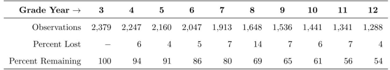
6.11 Coefficientβ1y Efficiency Gains forModel CRelative toModel I, by Specification 40 6.12 Coefficientβ2y Efficiency Gains forModel CRelative toModel I, by Specification 41 6.13 Coefficientβ1yEfficiency Gains forModel CRelative toModel E, by Specification 42 6.14 Coefficientβ2yEfficiency Gains forModel CRelative toModel E, by Specification 42 7.1 Available Data, by Grade Year . . . 46
7.2 Data Application Sample Size, by Grade Year . . . 47
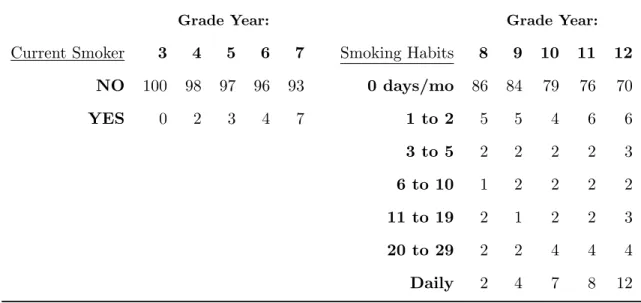
7.3 Reported Smoking Habits, Percent of Sample by Grade . . . 48
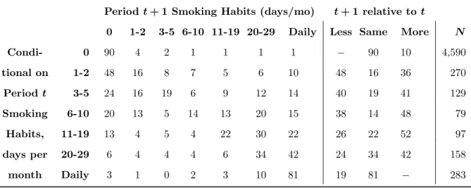
7.4 Smoking Transitions, Conditional on Lagged Use, Percent of Sample (Grades 8-12) 49 7.5 Attitudinal Response Variables Included in the Data Application . . . 50
7.6 Child’s Characteristics: Initial Sample . . . 52
7.7 Parent and Household Characteristics: Initial Sample . . . 53
7.8 Weight Status Dynamics, Percent of Sample . . . 55
7.9 Cotinine Level, Conditional on Smoking Habits, Percent of Sample (Grade 9) . . 56
7.10 Discrepancy in Responses . . . 57
8.1 Model IEstimated Latent-Factor Distribution . . . 59
8.2 Model EEstimated Latent-Factor Distribution . . . 59
8.3 Model C Estimated Latent-Factor Distribution . . . 60
8.4 Difference Between Observed and Predicted Smoking Outcome Means, by Year . 64 A.1 Model I: Observed Outcomes and Predicted Probabilities, Sample Means, by Year . . . 73
A.2 Model E: Observed Outcomes and Predicted Probabilities, Sample Means, by Year . . . 73
A.3 Model C: Observed Outcomes and Predicted Probabilities, Sample Means, by Year . . . 74
A.4 Model I,Model E, andModel CEstimated Response Parameters, Dependent Variable: Smoking . . . 76
A.5 Model C Estimated Parameters for Outcomes Att1 and Att2 . . . 79
A.6 Model C Estimated Parameters for Outcomes Att2 and Att3 . . . 81
A.7 Model C Estimated Parameters for Outcome Att4 and Attrition . . . 83
A.8 Model Iand Model EEstimated Attrition Parameters . . . 85
List of Figures
6.1 Distribution of latent factorλ . . . 23
6.2 Population Frequencies: Total Purchases Per Individual (P tyit), by Latent-Factor Distribution . . . 27
7.1 Household Composition: Birth Order . . . 51
7.2 Household Composition: Number of Siblings . . . 51
7.3 Cigarette Prices by Grade Year . . . 52
7.4 Weight Status, by Grade Year . . . 54
7.5 “Right now I look like ” . . . 57
8.1 Difference Between Observed and Predicted Smoking Outcome Means, by Grade Year . . . 63
8.2 Difference Between Observed and Predicted, with Confidence Intervals . . . 64
8.3 Estimated Marginal Effects: Parent Smoking Habits and Child Race, Sample Means, by Grade . . . 66
8.4 Difference Between Predicted Sample Average Smoking Behavior c Pr (Smoke|Abstain from smoking before 8th grade)−cPr (Smoke) . . . 67
Chapter 1
Introduction
For any empirical application, the researcher’s ability to quantify the determinants of an indi-vidual’s behavior is limited by the contents of the data, which generally consist of responses to objective questions. While this information describes the individual’s observed sociodemo-graphic and environmental characteristics, we might find ourselves wondering to what extent her demand for goods and services is influenced byintangiblepersonal characteristics: Did the individual’s mood affect her decision? How forward looking is she? How does she form expecta-tions over future outcomes that result from this decision? Typically, when these concerns enter our discussions, we acknowledge that these unobserved factors affect the outcome, regret that these data are not available, relegate their effects to the error component, and proceed with an assumption about the error term. But is there a better way to account for this unobserved heterogeneity?
It is becoming more common for surveys to include attitudinal questions that correspond to specific psychological traits. The participant’s subjective responses can give the researcher an idea of the individual’s mental state,1 locus of control,2 and opinions/beliefs,3 to name a few. However, it is not clear how these subjective reports of one’s well being might enter a standard model of economic decision making. In this paper, I construct a theoretical model to examine
1For example, measures of depression, stress, and anxiety are collected in the National Longitudinal
Study of Youth and Add Health studies.
2For example, the Panel Study of Income Dynamics and the National Longitudinal Survey datasets
record descriptions of participants’ perceptions of the extent to which they can control events that affect them.
3For example, marketing surveys ask consumers about their attitudes towards a product or a
the connection between attitudinal responses (r) and purchasing decisions (y). Ultimately, I conclude that the same exogenous characteristics and unobserved factors simultaneously affect both observed outcomes, and I derive a set of equations that, when jointly estimated, describes the significant determinants of the demand for goodyand the production of attitudinal response r. The econometric specification accounts for observed and unobserved sources of correlation by including the same covariates in each equation and estimating the distribution of common unobserved factors across equations.
I use econometric theory and Monte Carlo simulations to explore the benefits of my esti-mation strategy. Relative to other specifications introduced later in the paper, the standard errors for all response parameters are more efficient when the outcome y and the attitudinal response r are jointly estimated. Furthermore, I show that the efficiency gain grows as the correlation among latent factors strengthens. To support this theory, I conduct a Monte Carlo experiment that measures the efficiency gains under several different data and error generating processes. Data from the National Heart, Lung, and Blood Institute Growth and Health Study (NGHS), a longitudinal survey of individuals that features a rich set of attitudinal questions, are used in an empirical application of the econometric and behavioral theory described in this paper. Because the survey provides an extensive history of each participant’s smoking habits, the data application examines adolescent cigarette use. In this data application, the jointly-estimated model generates more accurate predictions of smoking behavior compared to some commonly-used specifications.
Chapter 2
Background and Contribution
This research draws from three topics in the literature: the use of attitudinal data in estima-tion, the role of unobserved heterogeneity, and the prediction of adolescent drug use. Having provided a brief literature review on each topic, I describe how previous research influences the structure of the empirical model, which is explained in further detail in Chapter 5.
2.1 The Use of Attitudinal Data
McFadden (1986) provided early support for using attitudinal data in estimation of eco-nomic relationships. He considers a scenario in which the researcher has information on the product’s characteristics, the individual’s purchasing decision, and the individual’s responses to attitudinal statements. These variables comprise a theoretical model in which unobserved personal characteristics interact with product attributes in the utility function to affect an individual’s purchasing decision. The unobserved characteristics simultaneously influence the individual’s responses to attitudinal questions. McFadden posits that jointly estimating pur-chasing decisions and attitudinal outcomes will produce more efficient parameter estimates. However, McFadden did not test this claim with an empirical application. My research builds on McFadden’s theoretical model to confirm the efficiency gain hypothesis.
the individual’s weight status, thoughts on dieting, depression, and behavioral conduct as ex-planatory variables. They find significant relationships between these subjective responses and smoking initiation. However, as the central idea of my paper, I claim that these results might suffer from two types of bias: reverse causality and simultaneity. For example, there might exist reverse causality between smoking and dieting because one might contribute to the other or simultaneity between smoking and behavioral conduct because peer pressure, an unobserved factor, might simultaneously affect both outcomes. The authors acknowledge the endogeneity bias but lack strong instruments to perform a two stage regression.
Boxall and Adamowicz (2002) use attitudinal data to explain campsite decisions. The data include responses based on a 5-point Likert scale that ranges from “Strongly Disagree” to “Strongly Agree.” For example, when given the statement “I go camping to relieve my ten-sions,” the respondent may “Disagree,” “Neither Disagree or Agree,” etc. The authors regress a recreationist’s campsite decision on the observable characteristics of each park, such as the user fee, the campsite type, and the campsite’s level of development. They incorporate unob-served heterogeneity with a latent-segmentation model, in which the marginal effects of campsite characteristics are homogeneous among individuals in a particular segment but different across segments. An individual’s responses to attitudinal statements (Pi) and demographic charac-teristics (Xi) influence her estimated latent-segment membership, and individuals belonging to latent segmentµk have taste parameters αk over campsite characteristics Zc. That is,
Pr (choicei =c;α) = X
k
Pr(µ=µk|Pi, Xi)∗Pr (choicei=c;αk|Zc, µ=µk). (2.1)
As a rebuttal to the previous paper, Morey et al. (2006) claim that the model (2.1) is mis-specified, as it improperly incorporates unobserved heterogeneity by modeling latent-segment membership backwards. Morey et al. state that using attitudinal data to explain membership into a particular segment is not appropriate, as they instead “assume that [segment] membership is exogenous and that the probability of giving a particular level of response to an attitudinal question is a function of one’s [segment].” To incorporate this intuition, the authors jointly model attitudinal responses with the demand equation and allow the unobserved heterogeneity to be correlated across equations. This specification expresses the idea that individuals from
the same segment answer questions similarly, and not that individuals who happen to answer questions in the same manner must belong to the same segment.
As an empirical application for this 2006 publication, Morey et al. (2011) jointly estimate anglers’ stated preferences among fishing grounds and their responses to attitudinal questions describing how bothered the anglers are by fish consumption advisories, how much they agree with particular “willingness-to-pay” statements, and how important certain fishing site at-tributes are to them. Their study offered anglers a choice set of hypothetical fishing grounds and recorded their stated preferences. The authors estimate a choice-only model and a joint choice-attitude model to show that the inclusion of attitudinal data does have an impact on the parameters of the choice probabilities, the parameters of the group membership probabilities, and the optimal number of latent groups to include in the final specification. Most importantly, the authors conclude that the joint model is small-sample more efficient than the choice-only model; the standard errors of the choice probability parameters are significantly smaller in the joint model. My research adds to their efforts by providing a theoretical motivation for includ-ing attitudinal responses, analyzinclud-ing the econometric properties of the joint model, and usinclud-ing revealed preference data from a longitudinal survey.
Conti et al. (2010) employ attitudinal data to analyze the impact of childhood cognitive ability and psychosocial traits on later-in-life outcomes. The data contain measures related to the individual’s academic ability, behavioral development, locus of control, and self-esteem at age ten and information on her education, health, and wage outcomes twenty years later.1 The authors jointly estimate 126 psychometric measurements, one education decision, six health outcomes, and two wage equations, using nine explanatory variables as covariates (xi) and ten latent factors (fi) to represent unobserved heterogeneity. The specification for the model is:
yi 135×1
= β
135×9
× xi
9×1
+ α
135×10
× fi
10×1
+ i 135×1
.
(2.2)
Each latent factor is assumed to be normally distributed. Conditional on the covariates, the latent factors serve as the only source of unobserved correlation between the late-life outcomes
1Conti et al. (2010) use data from the 1970 British Cohort Study. All participants were born in 1970.
and these attitudinal data. The results report statistically significant parameter estimates for
b
α, suggesting that the correlation among unobserved factors that influence attitudinal and objective outcomes is substantial. While this specification is based on the same reasoning as the model presented in Chapter 5 of my paper, the authors do not focus on efficiency gains. In addition, my model relaxes the assumption of normality for the latent factors.
2.2 Assumptions About Unobserved Heterogeneity
Imposing a distributional assumption on the error terms is a convenient way to account for unobserved heterogeneity. However, Heckman and Singer (1984) demonstrate that an incorrect assumption could lead to biased parameters. Instead, the authors describe a semi-parametric specification that does not impose any distributional assumptions on the structure of unobserved heterogeneity. In an exploratory paper, Chintagunta, et al. (1991) compare several specifica-tions of unobserved heterogeneity to the approach developed by Heckman and Singer (1984).2 They use longitudinal data on household saltine cracker purchases to investigate consumers’ heterogeneous brand preferences and conclude that the specified structure of heterogeneity plays an important role in determining the model’s accuracy. Overall, the semi-parametric ap-proach achieves the best model fit, as it generates more accurate predictions and outperforms alternative specifications on likelihood ratio tests.
Mroz and Guilkey (1995) and Mroz (1999) construct a Discrete-Factor Random Effects (DFRE) model that estimates the correlation across outcomes in a jointly-estimated set of equations. Like Heckman and Singer, the model approximates a discrete distribution for the unobserved heterogeneity by estimating the locations and probabilities for a finite number of mass points. As an extension, this DFRE model controls for both permanent and time-varying heterogeneity among the sample. Due to its flexibility in jointly modeling multiple outcomes, I use the DFRE estimation strategy for the Monte Carlo simulations (Chapter 6.2) and the empirical specification (Chapters 5 and 8) in this paper.
2The authors compare the semi-parametric model to specifications that incorporate heterogeneity
through previous purchasing behavior, heterogeneous response parameters, gamma-distributed latent factors, and normally-distributed latent factors.
2.3 Models of Smoking Behavior
The dangers of developing smoking addictions at an early age have been widely publicized. Consequently, many health economists have conducted extensive research on the determinants of drug use among adolescents. During the 1990’s, many state governments increased taxes on cigarettes in an attempt to discourage smoking initiation among adolescents. To measure the policy’s effectiveness, DeCicca et al. (2002) estimate price elasticities resulting from the tax changes using the 1988-1992 National Education Longitudinal Study (NELS) dataset. The authors do not control for previous cigarette use as they limit the sample to individuals who are not smokers in the baseline year, but they do estimate a first-difference model to eliminate any permanent unobserved heterogeneity. With onset of smoking between eighth and twelfth grades as the dependent variable, their results suggest that the change in cigarette tax did not have a significant effect on smoking initiation. Instead, demographics, other state laws, and academic performance proved to be the significant influences on smoking behavior.
With the same NELS dataset, Gilleskie and Strumpf (2005) revisit the question using a model that includes previous period cigarette use. They add a time-invariant individual het-erogeneity term via random effects to eliminate the endogeneity bias between consumption and lagged consumption resulting from permanent unobserved factors. The authors find small yet significant effects of previous smoking behavior in their unbiased coefficient estimates. Ad-ditionally, after incorporating these variables, estimates show that the tax increases were in-deed effective in discouraging smoking initiation. They stress the importance of controlling for lagged behavior on top of permanent latent factors since “persistence cannot be fully explained by unobserved heterogeneity,” as shown by the significant coefficients on lagged cigarette use intensities.
Arcidiacono et al. (2007) use data from the Health and Retirement Study to understand smoking and drinking behavior. Their structural approach relaxes the traditional assumption of a sample-wide discount factor (β). As a baseline, the authors construct a latent-segment model with a homogeneousβ, which estimates an annual discount factor of 0.91. The next model allows the discount factor to vary based on the individual’s latent segment. The unconstrained model yields estimates between 0.69 and 0.99 for different segments of the sample. This result suggests
that an individual’s discount factor is a significant source of unobserved heterogeneity in regards to decisions about cigarette and alcohol use. Their empirical findings provide motivation for the implications of the theoretical model of behavior in Chapter 3.
2.4 Contribution to the Literature
Overall, my paper expands upon the works of Morey et al. (2006) and Conti et al. (WP, 2010) by conducting a thorough investigation of the role of attitudinal data in estimation. First, my paper builds an economic model of behavior to motivate the inclusion of attitudinal data as an outcome rather than an exogenous variable within the empirical specification. Second, I provide an econometric proof to demonstrate how the jointly-estimated model improves the efficiency of the estimated parameters. Third, I construct a Monte Carlo experiment to validate this conclusion for small sample sizes. Finally, while the other papers only provide results from the jointly-estimated model, the data application in my paper compares the prediction accuracy of this specification against other commonly-used specifications.
Chapter 3
Theoretical Model of Consumer Behavior
Ultimately, this paper shows that the strength of the correlation among the unobserved factors that affect both the decision of interest (y) and attitudinal response (r) drives the efficiency gains for the model that jointly estimatesy andr. The behavioral theory supplement to this paper, summarized here, demonstrates how three such unobserved factors representing the individual’strueunderlying preferences−the structural parametersµ(a preference shifter),
β (the discount factor), andα(a subjective expectations parameter)−simultaneously impact the decision making process for y and the production of attitudinal response r.
In the theoretical model of consumer behavior, the inputs to the contemporaneous utility function for individual iin time periodt are:
yit Outcome/decision of interest
cit Aggregate consumption good (excluding yit) Xit Exogenous factors
Yit Vector of variables describing an individual’s decision history up to timet
Sit Other information that impacts the individual’s decisionyit and is affected by past decisions(treated as a state variable)
it Idiosyncratic utility shock
example from my data application, I would claim that smoking cigarettes (yit>0) becomes less desirable when the individual has trouble breathing (Sit =adverse health shock). Additionally, choosing to smoke more frequently can increase the probability of experiencing an adverse health shock in the next period.1 In this model, the consumer does not know with certainty how her period t decision (yit) affects her state realization next period (Sit+1). She forms a subjective expectation, represented byα, to approximate the impact ofyit on Sit+1. Without loss of generality, there are two possible states: Sit∈ {0,1}.
The individual’s previous history of consumption represents another dynamic aspect of the decision making process. As an example, it has been shown that prolonged use of cigarettes is partly explained by habit formation. For this setting, variables for experience, duration, and cessation describe the history of previous decisions, Yit.
3.1 Utility Function and Value Function
The contemporaneous utility function is given by:
USit(y
it, cit;µ, Xit, Yit, yit). (3.1)
The individual spends her income on yit and general consumption goods cit. The primitive parameter µ represents a preference shifter for consumption of yit, and I assume that the marginal utility of consuming good y is a function of µ, among several other factors. In traditional economic models, µ might enter the utility function as a risk aversion parameter or as a taste parameter. In this dynamic optimization problem, the consumer’s current period decisions affect future realizations of history Yit and state Sit variables. The individual is forward looking in that she takes into account the discounted expected utility from future time periods when making a decision for the current period. The discount factor β, which describes how the individual values future streams of utility, is another behavioral primitive of the optimization problem. For each period, the individual considers the contemporaneous
1Other decision-state pairs exhibiting this relationship include weight loss food consumption and
weight, cleaning supply usage and household cleanliness, and dietary supplement/steroid usage and strength.
utility from that period’s decision and the effects of this decision on the discounted present value of future utility flows.
I assume that, in period t, the individual does not know the marginal effect of her decision yiton next period’s state realizationSit+1 and must generate a subjective expectation over this parameter. Her subjective-expectations operator, α, represents the individual’s belief of how her decision impacts future state transitions and enters the expected state transition probabil-ities π0it(α, yit, Xit, Yit) = E[Pr (Sit+1= 0)] and π1it(α, yit, Xit, Yit) = E[Pr (Sit+1 = 1)]. Her conditional (on next period’s state realization Sit+1) maximum expected future lifetime utili-ties are represented by V0(•) and V1(•). Conditional on the current period state realization Sit=S, the value function for alternative yit=y is given by:
VySµ,β,α, Xit, Yit, ySit
=USit=S(y
it=y,[Iit−pty] ;µ, Xit, Yit, ySit )
+β∗π1(α, yit, Xit, Yit)∗V1(µ,β,α, Xit+1, Yit+1)
+β∗π0(α, yit, Xit, Yit)∗V0(µ,β,α, Xit+1, Yit+1).
(3.2)
Here, general consumption is inferred from incomeIitand the price ofyit,pt, ascit =Iit−ptyit. In summary, the relevant primitives of the optimization problem that will drive the unob-served correlation across equations enter the model through the:
• Preference shifters,µ
• Time preference parameter (discount factor),β
• Subjective expectations over future states,α.
3.2 Optimal Decision Rules for Decision yit
Using the value function specification in (3.2), the individual chooses at each period t the alternative that maximizes her remaining lifetime utility. The discrete-choice framework uses choice probabilities to describe the probability that outcome yit=y occurs. That is,
Pr (yit=y|µ,β,α, Xit, Yit, Sit =S, it)
= PrVySµ,β,α, Xit, Yit, ySit
≥Vy˜Sµ,β,α, Xit, Yit, ySit˜
,∀y˜6=y.
(3.3)
Clearly, the choice probabilities are functions of primitive parameters µ, β, and α because they define the optimization problem. A more rigorous proof in the Appendix derives the optimality conditions to show this relationship more explicitly.
3.3 Production of Attitudinal Responses rit
Contrary to decisions yit, attitudinal responses are outcomes that are influenced by sev-eral factors of the individual’s environment. She, herself, does not choose her attitudes; she merely reports the outcome that occurred. Similar to the value function of equation (3.3), the attitudinal index function A(•) describes how the individual’s response to an attitudinal question is produced. The probability of giving a particular response is a function of personal characteristics, primitive parameters, and other unobserved factors. That is,
Pr (rit=r|µ,β,α, Xit, Yit, Sit=S, ηit)
= Pr ASr µ,β,α, Xit, Yit, ηitrS
≥AS˜r µ,β,α, Xit, Yit, ηit˜rS
,∀r˜6=r
.
(3.4)
The factors that influence responses to attitudinal questions can be grouped into four categories:
1. Exogenous characteristics Xit, history vector Yit, and state Sit explain system-atic differences in the way individuals generate attitudinal responses.
2. In deciding which attitudinal response questions are relevant to the demand behavior of interest, I select only those questions that can conceivably be affected by primitive parameters such as preference shifter µ, the discount factor β, and the subjective-expectations operator α.
3. No survey can capture everything that affects a person’s behavior; there are several un-observed factors and events that influence the individual’s attitudinal responses on the survey.
4. Attitudes and feelings are intangible and difficult for the respondent to quantify on a survey form. Reporting opinions based on a 5-point Likert scale presents the possibility of measurement errorin reporting her true beliefs.
Factors described in categories 3 and 4 comprise the composite error term ηit. Factors de-scribed in categories 1, 2, and 3 might simultaneously influence the outcomeyit. The important latent correlation between yit and rit that justifies the joint estimation proposed by this paper is driven by factors found in categories 2 and 3, as ultimately these data will be unobserved to the econometrician in the empirical model. The implications of this effect are explained in greater detail in the next section.
Chapter 4
Implications for the Empirical Model
For the data application, I do not include an endogenous state variable in order to keep the model more tractable.1 Thus, the model comprises equations (3.3) and (3.4):
Pr (yit=y|µ,β,α, Xit, Yit, it)
= PrVy(µ,β,α, Xit, Yit, yit)≥Vy˜
µ,β,α, Xit, Yit, yit˜
,∀y˜6=y
Pr (rit=r|µ,β,α, Xit, Yit, ηit)
= Pr Ar(µ,β,α, Xit, Yit, ηitr)≥A˜r µ,β,α, Xit, Yit, ηrit˜
,∀ ˜r6=r
(4.1)
I use Taylor Series approximations to the alternative-specific value and attitudinal index func-tions to obtain reduced form expressions for the demand function foryitand production function forrit. The following outcome probabilities represent the linear approximations of functionsVy and Ar, in which {γ, φ} and {ωit, τit} are the coefficients and error terms of the Taylor Series approximations:
Pr (yit=y|µ,β,α, Xit, Yit, it)
= PrVy(µ,β,α, Xit, Yit, yit)≥Vy˜
µ,β,α, Xit, Yit, yit˜
,∀y˜6=y
≈PrXitγXy +YitγYy +ω y
it≥XitγXy˜ +YitγYy˜ +ω
˜
y
it,∀y˜6=y
= Prωyit−ωyit˜ ≥Xit
γXy˜ −γXy+Yit
γYy˜ −γyY,∀y˜6=y
≡Pr (yit=y|Xit, Yit)
(4.2)
1In theAppendix, I outline a specification that estimates the transition equation for an endogenous
Pr (rit=r|µ,β,α, Xit, Yit, ηit)
= Pr Ar(µ,β,α, Xit, Yit, ηrit)≥Ar˜ µ,β,α, Xit, Yit, ηit˜r
,∀r˜6=r
≈Pr XitφrX+YitφrY +τ r
it≥Xitφ˜rX+YitφrY˜ +τ
˜
r
it,∀˜r6=r
= Pr τitr−τitr˜≥Xit φrX˜ −φ r X
+Yit φ˜rY −φ r Y
,∀ ˜r6=r
≡Pr (rit=r|Xit, Yit) .
(4.3)
The approximation approach is common among empirical economic research because it reduces the computation time while retaining the ability to predict outcomes and produce policy sim-ulations. This method, however, does not recover the structural parameters that shape an individual’s decision making problem. For instance, in equations (4.2) and (4.3), the total ef-fects of the explanatory variables on the outcome probabilities are aggregated into the response parameter vectors {γX, γY} and {φX, φY}, which are functions of the underlying structural parameters µ,β, andα.
The theoretical model in Chapter 3 suggests that error termsωit andτitare correlated, and the econometric analysis discussed later in Chapter 6 shows that jointly estimating outcomes yitandritproduces more efficient parameter estimates. A random effects model accommodates these considerations by incorporating latent factors λandνtinto each equation to account for the shared unobserved heterogeneity. The error terms are decomposed into three components:
ωyit τr
it
=λy+νty+ξity =λr+νr
t +ζitr
(4.4)
Here, E[λy, λr]=6 {0,0}, E[νty, νtr]6={0,0}, and ξit and ζit areiid serially uncorrelated errors. An assumption that the idiosyncratic shocks ξit and ζit follow independent GEV distributions creates a closed form expression for the choice probabilities, given by:
Pr (yit=y|Xit, Yit, λy, νty) =
exp (Xitγ y X+Yitγ
y
Y +λ
y+νy t)
P
˜
yexp
Xitγ
˜
y X+Yitγ
˜
y
Y +λy˜+ν
˜
y t
(4.5)
Pr (rit=r|Xit, Yit, λr, νtr) =
exp (XitφrX+YitφrY +λr+νtr)
P
˜
rexp XitφrX˜ +YitφYr˜ +λr˜+νt˜r
(4.6)
Further details on estimation are explained in Chapter 5.
4.1 Comparison: Attitudinal Responses are Treated as Exogenous Variables
In the recent economic literature, many empirical specifications do include data on the individual’s attitudes. However, attitudinal responses are often treated as explanatory variables in the choice probabilities for yit, where
Pr (yit=y|Xit, Yit, rit)
= Prωity −ωity˜ ≥Xit
γyX˜ −γXy+Yit
γYy˜−γYy+rit γry˜−γry
,∀y˜6=y.
(4.7)
Here,ritenters the problem as an exogenous right-hand-side variable. The conclusions from the theoretical model of behavior in Chapter 3.3 contradict this assumption because unobserved fac-torsωitsimultaneously affect attitudinal responserit. A biased estimate for response parameter γr and inefficient estimates for all other parameters result from this specification. Furthermore, significant multicollinearity between the endogenous response variableritand other explanatory variables could bias response parameters γX and γY as well. Incorporating latent factors does not eliminate the endogeneity bias since the initial specification (4.7) assumes independence between the explanatory variables andallcomponents of error termωit.
Attitudinal data have also been used to control for unobserved heterogeneity in latent-segment models (Boxall and Adamowicz, 2002). The model estimates response parameters for different segments of the sample, and each individual in the sample is placed into a segment based on her attitudinal responses. However, this model is misspecified as it imposes an incor-rect diincor-rection of causality. Instead, my model assumes that all individuals from a particular segment respond to attitudinal questions in the same manner, with an idiosyncratic shock to explain the differences, which emphasizes that the individual’s type is the exogenous personality trait that influences her responses on the survey.
Chapter 5
Empirical Specification
In the data application, the preferred model jointly estimates the choice probability for y (4.5) with the response probabilities forQattitudinal questions of the form (4.6). The possible response categories for yit are {0, . . . ,Y} and for attitudinal question rq are {0, . . . ,Rq}. For identification, the model normalizes parameters with respect to alternative 0.1 The likelihood contribution of the period t outcomes for individual i, conditional on latent factors λand νt, equals:
`(yit,Rit|zit, λ, νt; Θ)
= Y
Q
y=0
Pr (yit=y|zit, λ, νt)1
(yit=y)∗ Q
Q
q=1 Rq
Q
rq=0
Pr (rqit=rq|zit, λ, νt)1
(rqit=r).
(5.1)
For brevity, I represent attitudinal responses{r1it, . . . , rQit} with vector Rit, condense charac-teristics{Xit, Yit}intozit, consolidate response parameters{γ, φ}into Θ, and index attitudinal questions by q. The Discrete-Factor Random Effects (DFRE) model approximates the latent-factor distributions by estimating K mass points for the vector λ and L mass points for the vectorνt, and the dimensional size of each mass point equals the number of equation-alternative pairs in the model. This method associates probabilities{pk}Kk=1 to mass points{λk}Kk=1 and probabilities{ql}Ll=1 to mass points{νtl}Ll=1. For illustration, the latent factor parameterization for mass pointλ1 is summarized by
λ1 ={λy11 , . . . , λ yY 1
| {z }
equation fory, alt’s 1,...,Y
, λ111 , . . . , λ1R1
1
| {z }
equation forr1,
alt’s 1,...,R1
, . . . , λQ11 , . . . , λQR1 Q
| {z }
equation forrQ,
alt’s 1,...,RQ
} {p1}= Pr (λ=λ1). (5.2)
1For alternative 0, Pr (y
it= 0|Xit, Yit, λ, νt) = 1−ΣyY=1Pr (yit=y|Xit, Yit, λ, νt) and likewise for
The unconditional likelihood contribution for individualibecomes:
L{yit,Rit}Tt=1| {zit}Tt=1; Θ,p,q
= K X
k=1
pk
T Y
t=1 L X
l=1
ql∗`(yit,Rit|zit, λk, νtl; Θ). (5.3)
Aggregating across all individuals in the sample creates the empirical likelihood function,
L(y,R|Z; Θ,p,q) = N Y
i=1
L{yit,Rit}Tt=1| {zit}Tt=1; Θ,p,q
. (5.4)
Chapter 6
Econometric Motivation
6.1 Fisher Information Matrix
I examine a case of two binary random variables, y ∈ {1,2} and r ∈ {1,2}, in which y is the outcome of interest and r is the response to an attitudinal question.1 Diagonal elements of the inverse of the Fisher information matrix are used to find the asymptotic variance of the parameters in the choice probabilities. Hence, I present the Fisher information matrices for two logit models in order to show that the standard errors of the estimated parameters are smaller when the unobserved factors are allowed to be Correlated across equations in Model C than when they are assumed to be Independent in Model I. Ultimately, the degree of correlation between the unobserved factors that affectyand the unobserved factors that affectrdetermines the efficiency gains in Model CoverModel I.
• Model Cjointly models the outcome, attitudinal response, and correlation, in which the joint probability, Pr y=j, r=k|X;βC
, cannot be separated into marginal probabilities without modeling the correlation coefficient.
• Model I assumes conditional independence between the outcome and attitudinal re-sponse, such that:
Pr y=j, r=k|X;βI= Pr y=j|X;βyI∗Pr r=k|X;βrI.
Due to the independence assumption inModel I, simply estimating Pr y|X;βyI by itself will produce an identical point estimate and variance for response parameter βI
y. Thus, Model I is equivalent to a standard logit specification that estimates only the choice probability for y, which is the case when attitudinal information is either ignored or not collected. ForModel C, a bivariate logistic model accurately captures the relationship between two correlated binary random variables (y, r).2 For outcome y, outcomer, and a set of explanatory variablesX, the parameterizations for the log-odds ratios of the jointly-estimated model are:
1McCullagh and Nelder (1989) explain how this case can easily be extended to accommodate
cate-gorical variables with more than two alternatives.
2Ultimately, I use a logistic model in my empirical model. A similar proof, used in Meng and Schmidt
(1985), derives the Fisher information matrix for a bivariate probit model, which shows the same results as those presented here.
log
Pr(y=1|X) Pr(y=2|X)
=βyCX,
log
Pr(r=1|X) Pr(r=2|X)
=βrCX,
and log
Pr(y=1,r=1|X)∗Pr(y=2,r=2|X) Pr(y=1,r=2|X)∗Pr(y=2,r=1|X)
=βyrC.
(6.1)
The first two equations estimate response parameters βyC and βrC while the third equation estimates the correlation coefficient,βyrC, between the error terms.
My primary focus turns to the asymptotic properties of βy, the response parameter for X on the outcome of interest, for each model. The proof in McCullagh and Nelder (1989) shows that both estimators βyC and βyI are asymptotically unbiased, but the estimator βyC is more efficient. To compare the variances ofβyC andβyI, the econometrician only needs to analyze the second principal minor of the Fisher information matrix for Model C and the first principal minor of the matrix forModel I:3
F2ndM(C) =
βyC βrC
βyC βrC
X0diag
nV y
∆ o
X
X0diag∆π
∆ X
X0diag∆π
∆ X
X0diagVr
∆ X
.
(6.2)
F1stM(I) =
βyI
βyI
X0diag{Vy}X
(6.3)
The termsVy,Vr,Vyr, ∆, and ∆π represent functions of joint probabilities Pr (y=j, r=k|X), and the operator diag{•} transforms the N ×1 vector in brackets into a diagonal matrix of rank N.
Equations (6.2) and (6.3) show that the value of ∆ plays an important role in determining the efficiency gains of Model Cover Model I. When the error terms are independent, then ∆ = 1 and ∆π = 0. Under this condition, the variances of βyC and βyI will be identical, and the jointly-estimated system of outcomes provides no benefits. However, if the error terms are
3Some rows and columns of each matrix can be ignored as they do not affect the variance of β y,
found in the inverse Fisher information matrices.
correlated, then ∆< 1, and the (1,1) element of FM(C) is greaterthan the (1,1) element of FM(I). When the matrices are inverted to attain the variances, this relationship is reversed, which means the variance of βyC will besmaller than the variance ofβyI.
6.2 Monte Carlo Simulations
This Monte Carlo experiment uses a simple data generating process to compare five em-pirical models, ultimately showing that the jointly-estimated model improves the small-sample accuracy and efficiency of the estimated parameters when significant correlation exists among the unobserved factors that influence the outcome y and the attitudinal response r. To mea-sure these gains under different environments, 96 unique data specifications are generated by specifying the number of individuals, number of time periods, latent-factor distribution, and strength of correlation between error terms across outcomes.4 The eight individual-period pairs include either 500 or 1,000 individuals for 1, 3, 5, or 10 time periods.
Table 6.1: Monte Carlo Specification Options: Individual-Period Pairs
(N, T) # Periods = 1 # Periods = 3 # Periods = 5 # Periods = 10 # Individuals = 500 (500,1) (500,3) (500,10) (500,10) # Individuals = 1000 (1000,1) (1000,3) (1000,10) (1000,10)
6.2.1 Unobserved Heterogeneity
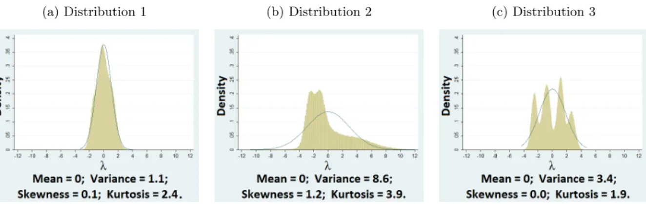
The econometric theory supplement shows that the efficiency gain increases as the correla-tion among error terms grows stronger. To test this theory, the Monte Carlo data generating processes allow for differences in the error correlation structure. One time-invariant latent fac-tor enters the data generating processes for outcomes y and r. To relax the assumption that the latent terms must follow a conventional distribution, each individual’s latent factor is inde-pendently drawn from a mixture of normal distributions. For robustness, three such mixture distributions, shown in Figure 6.1, are considered. Distribution 1 is very close to the standard normal density. Distribution 2 is skewed to the left and has a heavy right tail. Distribution 3
4There are two options for the number of individuals, four options for the number of time periods,
three latent-factor distributions, and four options for the factor loading on the latent factor.
contains four distinct high-density areas, but its variance is smaller than that of Distribution 2. A normal-density bell curve overlays each graph in Figure 6.1 for comparison.
Figure 6.1: Distribution of latent factorλ
(a) Distribution 1 (b) Distribution 2 (c) Distribution 3
In each outcome’s data generating process (DGP), the composite error term is composed of an additional independently- and identically-distributed (iid) generalized extreme value (GEV) disturbance (explained in the following section) and the composite latent-factor term. The latent termλi influences both outcomes and enters both DGP’s additively. The magnitude of latent factor λi in the DGP for outcome y is constant across specifications. This magnitude in the DGP for outcome r, represented by ρr, varies from zero to 0.9 (ρr ={0,0.3,0.6,0.9}). There is no correlation across error terms for specifications in whichρr = 0, but this correlation strengthens asρrincreases. This relationship is illustrated in the DGP summary of the following section.
6.2.2 Data Generation for Longitudinal Specifications
An initial condition, yi0, is estimated for longitudinal specifications in which T > 1. Con-ditional on an exogenous characteristic (Wi0) and the latent factor (λi), dichotomous outcome yi0 follows an iid GEV distribution, which creates a closed-form expression for the outcome probabilities. For all outcomes, I construct a latent index, compute the logistic probability, and draw a random variable Ψ from a standard uniform distribution,U[0,1]. The model produces the outcomeyi0 = 1 if the logit probability exceeds random variable Ψ and the outcomeyi0 = 0 otherwise. The data generation process foryi0 is summarized by the following:
1. Draw Wi0∼ N(0,36) andλi from the specified distribution. 2. Construct latent indexyi0∗ =βy0
0 +β y0
1 Wi0+λi. 3. Draw Ψyi0 ∼U[0,1].
4. Generate outcome yi0 =1
exp(y∗ i0)
1+exp(y∗i0) ≥Ψ y i0
.
The outcomes in the remaining T −1 periods are generated through a similar process. To incorporate persistence in purchasing behavior, the previous period outcome yit−1 influences current period outcomeyit. As a result, an empirical specification that does not account for the serial autocorrelation caused by time-invariant latent factorλiwill produce a biased estimate for the marginal effect of yit−1 on yit. Previous period outcomes yit−1 and rit−1 are not included in the data generation process of current period attitudinal responses rit so that the model conforms to the assumptions of the theoretical model and empirical specification in this paper.5 A time-varying exogenous characteristic, Xit, influences both outcomes yit and rit. The entire data generating process is summarized below:
Wi0∼ N(0,36) and Xit∼ N(0,36) fort= 1, . . . , T −1.
λi is drawn from the specified latent-factor distribution.
Ψyi0,Ψyi1,Ψri1, . . . ,ΨiTy −1, and ΨriT−1 are drawn independently fromU[0,1].
yi0 =1
exp(y∗i0) 1+exp(y∗ i0)
≥Ψyi0
, wherey∗i0 =βy0
0 +β y0
1 Wi0+λi.
yit=1
exp(y∗ it)
1+exp(yit∗) ≥Ψ y it
, whereyit∗ =β0y+β1yyit−1+β2yXit+λi, fort= 1, . . . , T−1
rit=1
exp(r∗it)
1+exp(rit∗) ≥Ψ r it
, whererit∗ =β0r +β2rXit+ρrλi, fort= 1, . . . , T−1.
The coefficients of the model and distributions of exogenous characteristics are chosen so that latent factorλi does not overpower the influence of observed explanatory variables on outcomes y and r (explained in Section 6.2.4). For this Monte Carlo experiment, βy0
0 = 1, β y0
1 = −0.5, β0y = −1, βy1 = 0.75, β2y =−0.5, β0r = −1, and β2r = 0.5. For illustration, the following steps
5Results are available for a specification in which y
it−1 is also allowed to influencerit. These results
show no difference in model performance.
outline the data generation process for a specification in whichN = 500, T = 5, latent-factor distribution 2 is used, andρr= 0.9:
1. For 500 individuals, draw Wi0 ∼ N(0,36) andλi from latent-factor distribution 2.
2. Construct latent indexyi0∗ = 1−0.5Wi0+λi.
3. Draw Ψyi0 ∼U[0,1].
4. Generate outcome yi0 =1
exp(y∗i0) 1+exp(y∗ i0)
≥Ψyi0
.
5. Draw Xi1∼ N(0,36).
6. Construct latent indecesyi1∗ =−1 + 0.75yi0−0.5Xi1+λi andri1∗ =−1 + 0.5Xi1+ 0.9λi.
7. Draw Ψyi1 ∼U[0,1] and Ψri1∼U[0,1].
8. Generate outcomesyi1 =1
exp(y∗i1) 1+exp(y∗ i1)
≥Ψyi1
and ri1=1
exp(r∗i1) 1+exp(r∗ i1)
≥Ψri1
.
9. Repeat steps 5. through 8. for time periods 2, 3, and 4.
6.2.3 Data Generation for Cross-Sectional Specifications
For the cross-sectional specifications, only one outcome yi1 and one attitudinal responseri1 are generated for each individual. An initial condition is not estimated in these specifications. Instead, variable yi0 replaced by a normally-distributed exogenous variable, drawn indepen-dently of λi. Thus, for cross-sectional specifications, the parameters do not suffer from an autocorrelation bias and the latent factor simply adds noise to the estimation. The same coef-ficient, sample size, latent-factor distribution, and factor loading options from the longitudinal specifications are used for the cross-sectional specifications.6
6This data generating process is summarized by the following steps:
1. Drawyi0∼ N(0,16),Xi1∼ N(0,36), andλi from the specified distribution.
2. Construct latent indecesyi∗1=β0y+β1yyi0+β
y
2Xi1+λi andri∗1=βr0+β2rXi1+ρrλi.
3. Draw Ψyi1∼U[0,1] and Ψr
i1∼U[0,1]. 4. Generate outcomesyi1=1
exp(y∗i1) 1+exp(y∗
i1)
≥Ψyi1
andri1=1
exp(r∗i1) 1+exp(r∗
i1)
≥Ψri1
.
6.2.4 Monte Carlo Summary Statistics
The two exercises in Section 6.2.4 quantify the impact of the latent factors on the data generating process (DGP) for outcomesy and r in the Monte Carlo experiment. For brevity, I analyze only specifications that include 1,000 individuals for 10 time periods. The exercises are repeated 2,000 times, and I average across these iterations to generate summary statistics. In order to isolate the impact of latent factors on the outcomes, only one complete set of exogenous covariates {Xit, Wi0} and uniform random variables {Ψyit,Ψrit} is drawn and used repeatedly throughout the exercises. Conditional on this fixed set of data, the only remaining variables are the latent factor (drawn at random from the specified distribution for every individual in each repetition) and the factor loading parameter ρr, which varies by specification.
The parameters for the distribution of latent factorλiwere chosen such that the unobserved heterogeneity is not the dominant source of variation for outcome y. To verify this claim, the first exercise appeals to the time-invariant property of the latent factors. If, in the DGP, the impact of the time-invariant latent factors overpowers the influence of the time-varying exogenous characteristics, which is what I want to avoid, individuals will be very persistent in their purchasing behavior. Specifically, individuals who receive an extremely negative draw for latent factor λi will never purchase good y (Yi = {0,0, . . . ,0}), and those who receive an extremely positive draw will always purchase the good (Yi ={1,1, . . . ,1}). The frequency of total purchases (P
tyit) in time periodst= 1, . . . ,10 among the sample are displayed in Figure 6.2. As a baseline comparison, when I omit the latent factor from the DGP, goodyis purchased zero times or ten times over the ten time periods by only 1% of the Monte Carlo sample. Under latent-factor Distribution 3, 2% of the sample purchases goody in each period and 4% never purchases the good. For Distribution 1, which has a lower variance, 2% of the sample purchases the good either zero or ten times. For Distribution 2, which has a higher variance, this percentage increases to 15%. Thus, the influence of time-variant exogenous characteristics in the DGP is not overshadowed by the permanent unobserved heterogeneity. Figure 6.2e shows an undesirable dispersion of frequencies that results from increasing the variance of Distribution 2 by a factor of 10. This dramatically increases the probability of receiving an extremely high or low draw for λi. The frequency of persistent purchasing habits across time jumps to 88%,
suggesting that, in this extreme case, the individual’s time-invariant latent-factor draw largely dictates the outcome realization.7
Figure 6.2: Population Frequencies: Total Purchases Per Individual (P
tyit), by Latent-Factor Distribution
(a) Distribution 1 (b) Distribution 2 (c) Distribution 3
(d) Baseline, No Latent Factor (e) Extremely High Variance
An extremely high variance for
the distribution of latent factor
λi (Figure 6.2e) is undesirable
because the time-invariant latent
factor draw largely determines
outcomey.
The factor loading parameter ρr plays a significant role in the DGP for outcomer. Ceteris paribus, latent factor λi has no impact on r when ρr = 0. However, a positive value for ρr generates a positive correlation between λi and r, similar to the positive correlation between λi and y. Thus, an increase in the magnitude of ρr strengthens the correlation in the error terms of outcomes y and r. For this second exercise, all other parameters and variables are held constant to quantify the impact of factor loading ρr on the generated response r. The off-diagonal elements of Contingency Table 6.2 report the percentages of outcomes that switch from 0 to 1 or from 1 to 0 following a change in the magnitude of ρr. The largest shift in outcome realizations occurs under Distribution 2 when the magnitude ofρr increases from zero to 0.9; 20% of the outcomes change after the increase.
7An identical conclusion results from repeating the exercise for outcome runder all specified values
ofρr; the latent factor is not the dominant source of variation in the DGP for outcome r.
Table 6.2: Contingency Tables for Outcomer, by Magnitude of Factor Loading ρr
rtwhen rtwhen rt when
ρr= 0.3 ρr= 0.6 ρr= 0.9
0 1 0 1 0 1
Latent-Factor
rt whenρr= 0
0 60 2 0 58 3 0 57 5
Distribution 1 1 1 37 1 3 36 1 4 34
0 1 0 1 0 1
Latent-Factor
rt whenρr= 0
0 57 4 0 54 8 0 51 10
Distribution 2 1 4 35 1 7 31 1 10 29
0 1 0 1 0 1
Latent-Factor
rt whenρr= 0
0 59 3 0 56 6 0 53 8
Distribution 3 1 2 36 1 5 33 1 7 32
Off-diagonal elements represent the percent of outcomes affected by a change in the magnitude of ρr.
Summary statistics are reported in Tables 6.3 and 6.4. The penultimate row of Table 6.4 shows that the correlation across outcomes becomes more positive as factor loadingρrincreases. The last row of Table 6.4 reports the correlation coefficient between the composite error terms in the DGP fory and r, which each consist of the latent factor and GEV shock.
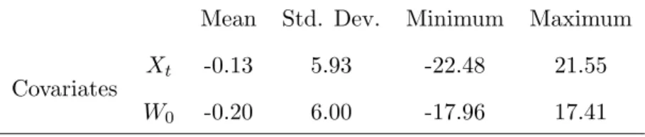
Table 6.3: Monte Carlo Summary Statistics: (N, T) = (1000,10)
Mean Std. Dev. Minimum Maximum
Covariates
Xt -0.13 5.93 -22.48 21.55 W0 -0.20 6.00 -17.96 17.41
6.2.5 Statistical Models Compared in the Estimation of the Monte Carlo
Experiment
To test the econometric theory in Section 6.1, I compare a Discrete-Factor Random Effects (DFRE) model that does not use attitudinal data (Model I) to a DFRE model that jointly estimates both observed outcomesy andr(Model C,the preferred model). I also compare the preferred model against other empirical methods found in the literature, including a standard logit model (Model L1), a logit model with attitudinal responses as explanatory variables (Model L2), and a DFRE model with attitudinal responses as explanatory variables (Model E). The Monte Carlo experiment simulates 500 repetitions for each of the 96 specifications. The latent factors used to generate the data are unobserved by the econometrician. The statistical models for longitudinal specifications are outlined below. For cross-sectional specifications, the initial condition equation in each model is omitted because only time periodt= 1 is estimated.
1. Model L1− Logit without Attitudinal Responses
lnPr(yi0=1)
Pr(yi0=0)
=βy0
0 +β y0
1 Wi0
ln
Pr(yit=1)
Pr(yit=0)
=β0y+β1yyit−1+β2yXit fort= 1, ..., T −1
(6.4)
2. Model L2− Logit with Attitudinal Responses as Explanatory Variables
ln
Pr(yi0=1)
Pr(yi0=0)
=βy0
0 +β y0
1 Wi0
ln
Pr(yit=1)
Pr(yit=0)
=β0y+β1yyit−1+β2yXit+βy3rit fort= 1, ..., T−1
(6.5)
3. Model I−DFRE, Logit
lnPr(yi0=1)
Pr(yi0=0)
=βy0
0 +β y0
1 Wi0+λy0 lnPr(yit=1)
Pr(yit=0)
=βy0 +β1yyit−1+βy2Xit+λy fort= 1, ..., T −1
(6.6)
4. Model E−DFRE, Logit with Attitudinal Responses as Explanatory Variables
lnPr(yi0=1)
Pr(yi0=0)
=βy0
0 +β y0
1 Wi0+λy0 ln
Pr(yit=1)
Pr(yit=0)
=βy0 +β1yyit−1+βy2Xit+β3yrit+λy fort= 1, ..., T−1
(6.7)
5. Model C−DFRE, Logit of Jointly-Estimated Outcomesyand Attitudinal Responsesr
ln
Pr(yi0=1)
Pr(yi0=0)
=βy0
0 +β y0
1 Wi0+λy0 ln
Pr(yit=1)
Pr(yit=0)
=βy0 +β1yyit−1+βy2Xit+λy fort= 1, ..., T −1
ln
Pr(rit=1)
Pr(rit=0)
=β0r+β1ryit−1+β2rXit+λr fort= 1, ..., T −1
(6.8)
Chapter 5 explained the DFRE estimation routine in detail. Briefly, taking Model C as an example, the DFRE method estimates several mass points of the form cλk=
n c
λy0
k ,λc y k,cλrk
o and assigns a probability to each mass point, in which pbk = Pr
λ=λck
. These parameters are used in the likelihood function to integrate over the distribution of the permanent unobserved heterogeneity. The Bayesian Information Criterion (BIC) is used to select the optimal number of mass points in each repetition.
6.2.6 Hypotheses
In longitudinal specifications, explanatory variableyit−1and dependent variableyitare both functions of latent factorλi. Models L1andL2do not address the serial autocorrelation, which should result in biased estimates for coefficientβcy
1. Models I,E, andC incorporate random effects to address the serial autocorrelation by estimating the distribution of the unobserved heterogeneity, which improves the accuracy of the estimated coefficients. For cross-sectional specifications, no estimated coefficients suffer from an endogeneity bias, but the latent factor λi still introduces a significant amount of noise to the model. I examine the case in which the econometrician is only interested in the marginal effects of explanatory variables Xit and yit−1 on the demand for yit. From these considerations, I form the following hypotheses about the estimation of β1y and β2y:
1. For any specification, Models L1 and L2 should produce the least accurate estimates because these models do not control for unobserved heterogeneity.
2. For specifications in which ρr = 0, there is no correlation among the error terms, and Model Ishould produce the most accurate and efficient estimates. The incorporation of attitudinal variables in Models Eand Conly adds noise to the model.
3. For specifications in whichρr >0,Model Cshould produce more efficient point estimates
than Model I. The comparison of small-sample accuracy between Models I and C
remains an experimental question, as the econometric theory only suggests that both estimators are asymptotically unbiased.
4. The comparison between Models E and C also remains an experimental question; the econometric theory did not offer a direct comparison between these models.
6.2.7 Monte Carlo Simulation Results: Accuracy
McCullagh and Nelder (1989) show that, asN → ∞, the parameter point estimates do not differ betweenModels IandC. But, does the inclusion of attitudinal outcomes reduce the bias for small sample sizes? After running 500 simulations for a particular specification, I compute the Mean Absolute Deviation (MAD) between the estimated and true coefficients to gauge each model’s accuracy. A model that produces the lowest MAD is considered most accurate because this model estimates a parameter closest to the true coefficient, on average. Tables 6.5−6.6, 6.7−6.8, and 6.9−6.10 summarize the MAD for each model when latent factors are drawn from Distribution 1, 2, and 3, respectively.
For the cross-sectional Distribution 1 specifications (the first four rows of Tables 6.5 and 6.6), the parameters do not suffer from an endogeneity bias, the sample size is small, and the variance of latent-factor distribution is low. The standard logit models (L1 and L2) produce the lowest MAD for seven of these eight specifications. However, when serial autocorrelation is introduced into the model (rows five through twelve), the standard logit models typically produce the least accurate estimates. Furthermore, when the variance of the latent-factor distribution increases (Distributions 2 and 3 in Tables 6.7−6.10), Models L1and L2perform significantly worse than the DFRE models.
For most specifications in which ρr= 0, Model Cis the least accurate. Jointly estimating outcomesyandr offers no benefit to estimation if the error terms are statistically independent. However, the MAD of the estimated coefficients from Model C shrinks as the magnitude of factor loading ρr increases. This result suggests that the accuracy of the response parameters for Model C in small samples improves as the correlation between error terms strengthens. When the latent factor is drawn from Distribution 1 and its factor loading isρr = 0.9,Model Cachieves a lower MAD thanModels IandE for bothβY
1 and β y
2 in all but one specification. For specifications in which the latent factor is drawn from Distribution 2,Model Cconsistently achieves a lower MAD than Model I when ρr = 0.9 and achieves the lowest MAD in all but two specifications. When ρr = 0.9 and λi is drawn from Distribution 3, Model C achieves the lowest MAD for β2y in all but one specification and the lowest MAD for βy1 in half of the specifications. The econometric theory concludes that both models will produce asymptotically unbiased coefficient estimates regardless of the strength in correlation between error terms. But, this Monte Carlo experiment suggests that jointly estimating both outcomes actually improves the accuracy of the point estimates in small samples when this correlation is strong.
In the following tables, the lowest MAD of the DFRE models is boldfaced for each spec-ification, uniquely identified by the latent-factor distribution, sample size N, time periods T, and magnitude parameter ρr. For the few instances in which Model L1 or L2 achieves the lowest MAD, these numbers are underlined.
T able 6.5: Mean Absolute Deviation from th e T ru e β y 1 (Resp onse P arameter for
yt−
T able 6.7: Mean Absolute Deviation from th e T ru e β y 1 (Resp onse P arameter for
yt−
T able 6.9: Mean Absolute Deviation from th e T ru e β y 1 (Resp onse P arameter for
yt−
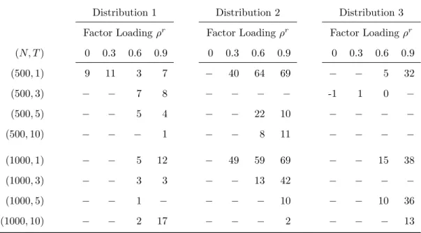
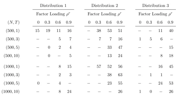
6.2.8 Monte Carlo Simulation Results: Efficiency
For Monte Carlo experiments, efficiency is measured by the root mean squared error (RMSE). Because Models L1 and L2 were generally the least accurate, I omit Models L1 and L2 from the following analysis. Tables 6.11 and 6.12 summarize both the MAD and efficiency gain comparisons betweenModel CandModel I. IfModel Cis more accurate (lower MAD) than Model I, the relative efficiency gain is reported for this specification. Otherwise, a hyphen appears in the cell. Consistent with the econometric theory, Model C does provide efficiency gains overModel Iwhen there is correlation between the error terms (ρr>0), and the efficiency generally improves as the correlation increases. The relative efficiency gain formula, in which β is the true coefficient value andβbs is the coefficient estimate from repetitions, is given by:
Relative Efficiency Gain = RMSE
M(I)−RMSEM(C)
RMSEM(I) , where RMSE = s
X
s
b
βs−β 2
. (6.9)
Table 6.11: Coefficient β1y Efficiency Gains for Model CRelative to Model I, by Specification
Distribution 1 Distribution 2 Distribution 3
Factor Loadingρr Factor Loadingρr Factor Loadingρr
(N, T) 0 0.3 0.6 0.9 0 0.3 0.6 0.9 0 0.3 0.6 0.9 (500,1) 9 11 3 7 − 40 64 69 − − 5 32
(500,3) − − 7 8 − − − − -1 1 0 −
(500,5) − − 5 4 − − 22 10 − − − −
(500,10) − − − 1 − − 8 11 − − − −
(1000,1) − − 5 12 − 49 59 69 − − 15 38 (1000,3) − − 3 3 − − 13 42 − − − − (1000,5) − − 1 − − − − 10 − − 10 36 (1000,10) − − 2 17 − − − 2 − − − 13
The relative RMSE is reported ifModel Cachieves a lower MAD thanModel I.
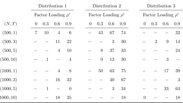
Table 6.12: Coefficient β2y Efficiency Gains for Model CRelative to Model I, by Specification
Distribution 1 Distribution 2 Distribution 3
Factor Loadingρr Factor Loadingρr Factor Loadingρr
(N, T) 0 0.3 0.6 0.9 0 0.3 0.6 0.9 0 0.3 0.6 0.9 (500,1) 7 10 4 6 − 43 67 74 − − − 32 (500,3) − − 11 22 − − 3 30 − 2 9 14 (500,5) − − 4 10 − 8 37 33 − − − 24 (500,10) − 1 − 4 − 0 13 30 − − 3 −
(1000,1) − − 4 8 − 50 63 75 − − 17 39 (1000,3) − − 16 32 − − 40 67 − − − 3 (1000,5) − 1 − 0 − − 3 34 − − 33 63 (1000,10) − − 18 35 − − − 18 0 − − 18
The relative RMSE is reported ifModel Cachieves a lower MAD than Model I.
Tables 6.13 and 6.14 show the RMSE comparison betweenModel CandModel E, in which the attitudinal responseris treated as an exogenous variable in the equation for outcomey. The results are similar to Tables 6.11 and 6.12; as the correlation between error terms strengthens, the efficiency gains for Model CoverModel Eincreases.