THE EFFICIENCY OF THE GAVER-STEHFEST METHOD TO SOLVE OF ONE-DIMENSIONAL GAS FLOW MODEL

Research Journal

Volume 11, Iss. 1, March 2017, pages 246–252

DOI: 10.12913/22998624/68138 Research Article

THE EFFICIENCY OF THE GAVER-STEHFEST METHOD

TO SOLVE ONE-DIMENSIONAL GAS FLOW MODEL

Małgorzata Wójcik1_{, Mirosław Szukiewicz}1_{, Paweł Kowalik}2_{, Wiesław Próchniak}2

1 _{Department of Chemical and Process Engineering,The Faculty of Chemistry, Rzeszow University of Technology,}

al. Powstańców Warszawy 12, 35-959 Rzeszow, Poland, e-mail: [email protected], [email protected]

2 _{Institute of New Chemical Synthesis, al. Tysiąclecia Państwa Polskiego 13a, 24-110 Pulawy, Poland, e-mail:}

[email protected], wiesł[email protected]

ABSTRACT

In this paper we examined the efficiency of one of the methods for numerical inver

-sion of the Laplace transform: the Gaver-Stehfest method to find a solution to a

one-dimensional gas flow model with axial dispersion. The algorithm was used to deter

-mine values of the axial dispersion coefficients D_L and Pèclet numbers Pe on the basis

of the pulse tracer technique. The obtained results of Pèclet numbers indicate that the gas flow is neither plug flow nor perfect mixing under operation condition. Numerical results are provided to confirm the efficiency of the presented method. Calculations were performed with the use of the CAS program type (Maple®).

Keywords: Laplace transform, method for numerical inversion of the Laplace trans

-form, axial dispersion coefficient, program Maple®_.

INTRODUCTION

Methods for numerical inversion of the La-place transform have enjoyed popularity in the field of science and engineering since at least the 1930s. The methods are a very helpful ‘tool of mathematics’ to solve problems of mathematics, physics, chemistry and engineering which are de-scribed inter alia by a system of differential equa-tions. In many cases, an analytical inversion of problems to the time domain can be difficult or even impossible to obtain. Many scientists used numerical algorithms of inverse Laplace trans-form to find a solution in the time domain of transport problems. For example, Chen [2] and Zhan et al. [13, 14] have successfully employed the Stehfest algorithm to obtain a solution in the time domain for the solute transport problems. Chen et al. [3] used the Crump method to obtain a solution of the radial dispersion in the real-time domain from the Laplace domain. Kocabas [8] presented two algorithms of inverse Laplace transform, the Stehfest method and the Dubner

and Abate method to modeling of tracer transport in heterogeneous porous media and estimating parameters of systems (e.g Pèclet number). Wang and Zhan [11] recommended the Stehfest meth-od, the Honig and Hirdes methmeth-od, and the Zakian method for dispersion problems. According to lit-erature reports, the method based on combination of Gaver functionals (the Gaver-Stehfest method) have been applied successfully to find solution in the time domain of transport problems [7, 9].

In this paper, the efficiency of method for nu-merical inversion of the Laplace transform based on combination of Gaver functionals – the Gaver-Ste-hfest method for solving an axial dispersion model is presented. Axial dispersion coefficients D_L and Pè-clet numbers Pe for measuring system are estimated.

The Gaver-Stehfest method

The Gaver-Stehfest method is a simple algo-rithm for the numerical inversion of the Laplace transform which has been used successfully by several authors for many problems [4, 10, 5].

This method approximates the time domain solution as [15]

(1) where V_k is described by the following equation

(1a)

The parameter N is called the Stehfest num-ber N. It is the numnum-ber of terms used in Eq. (1). Parameter N must be an even integer, it should be chosen by trial and error method. The preci-sion of calculation depends on the parameter N because the inversion is based on a summa-tion of N weighted values. Theoretically, the large value of parameter N determines a more accurate solution but if N is too large, the re-sults may be worsened due to round-off errors. Thus, a suitable choice of value N is impor-tant to achieve the most accurate solution [6]. Many authors propose a different value of the parameter N to obtain the most accurate solu-tion. For example, Cheng and Sidauruk recom-mended that optimal choice of N should be in a range from 6 to 20 [1].

DESCRIPTION OF THE EXPERIMENTS

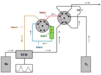
The main objective of this work is to find a sim-ple and effective method to find values of coefficients (D_L or Pe) of axial gas dispersion model. The scheme of the measuring system can be seen in Figure 1.

Zone 1: the pipe connected the 6-way valve outlet and the 6-way valve inlet; the length of the

zone: 2.0000•10-2 _{[m], the diameter of the zone:}

1.5875•10-3 _[m].

Zone 2: empty reactor; the length of the

zone: 1.7700•10-1 _{[m], the diameter of the zone:}

7.6500•10-3 _[m].

Zone 3: the pipe connected a reactor out-let and the 6-way valve; the length of the zone:

2.3500•10-1 _{[m], the diameter of the zone:}

Zone 4: the pipe connected the 6-way valve and TCD detector; the length of the zone: 5.5000•10-1

[m], the diameter of the zone: 1.5875•10-3 _[m]

The study was conducted as follows. The system was flushed for 15-30 minutes with a constant flow of heliumuntil a stable TCD signal was received. At the same time, the volume of sample loop (2.5000·10-7_{; 5.0000·10}-7 _[m3_{]) was flushed also with a constant flow of nitrogen. Next, the 6-way}

valves were opened to allow the flow of helium with the constant volumetric flow rate (of 3.3333·10-7 _or

5.0000·10-7_{or 6.6667·10}-7 _[m3_{/s]) through the sample loop, all zones to detector TCD. TCD signal was}

recorded. All experiments were conducted at pressure 1.0000·105 _{[Pa] and temperature 313 [K].}

ASSUMPTIONS OF THE MODEL

The presented model is based on the following assumptions:

• the system is operated under isothermal conditions and constant pressure,

• gases satisfy the equation of the state of an ideal gas.

MASS BALANCE OF THE PROCESS

Mass balance of the nitrogen in each zones can be described by the following a system of partial differential equations and the initial and boundary conditions:

Zone 1:

(2)

Zone 2:

(3)

Zone 3:

Zone 4:

(5)

c(L₁+L₂+L₃+L₄, t) corresponds concentration recorded by TCD-detector. We assumed that D_L,1 = D_L,3 =

D_L,4 due tu the same diameter of pipes. Inlet concentration can be described by rectangular pulse:

(5a)

where: C_T = P/R_g•T•103_{= 3.906·10}-2 _[kmol/m3_],

F_v– the volumetric flow rate [m3_/s].

RESULTS

To obtain the outlet concentration of tracer c(L₁+L₂+L₃+L₄, t), we solved a system of partial differen-tial equations Eq. (2-5) with appropriate inidifferen-tial and boundary conditions, by applying Laplace transform technique. The solution of model in Laplace domain may be written as

(6)

where:

(6a)

(6b)

where:

(6d)

s – the Laplace transform parameter.

Solution of Eq. (6) in the time domain was obtained using the Gaver-Stehfest method. The Gaver-Stehfest algorithm was chosen on the basis of previous tests. Accuracy of this algo-rithm was investigated for test functions and simplified model of a real gas flow. Details are presented in [12]. Parameter N called ‘parame-ter of accuracy’ for this method was de‘parame-termined by trial and error method. N = 30 was assumed as an optimal value for computations. All cal-culations were carried out with precision up to

48 decimal digits using Maple®_{17. Number of}

measurement points is equal to 70.

The obtained results are presented in Fig-ures 2 and 3. In all cases, very good fit be-tween numerical and experiment curves is

observed. The results showed that the Gaver-Stehfest method can solve the gas flow prob-lem with high accuracy (the minimal standard

deviation is equal to 7.1765·10-4_{, obtained for}

parameter N=30) and fast (time of calculations t=58.4 [s] for N=30). Proper value parameter N was determined by trial and error method as in [12]. Finally, N=30 was an optimal value of parameter N for solution of axial gas disper-sion model.

In this work, we used a pulse tracer tech-nique to determine the axial dispersion coef-ficients of the gas phase and value of Pèclet numbers in the zones of system. The nitrogen was been used as a tracer. The inverse problem (see Eq. 6) was solved by

combina-Fig. 2. Numerical (solid red line) and experimental (blue points) profiles of gas concentration for the volumetric

Fig. 3. Numerical (solid red line) and experimental (blue points) gas concentration profiles for the volumetric

flow rate 3.3333·10-7 _[m3_{/s] and the volume of sample loop 5.0000·10}-7 _[m3_{]. Screenshot of program Maple}®

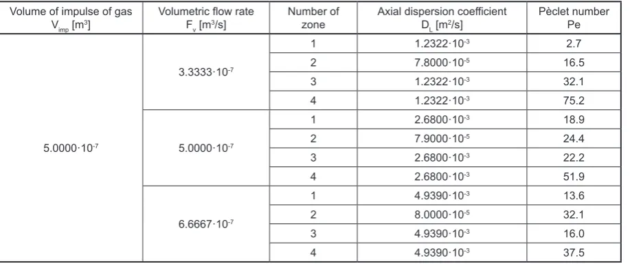
Table 1. Values of axial dispersion coefficients and Pèclet numbers

Volume of impulse of gas

V_imp [m3_] Volumetric flow rate_F v [m3/s]

Number of

zone Axial dispersion coefficientD_L [m2_/s] Pèclet number _Pe

2.5000·10-7

3.3333·10-7

1 7.7700·10-4 _4.3

2 7.8000·10-5 _16.5

3 7.7700·10-4 _51.0

4 7.7700·10-4 _119.3

5.0000·10-7

1 1.7826·10-3 _28.4

2 7.9000·10-5 _24.4

3 1.7826·10-3 _33.3

4 1.7826·10-3 _78.0

6.6667·10-7

1 3.1284·10-3 _21.5

2 8.0000·10-5 _32.1

3 3.1284·10-3 _25.3

4 3.1284·10-3 _59.2

tion of ‘trial –and-error’ procedure and inner optimization procedure of the program Maple.

As the correct value of parameter D_L was

ac-cepted this, for which the standard deviation

CONCLUSIONS

Table 2. Values of axial dispersion coefficients and Pèclet numbers

Volume of impulse of gas

V_imp [m3_] Volumetric flow rate_F v [m3/s]

Number of

zone Axial dispersion coefficientD_L [m2_/s] Pèclet number _Pe

5.0000·10-7

3.3333·10-7

1 1.2322·10-3 _2.7

2 7.8000·10-5 _16.5

3 1.2322·10-3 _32.1

4 1.2322·10-3 _75.2

5.0000·10-7

1 2.6800·10-3 _18.9

2 7.9000·10-5 _24.4

3 2.6800·10-3 _22.2

4 2.6800·10-3 _51.9

6.6667·10-7

1 4.9390·10-3 _13.6

2 8.0000·10-5 _32.1

3 4.9390·10-3 _16.0

4 4.9390·10-3 _37.5

2. The solution of the presented model fits ex-perimental results very well.

3. The gas flow is neither plug flow nor perfect mixing under operation condition.

4. The Computer Algebra System - Maple® al-lows the user to transform model equations to the Laplace domain, solve resulted set of equations and execute inverse Laplace trans-form just and without errors.

5. CAS – type programs are very helpful for re-searchers with unusual research or model.

REFERENCES

1. Cheng A.H-D, Sidauruk P. Approximate inversion

of the Laplace transform, The Mathematical Jour

-nal, 4, 1994, 76-82.

2. Chen C-S. Analytical and approximate solutions to radial dispersion from an injection well to a geological unit with simultaneous diffusion into adjacent strata, Water Resources Research, 21(8), 1985, 1069-1076.

3. Chen J-S., Liu C-W., Chen C-S., Yen H-D. A La

-place transform solution for tracer tests in a radial

-ly convergent flow field with upstream dispersion, Journal of Hydrology, 1996, 183(3-4), 263-275. 4. Chiang L-W. The application of numerical Laplace

inversion methods to groundwater flow and solute

transport problems, New Mexico Institute of Min

-ing and Technology, 1989.

5. Egonmwan A. O. The Numerical Inversion of the Laplace Transform: Gaver-Stehfest, Piessens, and

Regularized Collocation methods, LAP LAM

-BERT Academic Publishing, 2012.

6. Hassanzadeh H., Pooladi-Darvish M. Comparison of different numerical Laplace inversion methods

for engineering applications, Applied Mathematics and Computation, 189, 2007, 1966-1981.

7. Jaradat H. M., Jaradat M. M. M., AwawdehF., Mustafa Z., Alsayyed O. A new numerical method for heat equation subject to integral specifications, Journal of Nonlinear Science and Applications, 9, 2016, 2117-2125.

8. Kocabas I. Application of iterated Laplace trans

-formation to tracer transients in heterogeneous po

-rous media, Journal of the Franklin Institute, 348, 2011, 1339-1362.

9. Rezaei A., Zhan H., Zare M. Impact of thin aquita

-rds on two-dimensional solute transport in an aqui

-fer, Journal of Contaminant Hydrology, 152, 2013, 117-136.

10. Valkό P., Vajda S. Inversion of noise-free Laplace

transforms: towards a standardized set of test prob

-lems, Inverse Problems in Engineering, 10(5), 2002, 467-483.

11. Wang Q., Zhan H. On different numerical inverse Laplace methods for solute transport problems, Advances in Water Resources, 75, 2015, 80-92. 12. Wójcik M., Szukiewicz M., Kowalik P. Application

of numerical Laplace inversion methods in chemi

-cal engineering with Maple®. The Journal of Ap

-plied Computer Science Methods, 7(1), 2015, 5-15. 13. Zhan H., Wen Z., Gao G. An analytical solution

of two-dimensional reactive solute transport in

an aquifer-aquitard system, Water Resources Re

-search, 45(10), 2009.

14. Zhan H., Wen Z., Huang G., Sun D. Analytical solution of two-dimensional solute transport in an aquifer-aquitard system, Journal of Contaminant Hydrology, 2009, 107(3-4), 162-174.

15. Zhang J.Some innovative numerical approaches

for pricing American options, University of Wol