Research Journal
Volume 8, No. 24, Dec. 2014, pages 1–8
DOI: 10.12913/22998624/558 Research Article
Received: 2014.09.25 Accepted: 2014.10.25 Published: 2014.12.01
COMBINING FUZZY AND CELLULAR LEARNING AUTOMATA METHODS
FOR CLUSTERING WIRELESS SENSOR NETWORK TO INCREASE LIFE
OF THE NETWORK
Javad Aramideh1, Hamed Jelodar2
1 Department of Computer Engineering, Sari Branch, Islamic Azad University, Sari, Iran, e-mail: Aramideh. [email protected]
2 Department of Computer Engineering, Bushehr Branch, Islamic Azad University, Bushehr, Iran, e-mail: [email protected]
ABSTRACT
Wireless sensor networks have attracted attention of researchers considering their abundant applications. One of the important issues in this network is limitation of energy consumption which is directly related to life of the network. One of the main works which have been done recently to confront with this problem is clustering. In this paper, an attempt has been made to present clustering method which performs clustering in two stages. In the first stage, it specifies candidate nodes for being head cluster with fuzzy method and in the next stage, the node of the head cluster is deter-mined among the candidate nodes with cellular learning automata. Advantage of the clustering method is that clustering has been done based on three main parameters of the number of neighbors, energy level of nodes and distance between each node and sink node which results in selection of the best nodes as a candidate head of cluster nodes. Connectivity of network is also evaluated in the second part of head cluster determination. Therefore, more energy will be stored by determining suitable head clusters and creating balanced clusters in the network and consequently, life of the network increases.
Keywords: wireless sensor network, clustering, fuzzy logic, cellular learning automata.
INTRODUCTION
Wireless sensor networks which are used to collect information and study an environment multilaterally are composed of cheap sensors which have been dispersed in an environment and information collected with sensors should be transferred to a basic station. Since the sensor nodes have limited weight, size and cost which have direct effect on access to sources and con-sidering that nodes have batteries, processing ca-pability and limited communication and it is not proper to replace batteries in many applications, low power consumption is one of the essential needs in these networks and life of each sensor can be effectively increased by optimizing energy
consumption. In this paper, an attempt has been made to present a combined strategy for cluster-ing of dispersed sensors in the environment to lead to effective and efficient storage resulting in reduction of the consumed energy and increase the life of the network. In this paper, we present some performed works and the proposed method and results of simulation.
RELATED WORKS
Advances in Science and Technology Research Journal vol. 8 (23) 2014
2
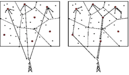
the network into some independent clusters, each with one head cluster which collects all the infor-mation from nodes inside its cluster. This head cluster sends information to the base center after data compression and Single-hop Communica-tion directly or in Multi-hop CommunicaCommunica-tion with lower number of hob and only with head cluster nodes. Clustering can reduce communication cost of most nodes considerably because they should only send information to the nearest head cluster instead of sending it directly to the base center which may be very far [Fahmy 2004].
Fig. 1. Single-hop Communication and Multi-hop Communication with clustering
SOME WORKS WHICH HAVE BEEN DONE
IN THE FIELD OF CLUSTERING
Xu et al. [2005] and Rosemark et al. [2005] have presented methods based on search. In these methods, a query has been created in a sink node and broadcasted in the network. Each node processes query by receiving it and sends it to its neighbors. After complete query was processed, the result will be returned to the sink node. In this scenario, some nodes process only queries and others broadcast them and obtain partial re-sults. They aggregate results and return them to sink node.
In some works by Bontempi et al. [2005], Virrankoski et al. [2005] and Soro et al. [2005],
network is first clustered and then head clusters
aggregate the data received from each cluster separately.
Lotfi Nejad et al., [2004] tried to study effect of relatively dependent data on efficiency of the
clustering methods in aggregation of data. They showed that dependence of data had a
consider-able effect on efficiency of clustering. It means that lower dependency of data lowers efficien -cy of clustering. They also showed that energy spent in a node is highly dependent on location
of that node in the network and the node which has longer distance from sink node consumes more energy and they also showed that life of the network had reverse relationship with energy consumption rate.
Other methods have been suggested for aggre-gation of data in the sensor network and Guestrin et al., tried to estimate data of a node in a time in-terval with a cubic function and send polynomial
coefficients to sink node instead of sending data
[Guestrin et al. 2004].
PROPOSED METHOD
As mentioned above, clustering is one of the considered methods for reduction of energy con-sumption in the wireless sensor networks. There-fore, in this paper, we decide to present a method for clustering of sensor network by combining two fuzzy method and cellular learning automata method to increase life of the network by reduc-ing energy of the network. The proposed method has composed of several sections which are men-tioned as follows.
Specifying candidate nodes for being head cluster
At the beginning of the proposed method, we will specify a candidate sensor nodes for being head cluster and for this purpose, we use fuzzy method. In this case, we use 3 factors effective on candidacy of a node for being head cluster in a network as input of fuzzy system. These factors include:
1) number of neighbor node (the nodes which are in communication range of each sensor), 2) remaining energy of sensor node, 3) distance between node and sink node.
Therefore, the used fuzzy system is composed of 3 inputs and 1 output and each of the inputs and also output of the system are divided into classes and we assign verbal words to each class and
ver-bal words are classified and assigned to each in -put and out-put.
Two inputs of the number of neighboring node and distance to sink node were divided into 3 classes with low, medium and high verbal words.
Only output of the fuzzy system which
speci-fies probability of candidacy of the sensor node
for becoming head cluster was also divided into
five very low, low, medium, high and very high
classes.
In the above fuzzy system for AND and OR,
Min and Max operators and Center of
grav-ity defuzzifier. General scheme of fuzzy system,
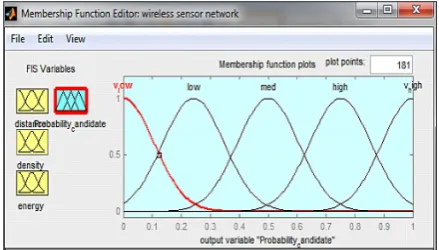
membership functions for input of energy level, output, fuzzy laws and a sample of test for de-termination of candidature of a sensor is shown and simulation of all of them has been done in the MATLAB software.
Fig. 2. General scheme of the presented fuzzy system
Fig. 3. Membership function relating to energy level
Fig. 4. Membership function relating to output
Set of the fuzzy laws applied in the discussed fuzzy system is as follows:
If (distance is low) and (density is low) and (en-ergy is low) then (Probability_candidate is v_low) If (distance is low) and (density is low) and (en-ergy is med) then (Probability_candidate is med)
Advances in Science and Technology Research Journal vol. 8 (23) 2014
4
If (distance is high) and (density is low) and (en-ergy is high) then (Probability_candidate is med) If (distance is high) and (density is low) and (ener-gy is v_high) then (Probability_candidate is high) If (distance is high) and (density is med) and (en-ergy is low) then (Probability_candidate is low) If (distance is high) and (density is med) and (en-ergy is med) then (Probability_candidate is med) If (distance is high) and (density is med) and (en-ergy is high) then (Probability_candidate is high) If (distance is high) and (density is med) and (energy is v_high) then (Probability_candidate is v_high) If (distance is high) and (density is high) and (en-ergy is low) then (Probability_candidate is low) If (distance is high) and (density is high) and (en-ergy is med) then (Probability_candidate is high) If (distance is high) and (density is high) and (ener-gy is high) then (Probability_candidate is v_high) If (distance is high) and (density is high) and (ener-gy is v_high) then (Probability_candidate is v_high)
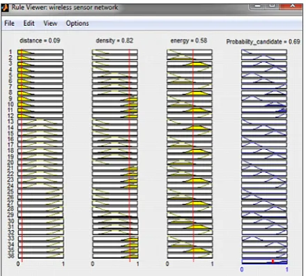
Fig. 5. A sample of a performed test for determination of candidate probability of a sensor\
It is necessary to note that the nodes are in-troduced as candidate node when the calculated probability in output of the fuzzy system is higher than the average rate.
Selection of head clusters among the candidate nodes
In this stage, we use cellular learning au-tomata for determination of the certain condition (becoming or not becoming head cluster) of the nodes which have introduced them as node of its
candidate head cluster in the previous stage. Since each node of the sensor has two conditions, then each one of the candidate nodes can select one of two states of cluster head and common node. For this work, we consider a learning automata cor-responding to each one of the candidate sensors and the corresponding automata can select one
of two states of CH and CN based on their prob -ability vector where CH indicates cluster head
and CN indicates common node and probability
of selecting each one of two actions is equal to 0.5. Probability of being cluster head based on different parameters decreases or increases based on different parameters with each selection. The parameters which we use for determination of cluster head among the candidate nodes include: • Energy rate. Since cluster head node should
collect information and send it to the sink node, it consumes more energy than other nodes. Therefore, attempt is made to select a node which has more energy than its neigh-bors. For this purpose, we use a difference between node energy and mean energy of its neighbors.
• Number of neighbor nodes. Since the en-ergy consumption rate in cluster head node is high, an attempt should be made to select the lowest number of cluster head among the can-didate nodes, therefore, the cancan-didate nodes which should be selected for becoming a clus-ter head when the number of its neighbors is higher than the mean number of its neighbor nodes, otherwise, the selected candidate node is found for becoming cluster head.
• Number of neighbor cluster head nodes. One of the important criteria for clustering is connectivity. It means that each node should be able to send its information to sink node. Therefore, either each node should have a clus-ter head node or one of its neighbors should be cluster head. Hence, in case a candidate node is selected as common node so no cluster head
node is its neighbor, it will be finally fined.
Another important point is that since the num-ber of cluster heads of the network should not be high, in case the candidate node which is selected as cluster head had neighbor cluster
head node should be fined.
receiv-5
Advances in Science and Technology Research Journal vol. 8 (23) 2014ing and sending data and information may be lost on the other hand. Therefore, consider-ing the capacity of the cluster, more balanced clusters will be created. Then, in case one of the candidate nodes is selected as common node and ratio of the number of its common neighbors to the number of its cluster head neighbors is higher than the capacity of
clus-ter, it will be fined and we consider the capac
-ity of cluster equal to 1.13N, based on some
performed works.
Considering the above-mentioned parameters, probability of performing that action will change by selecting each action with node automata. For rewarding and penalty, we use Relations (1) and
(2), where a is a reward coefficient and b is a pen
-alty coefficient.
pi(n + 1) = pi(n) + a[1 – pi(n)] (1) pi(n + 1) = 1 – pi(n + 1)
pi(n + 1) = (1 – b) pi(n) (2) pi(n + 1) = 1 – pi(n – 1)
In each round of node, reinforcement signal
iᵦ is calculated after selecting an action based on Relations (3) and (7). If iᵦ is equal to 1, the
selec-tive action is fined with Relation (2) and if it is
equal to 0, it will be rewarded in Relation (1). If
the selective action is head clustering, value of iᵦ
is obtained from Relation (3):
(2) In each round of node , reinforcement signal iᵦ is
calculated after selecting an action based on
Relations (3) and (7). If iᵦ is equal to 1, the selective action is fined with Relation ( 2) and if it is equal to 0, it will be rewarded in Relation (1). If the selective action is head clustering, value of iᵦ is obtained from Relation (3):
So that
e(n) is the remaining energy in the n-th round and eµ(n) is mean energy of node.
Ni is the number of neighbor node and Nµ is the mean number of neighbors in the neighbor nodes.
α j(n) is the selective action of node j.
Constant coefficient of we is the weight given parameters of energy in the clustering algorithm. Constant coefficient
of wu is the weight given to parameters relating to quality of clustering infrastructure and these two coefficients are
between 0 and 1 so that sum of coefficients becomes equal to 1:
If the selective action is selection of node as common node, value of iᵦ will be obtained from Relation (6):
So that:
(2) In each round of node , reinforcement signal iᵦ is
calculated after selecting an action based on
Relations (3) and (7). If iᵦ is equal to 1, the selective action is fined with Relation ( 2) and if it is equal to 0, it will be rewarded in Relation (1). If the selective action is head clustering, value of iᵦ is obtained from Relation (3):
So that
e(n) is the remaining energy in the n-th round and eµ(n) is mean energy of node.
Ni is the number of neighbor node and Nµ is the mean number of neighbors in the neighbor nodes.
α j(n) is the selective action of node j.
Constant coefficient of we is the weight given parameters of energy in the clustering algorithm. Constant coefficient
of wu is the weight given to parameters relating to quality of clustering infrastructure and these two coefficients are
between 0 and 1 so that sum of coefficients becomes equal to 1:
If the selective action is selection of node as common node, value of iᵦ will be obtained from Relation (6):
So that
where: e(n) is the remaining energy in the n-th round and eµ(n) is mean energy of node.
(2) In each round of node , reinforcement signal iᵦ is
calculated after selecting an action based on
Relations (3) and (7). If iᵦ is equal to 1, the selective action is fined with Relation ( 2) and if it is equal to 0, it will be rewarded in Relation (1). If the selective action is head clustering, value of iᵦ is obtained from Relation (3):
So that
e(n) is the remaining energy in the n-th round and eµ(n) is mean energy of node.
Ni is the number of neighbor node and Nµ is the mean number of neighbors in the neighbor nodes.
α j(n) is the selective action of node j.
Constant coefficient of we is the weight given parameters of energy in the clustering algorithm. Constant coefficient
of wu is the weight given to parameters relating to quality of clustering infrastructure and these two coefficients are
between 0 and 1 so that sum of coefficients becomes equal to 1:
If the selective action is selection of node as common node, value of iᵦ will be obtained from Relation (6):
So that
(4)
where: Ni is the number of neighbor node and Nµ is the mean number of neighbors in the neighbor nodes.
(2) In each round of node , reinforcement signal iᵦ is
calculated after selecting an action based on
Relations (3) and (7). If iᵦ is equal to 1, the selective action is fined with Relation ( 2) and if it is equal to 0, it will be rewarded in
Relation (1). If the selective action is head clustering, value of iᵦ is obtained from Relation (3):
So that
e(n) is the remaining energy in the n-th round and eµ(n) is mean energy of node.
Ni is the number of neighbor node and Nµ is the mean number of neighbors in the neighbor nodes.
α j(n) is the selective action of node j.
Constant coefficient of we is the weight given parameters of energy in the clustering algorithm. Constant coefficient
of wu is the weight given to parameters relating to quality of clustering infrastructure and these two coefficients are
between 0 and 1 so that sum of coefficients becomes equal to 1:
If the selective action is selection of node as common node, value of iᵦ will be obtained from Relation (6):
So that
(5)
where: αj(n) is the selective action of node j.
Constant coefficient of weis the weight given parameters of energy in the clustering algorithm.
Constant coefficient of wuis the weight given to parameters relating to quality of clustering
infra-structure and these two coefficients are between 0 and 1 so that sum of coefficients becomes equal to
1. If the selective action is a selection of node as a common node, value of βi will be obtained from Relation (6):
(2) In each round of node , reinforcement signal iᵦ is
calculated after selecting an action based on
Relations (3) and (7). If iᵦ is equal to 1, the selective action is fined with Relation ( 2) and if it is equal to 0, it will be rewarded in
Relation (1). If the selective action is head clustering, value of iᵦ is obtained from Relation (3):
So that
e(n) is the remaining energy in the n-th round and eµ(n) is mean energy of node.
Ni is the number of neighbor node and Nµ is the mean number of neighbors in the neighbor nodes.
α j(n) is the selective action of node j.
Constant coefficient of we is the weight given parameters of energy in the clustering algorithm. Constant coefficient
of wu is the weight given to parameters relating to quality of clustering infrastructure and these two coefficients are
between 0 and 1 so that sum of coefficients becomes equal to 1:
If the selective action is selection of node as common node, value of iᵦ will be obtained from Relation (6):
So that So that:
This stage is performed in several rounds. In each round, each sensor node selects one of the conditions of becoming or not becoming cluster head based on its probability vector and broadcasts a message to all of its neighbors and the message which contains node selective action, remaining energy and the number of its neighbors. After the specified time which all nodes received message of their neighbors, each node is rewarded or fined based on its selective action based on Relations (1) and (2) and increases or decreases probability of becoming or not becoming cluster head . In the next round, nodes select new state based on new probability and repeat operations.
Each node of which probability of becoming head cluster reaches zero or one selects a state based on probability vector and reaches stable condition. This algorithm continues until a clear percent of candidate nodes (95% in the performed tests) reach
stable conditions. At this time, all nodes select their state and this stage ends. Status of the major part of the candidate nodes has been determined while status of few candidate nodes may not be determined. There are statuses where some nodes of which status has been determined as common node are not in neighborhood of any cluster head node. Here, we add some candidate nodes to the cluster head nodes due to coverage of such common nodes and they are selected as cluster head node based on
having abundant neighbors compared
with the adjacent nodes
3. Formation of Cluster
After specifying status of the candidate nodes and determining cluster heads in the previous stages, it is time to create clusters. In
this stage, the cluster head nodes broadcast a message based on their geographical position to the adjacent nodes and then
common nodes select the nearest node as cluster head among cluster head neighbors. To create cluster, each common node sends a packet to its cluster head and identifies members of the cluster by collecting these packets and form cluster and then broadcast them to all nodes of the cluster based on time schedule. Time for submission of packet is specified by each one of the members.
4. Data Transmission
In this stage, common nodes send their data to cluster head nodes alternatively and with specified time intervals and node of the cluster head aggregates packets and sends it as a single packet to the sink node after all nodes in a cluster have sent their data to cluster head. In this stage, each common node of which data was sent is activated based on time schedule and is inactivated after sending packet to the sink node. The cluster head node will not be active in all time periods and is activated only when it wants to receive data of member nodes.
5. Change of Cluster Head
It is evident that energy of cluster head nodes is consumed faster than other member nodes due to higher activity and the network is disrupted. Under such condition, we use change of cluster head node to prevent this problem such that the member nodes send some of their remaining energy to the cluster head node in each data submission period and after the cluster head node sent the aggregated packet to the sink node, the cluster head node would calculate mean energy of the member nodes and if this energy rate is higher than the threshold limit, the node which has more energy will become cluster head and in the new time period, each node which sends data to it responds with message of chang_clustering and introduces the new cluster head node (Saeedian , 2011).
6. Calculating Energy Consumption Rate
In this paper, to calculate energy consumption rate of the sensors, it has been assumed that all sensors will send K bit data in each round. To calculate energy consumption of each sensor in each round, Relation (4) which has been known as Hizelman’s Relation will be used and this Relation is mentioned as follows.
This stage is performed in several rounds. In each round, each sensor node selects one of the conditions of becoming or not becoming cluster head based on its probability vector and broadcasts a message to all of its neighbors and the message which contains node selective action, remaining energy and the number of its neighbors. After the
specified time which all nodes received message of their neighbors, each node is rewarded or fined
based on its selective action based on Relations (1) and (2) and increases or decreases probability of becoming or not becoming cluster head. In the next round, nodes select new state based on new probability and repeat operations.
Each node of which probability of becoming head cluster reaches zero or one selects a state based on probability vector and reaches stable condition. This algorithm continues until a clear percent of candidate nodes (95% in the performed tests) reach stable conditions. At this time, all nodes select their state and this stage ends. The
status of the major part of the candidate nodes has
been determined while status of few candidate nodes may not be determined. There are statuses where some nodes of which status has been deter-mined as a common node are not in neighborhood of any cluster head node. Here, we add some can-didate nodes to the cluster head nodes due to cov-erage of such common nodes and they are selected as cluster head node based on having abundant
neighbors, compared with the adjacent nodes.
Formation of cluster
After specifying the status of the candidate nodes and determining cluster heads in the pre-vious stages, it is time to create clusters. In this stage, the cluster head nodes broadcast a message (3)
(6)
Advances in Science and Technology Research Journal vol. 8 (23) 2014
6
based on their geographical position to the
ad-jacent nodes and then common nodes select the
nearest node as cluster head among cluster head neighbors. To create cluster, each common node
sends a packet to its cluster head and identifies
members of the cluster by collecting these packets and form cluster and then broadcasts them to all nodes of the cluster based on time schedule. Time
for submission of packet is specified by each one
of the members.
Data transmission
In this stage, common nodes send their data to cluster head nodes alternatively and with
speci-fied time intervals and node of the cluster head ag -gregates packets and sends it as a single packet to the sink node after all nodes in a cluster have sent their data to cluster head. In this stage, each common node of which data was sent is activated based on time schedule and is inactivated after sending the packet to the sink node. The cluster head node will not be active in all time periods and is activated only when it wants to receive data of the member nodes.
Change of cluster head
It is evident that energy of cluster head nodes is consumed faster than other member nodes due to higher activity and the network is disrupted. Under such condition, we use change of cluster head node to prevent this problem such that the member nodes send some of their remaining en-ergy to the cluster head node in each data submis-sion period and after the cluster head node sent the aggregated packet to the sink node, the clus-ter head node would calculate mean energy of the member nodes and if this energy rate is higher than the threshold limit, the node which has more en-ergy will become cluster head and in the new time period, each node which sends data to it responds with message of chang_clustering and introduces the new cluster head node [Saeedian at al. 2011].
Calculating energy consumption rate
In this paper, to calculate energy consumption rate of the sensors, it has been assumed that all sensors will send K bit data in each round. To cal-culate energy consumption of each sensor in each round, Relation (4) which was known as Hizel-man’s Relation will be used and this Relation is mentioned as follows:
TX = ؏elec·K + ؏amp·d2 · K (8) where: K – is the number of the transmitted bit in
each round which is sent from each sen-sor node. K value is constant for all sensor nodes.
d – is distance between common sensor node and cluster head node. For the clus-ter head node, there is a distance between cluster head node and sink node.
Parameters ؏ampand ؏elec are regarded as energy which internal circuit of each sensor consumes at time of data transmission and is equal to constant
values. ؏amp isequal to 100 Pj/bit·m2 which is equivalent to 100·10-12 j and ؏
elecis equal to value
of 50 nj/bit which is equivalent to value of 50·10-9 j. The point is that the cluster head nodes consume energy for receiving data and there are different methods to calculate energy of the cluster head at time of receiving data from member sensors. In the method which has been used in this paper, the cluster head node receives n-bit packets based on the number of member nodes and converts them into n-bit packet and sends them. The difference is that we consider the consumed energy for this conversion. This consumed energy is known as EDAand its value is considered as 5·10-9 which is added to the consumed energy value for submission of data to sink node [Al-Obaidy et al. 2008].
SIMULATION
In this paper, we evaluate the proposed meth-od with 2 different scenarios and compare the above method with Leach’s algorithm to show
ef-ficiency. In this research, attempt has been made
to continue evaluation until the network has real value. For this reason, the network continues working until the number of the live nodes in the network is such that they create acceptable cover in the environment [Heinzelman et al. 2000].
In this paper, MATLAB software which is a suitable environment for simulation has been used for simulation and the constant parameters used in simulation are mentioned as follows: • The sensor nodes are dispersed in the
envi-ronment randomly and each node has range of sensor Rs and sensor environment of each node is a circle with radius of Rs.
• All nodes have equal energy and power at the beginning.
• Identification number of all nodes was recog -nized for sink node.
• The initial energy of all nodes is first 0.1 joules.
• In the performed tests, the network continues its activity until it has effective cover in the environment and when a node dies, its energy
reaches below 0.05 joules.
• To determine effective cover of the entire plate as set of points that is we produce points 0·0 to L·L for a environment with dimensions of L·L. at the end of each round, we check data submission and some points are present in sensor range of the active nodes.
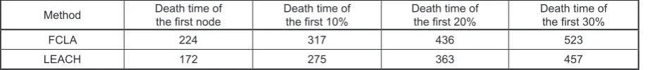
First scenario – studying death time of 10%, 20% and 30% of sensors. 100 sensors have been broadcasted in the environment with dimensions of 500·500 and sensor range of each sensor is equal to 20 and the diagram of number of live node relative to the number of executive round for the proposed method compared with LEACH algorithm (Figure 6, Table 1).
Second scenario – studying the number of effective executive round of the network. In this test, 30 sensors have been broadcasted in an environment with dimensions of 100·100 and the number of the executive round of the network has been compared with Leach algorithm until it cre-ates effective cover in the network (here, we con-sidered effective cover equal to cover above 59%).
Table 1. Comparing results of two algorithms in the first scenario
Method Death time of the first node Death time of the first 10% Death time of the first 20% Death time of the first 30%
FCLA 224 317 436 523
LEACH 172 275 363 457
Fig. 6. Diagram of the number of live node relative to the first scenario time
Advances in Science and Technology Research Journal vol. 8 (23) 2014
8
CONCLUSION
Clustering is one of the main works for re-duction of energy consumption and increase of life in the wireless sensor networks. For this reason, in this paper, attempt has been made to present a new method of clustering which is based on energy with combination of fuzzy and cellular learning automata (FCLA) and results of simulation prove that FCLA method shows clear preference over LEACH protocol in terms of increase of useful life of the network
(suspen-sion of the death time of the first node and initial
death percent of nodes) and also the number of executive rounds.
REFERENCES
1. Fahmy Y.S.: Distributed clustering in ad-hoc sen-sor networks: A hybrid, energy-efficient approach. In: Proceedings of IEEE INFOCOM, Vol. 1, 2004, 629–640.
2. Xu Y., Lee W.C., Xu J., Mitchell G.: Processing window queries in wireless sensor networks.IEEE International Conference on Data Engineeing, GA, April 2005.
3. Rosemark R., Lee W.C.: Decentralizing query pro-cessing in sensor networks. The Second Interna-tional Conference on Mobile and Ubiquitous Sys-tems. Netmarking and Service, CA, 2005, 270–280. 4. Bontempi G., Le Borgne Y.: An adaptive modular approach to the mining of sensor network data.
Pro-ceedings of the Workshop on Data Mining in Sensor Network, SLAM, SDM, CA, USA, April 2005. 5. Virrankoski R., Savvides A.: TASC: topology
adap-tive spatial clustering for sensor networks. In: IEEE International Conference on Mobile Adhoc and Sensor systems. DS, November, 2005.
6. Soro S., Heinzelman W.: Prolongingthe lifetime of wireless sensor networks via Uneven clustering. Proceedings of the 5th International Workshop on Algorithms for Wirelees, Mobile, April 2005. 7. Lotfi Nezhad M., Liang B.: Effect of partially
cor-related data on clustering in wireless sensor net-works. Proc. First IEEE Int’l Conf. Sensor and Ad Hoc Communications and Network, Santa Clara, California, October 2004.
8. Guestrin C., Bodik P., Thibaux R. , Paskin M., Mad-den S.: Distributed regression: an efficient frame-work for modeling sensor netframe-work data. Intel cor-poration, 2004.
9. Al-Obaidy M., Ayesh A., Sheta A.F.: Optimizing the communication distance of an ad hoc wireless sensor networks by genetic algorithms. Artif. Intell. Rev. 29, 2008, 183–194.
10. Heinzelman W.R., Chandrakasan A., Balakrishnan H.: Energy-efficient communication protocol for-wireless microsensor networks. IEEE, Proceedings of the 33rd Hawaii International Conference on System Sciences, 2000.