Volume 33 - Article 14 | Pages 391–424

(1)

DEMOGRAPHIC RESEARCH

A peer-reviewed, open-access journal of population sciences

DEMOGRAPHIC RESEARCH

VOLUME 33, ARTICLE 14, PAGES 391–424

PUBLISHED 1 SEPETEMBER 2015

http://www.demographic-research.org/Volumes/Vol33/14/ DOI: 10.4054/DemRes.2015.33.14

Research Article

Decomposing changes in life expectancy:

Compression versus shifting mortality

Marie-Pier Bergeron-Boucher

Marcus Ebeling

Vladimir Canudas-Romo

c

2015 Bergeron-Boucher, Ebeling & Canudas-Romo.

(2)

1 Background 392

2 Methods and data 394

2.1 Decomposing life expectancy 394

2.2 Decomposing senescent mortality: Gompertz 396 2.3 Extending the model beyond senescent mortality 398

2.3.1 Gompertz-Makeham 399

2.3.2 Siler 399

2.4 Data 401

3 Illustration 402

3.1 Gompertz decomposition 402

3.2 Gompertz-Makeham decomposition 404

3.3 Siler decomposition 405

3.4 Life expectancy and modal age at death 407

4 Discussion and conclusion 409

5 Acknowledgements 410

(3)

Decomposing changes in life expectancy:

Compression versus shifting mortality

Marie-Pier Bergeron-Boucher1

Marcus Ebeling2

Vladimir Canudas-Romo1

Abstract

BACKGROUND

In most developed countries, mortality reductions in the first half of the 20th century were highly associated with changes in lifespan disparities. In the second half of the 20th century, changes in mortality are best described by a shift in the mortality schedule, with lifespan variability remaining nearly constant. These successive mortality dynamics are known as compression and shifting mortality, respectively.

OBJECTIVE

To understand the effect of compression and shifting dynamics on mortality changes, we quantify the gains in life expectancy due to changes in lifespan variability and changes in the mortality schedule, respectively.

METHODS

We introduce a decomposition method using newly developed parametric expressions of the force of mortality that include the modal age at death as one of their parameters. Our approach allows us to differentiate between the two underlying processes in mortality and their dynamics.

RESULTS

An application of our methodology to the mortality of Swedish females shows that, since the mid-1960s, shifts in the mortality schedule were responsible for more than 70% of the increase in life expectancy.

CONCLUSIONS

The decomposition method allows differentiation between both underlying mortality pro-cesses and their respective impact on life expectancy, and also determines when and how one process has replaced the other.

1_{Max-Planck Odense Center on the Biodemography of Aging, University of Southern Denmark, Odense,}

Denmark.

2_{Max Planck Institute for Demographic Research, Rostock, Germany. University of Rostock, Institute of}

(4)

1. Background

Human mortality has undergone remarkable declines over the years. The increase in life expectancy is probably the best expression for the dramatic mortality decline in the last 170 years (Oeppen and Vaupel 2002). Improvements in living conditions, nutrition and medicine are among the main reasons for this development (Riley 2001; Oeppen and Vaupel 2002). These changes in economic, social, and sanitary conditions first triggered an important decline in infant, child, and early adult mortality, which contributed to the reduction in lifespan disparities (Wilmoth and Horiuchi 1999; Edwards and Tuljapurkar 2005; Vaupel, Zhang, and van Raalte 2011). As individuals became more homogeneous in their ages at death, a compression of the distribution of deaths in a more narrow age-interval was observed in many low-mortality countries in the first half of the twentieth century (Fries 1980; Wilmoth and Horiuchi 1999; Kannisto 2000, 2001; Cheung et al. 2009). Fries (1980) hypothesized that this dynamic can be interpreted as a compression of deaths against the upper limit of the human lifespan. Assuming a nearly negligible role for premature mortality, he stated the limit of the average age at death as approxi-mately 85 years, with 95% of all deaths occurring in an age range of 4 years deviation (Fries 1980). The “compression of mortality hypothesis” motivated a rich discussion on the occurrence and interpretation of this development. Several studies provided evidence for a compression, but emphasized that the achieved mortality levels differ substantially from Fries’ predictions (Nusselder and Mackenbach 1996; Wilmoth and Horiuchi 1999; Cheung et al. 2005).

After the period of strong compression, low-mortality countries entered a new era of change. Since the second half of the twentieth century, the main contributions to the increase in average age at death shifted from infant and early adult ages to old and very old-ages (Christensen et al. 2009). This generated changes in the mechanisms behind the increase in life expectancy (Wilmoth and Horiuchi 1999; Edwards and Tuljapurkar 2005; Smits and Monden 2009). The new mechanism behind improvement in life ex-pectancy is best illustrated by a shift in the distribution of death toward older ages with a shape remaining nearly constant (Yashin et al. 2001; Bongaarts 2005; Cheung et al. 2005; Cheung and Robine 2007; Canudas-Romo 2008). Vaupel (1986), Vaupel and Gowan (1986) and Bongaarts (2005) were among the first to articulate the idea of shifting mor-tality. Canudas-Romo (2008) deepens this idea by studying the variability around and the change of the modal age at death. He finds that over time mortality shifts to higher ages, with approximately constant variability in age at death. He concludes that the shifting mortality pattern might be the new dynamic behind mortality improvements, subsequent to the compression process.

(5)

Wilmoth and Horiuchi 1999; Kannisto 2000; Cheung et al. 2005). On the other hand, shifting mortality requires changes at old and very old-ages (Canudas-Romo 2008). Vau-pel, Zhang, and van Raalte (2011) report relatively stable variability patterns for survivors beyond age 50 in the last 100 years. Engelman, Caswell, and Agree (2014) and Engelman, Canudas-Romo, and Agree (2010), however, provide evidence for a modest expansion of lifespan variability for survivors at older ages, resulting from mortality improvement at these same ages.

The measurement of compression and shifting mortality is an important issue, as both dynamics translate differently into survival, mortality density and hazard distributions (Wilmoth and Horiuchi 1999). Alterations are, however, visible in all three functions due to their interrelation. For instance, in a mortality compression context, the survival curve becomes more rectangular with increasing concentration of deaths at old-age, which is a well-known phenomenon called rectangularization (Nusselder and Mackenbach 1996; Wilmoth and Horiuchi 1999; Cheung et al. 2005). Simultaneously, the old-age bulk of deaths in the distribution of death becomes more pronounced, thereby reducing variability of the age at death. In the hazard distribution, the slope becomes steeper, with mortality reductions being more pronounced at younger ages (Wilmoth and Horiuchi 1999; Robine 2001).

In a shifting mortality context, these three functions also undergo transformations. The downward slope of the survival curve will shift to higher ages with an equal shape. Similarly, the density distribution will shift towards older ages with a shape also remain-ing constant. In the hazard distribution, the same pattern requires a constant slope de-picted by a parallel shift of the logarithmic force of mortality toward higher ages (Bon-gaarts 2005; Canudas-Romo 2008). In this context, Bon(Bon-gaarts (2005) suggested fixing the shape parameter of mortality models and assumed that only scale and background pa-rameters can vary over time. Vaupel (2010) also describes a postponement of senescence rather than a fundamental change of the age-pattern of mortality for the period starting around 1950.

(6)

2001; Bongaarts 2005; Cheung and Robine 2007; Canudas-Romo 2008, 2010; Ouellette and Bourbeau 2011; Horiuchi et al. 2013).

Therefore, compression and shifting mortality are observed respectively by changes in the variability of the age at death and in the modal age at death. Both dynamics also have different implications regarding changes in mortality: the former reflects changes in lifespan disparities, while the latter provides information about changes in the timing of mortality.

Considering the two periods of change in mortality development, two questions arise. First, what is the impact of compression and shifting mortality dynamics on the increase of life expectancy over time? Second, how and to what extent did one process replace the other? Additionally, considering the impact of child and young adult mortality reduc-tions on the appearance of compression, one might further ask, if only adult and old-ages mortality is analyzed, how does the impact of both dimensions change?

To approach these questions, a new methodology to study changes in compression and shifting mortality over time and their effect on life expectancy is presented. We quantify the gains in life expectancy due to changes in the timing of mortality and changes in lifes-pan disparities, respectively. Using newly developed parametric expressions of the force of mortality (Horiuchi et al. 2013; Missov et al. 2015), we decompose the change in life expectancy between two distributions by the contribution of a shift in the modal age at death and a change in variability of the age at death.

This paper is divided into four sections, with this background as the first section. In the following section, we introduce the decomposition methodology, at first in general terms and then for the Gompertz, Gompertz-Makeham and Siler models. The third sec-tion presents an illustrasec-tion of the methodology applied to discrete data, followed by the fourth section, in which we present our conclusions.

2. Methods and data

2.1 Decomposing life expectancy

(7)

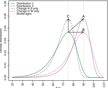
vari-ability and shifting effects using a recent expression of the Gompertz mortality model. Figure 1 shows the distribution of deaths for Gompertz parameters under two scenar-ios. It illustrates how changes in mortality can be decomposed into effects due to changes in variability and the shifting of mortality. Assuming a general change of mortality be-tween the two distributions (in Figure 1 as the arrow denoted as A), the shifting effect is the hypothetical change resulting only if the modal age at death (M) would have changed between those two distributions (in Figure 1 as arrow B). The variability effect is the hy-pothetical change produced only if the slope of the hazard function (β) changes from one distribution to another (in Figure 1 as arrow C). The latter transformation C, of changing the slope of the hazard distribution, also changes the shape of the density distribution, and thus their variability (Wilmoth 1997).

Changes in life expectancy at birth over time (denoted as e˙0,t) can thus be decom-posed into two components

˙

e0,t= ∆β + ∆M, (1)

where∆βand∆M are the gains in life expectancy resulting from changes in the shape parameter and modal age at death, respectively. In the following section we present the methodology of the decomposition for the Gompertz force of mortality and then general-ize it to other parametric functions of mortality.

Figure 1: Illustration of the shifting and variability effects in the density

function of the distribution of deaths for simulated data from a Gompertz model with a combination of shape parameters

β1= 0.10andβ2= 0.13and modal ages at deathM1= 75and

M2= 90

0.00

0.01

0.02

0.03

0.04

0.05

0.06

Age

Density distr

ib

ution

20 30 40 50 60 70 80 90 ₁₀₀ ₁₁₀

Distribution 1 Distribution 2 Change in β only Change in M only Modal ages

A

(8)

2.2 Decomposing senescent mortality: Gompertz

Gavrilov and Gavrilova (1991) defined the Gompertz (1825) law of mortality as one of the most successful models expressing mathematically the senescent age-pattern of mor-tality. In this article, we refer to senescent mortality as the increase over age in the force of mortality occuring after a certain age, representing aging and physiological deteriora-tion (Bongaarts and Feeney 2002; Bongaarts 2005; Horiuchi et al. 2013). The Gompertz approach allows a good approximation of adult mortality patterns over age and time for many countries. However, the Gompertz model does not fit infant, child and oldest-old mortality well. Other parametric models, such as the Makeham (1860) and Siler (1979), have addressed some of these problems by including additional parameters capturing background and infant mortality. The Gompertz model is, however, broadly used to de-scribe the distribution of adult death from age 30 to 90, having the advantage of being simple and offering a good fit to senescent mortality. The decomposition methodology in-troduced here will be presented through the Gompertz model, but it will be demonstrated that the method can be applied to other parametric models.

It has been shown by Horiuchi et al. (2013) and Missov et al. (2015) that the hazard rate as expressed by the Gompertz model can be rewritten using the modal age at death instead of the timing parameterαtas

µx,t=αteβtx=βteβt(x−Mt), (2)

whereβtis the shape parameter at timetof the Gompertz hazard functionµx,t, andMt is the modal age at death. This parametrization has some advantages: 1) the parameter

Mt has a clearer interpretation thanαt(Horiuchi et al. 2013), and 2) there is a lower correlation between the parameters when the Gompertz is expressed using the modal age at death (Missov et al. 2015).

The parametrization presented in equation (2) also gives a starting point for decom-posing changes in life expectancy due to changes in variability and shifting mortality. Shifting mortality is observed through changes in the modal age at death, which is cap-tured by the parameterMt. Additionally, as presented in Appendix A, it can analytically be shown that the shape parameterβtis the main carrier of variability changes.

Let a dot on top of a variable denote its derivative with respect to time (Vaupel and Canudas-Romo 2003). The change over time in the force of mortality (µ˙x,t) can be de-composed into respective components of change for the shape (β˙t) and the mode (M˙t):

˙

µx,t= ˙βt

µx,t( 1

βt

+x−Mt)

−M˙t [βtµx,t]. (3)

(9)

multiplied by a weighting function of the corresponding hazard rate, denoted asfi(µx,t), withicorresponding to the parametersβandM,

˙

µx,t= ˙βtfβ(µx,t) −M˙tfM(µx,t). (4)

As with the hazard distribution, we can derive the time change of life expectancy. In general terms, life expectancy at birth is expressed as

e0,t=

Z ω

0

la,tda,

wherela,t is the survival function and the radix of the population is one. Therefore, changes in life expectancy at birth through time (e˙0,t) can be expressed by:

˙

e0,t=

Z ω

0 ˙

la,tda=−

Z ω

0

la,t

Z a

0 ˙

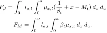
µx,tdxda, (5)

wherel˙a,tis the time derivative of the survival functionla,t. By substituting equation (4) in equation (5), we can estimate the change in life expectancy at birth due to changes in the modal age at death and changes in the shape parameter as:

˙

e0,t=−β˙t

Z ω

0

la,t

Z a

0

fβ(µx,t)dxda

| {z }

∆β

+ ˙Mt

Z ω

0

la,t

Z a

0

fM(µx,t)dxda

| {z }

∆M

. (6)

The first term in equation (6) represents the gain in life expectancy resulting from a change in variability (∆β), corresponding to a compression pattern, while the second term is the gain in life expectancy produced by a shift in the modal age at death (∆M), indicating a shifting pattern. These are the equivalent terms of equation (1) in the Gom-pertz model.

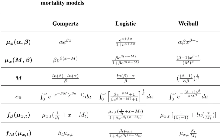
Equations (4) and (6) allow further generalizations to other parametric models ex-pressing senescent mortality using the modal age at death (M) and a shape parameter (β). Horiuchi et al. (2013) present this parametrization for the Logistic and Weibull mod-els. Table 1 includes the elements of the decomposition equations for the Gompertz, Logistic and Weibull models.

(10)

Table 1: Hazard (µx), modal age at death (M), life expectancy at birth (e0)

and decomposition weights (fβ(µx,t)andfM(µx,t)) for three

mortality models

Gompertz Logistic Weibull

µx(α,β) αeβx e

α+βx

1+eα+βx αβx

β−1

µx(M,β) βeβ(x−M) βeβ(x−M)

1+βeβ(x−M)

(β−1)xβ−1 (M)β

M ln(β)−_βln(α) ln(β_β)−α ((β_αβ−1))β1

e0 R

ω 0 e

−e−βM(eβa−1)_da Rω

0

h _βe−βM₊₁

βeβ(a−M)₊₁

iβ1

da Rω

0 e

−(β−1)aβ

βM β _da

fβ(µx,t) µx,t(_β1_t +x−Mt)

µx,t(_βt1+x−Mt)

1+βteβt(x−Mt) µx,t[ 1

(βt−1)+ln(

x

Mt)]

fM(µx,t) βtµx,t

βtµx,t

1+βteβt(x−Mt) µx,t

βt

Mt

Note: To simplify the equations, the time component (t) was not added as subscript to the parametersαt,βtand

Mtin the first four lines of the table. However, the parameters can also vary over time (t) in these equations.

2.3 Extending the model beyond senescent mortality

With the previous methodology, only senescent mortality can be decomposed. The de-composition is thus limited to adult and old-age mortality, and might bring only limited understanding of mortality changes over time. As mentioned previously, compression of mortality has been strongly linked to reductions in infant, child and early adult mortality, which is not considered when decomposing the Gompertz model. Modeling mortality at all ages needs more complex models, and additional parameters often need to be added.

Equation (1) can be generalized to allow the inclusion of parameters other thanβand

M, as

˙

e0,t= X

i=1

(11)

where∆iis the change in life expectancy at birth due to a change in the parameteri.

2.3.1 Gompertz-Makeham

A Makeham (1860) variant can be added to each of the models presented in Table 1 (Horiuchi et al. 2013). Assuming that the modal age at death (Mt) estimated by the Gompertz model in equation (2) applies to the Gompertz-Makeham model, the hazard function can be expressed as

µx,t=ct+βteβt(x−Mt), (8)

wherectis the Makeham term. Adding the parameterctimproves the fit of the Gompertz function at younger ages, but still without capturing the decrease in infant mortality. The Makeham term is an age-independent component which captures the extrinsic or “back-ground” mortality risk. The Makeham term has a more influential effect at younger ages and is often associated with adult or early adult mortality, which is especially important for the variability effect.

Equivalent to the decomposition presented in equation (6), we can estimate the change in adult life expectancy due to changes in the different parameters of the Gompertz-Makeham model using equation (5). As expressed by equation (7), change in life ex-pectancy is then estimated as

˙

e0,t=−c˙t

Z ω

0

la,ta da

| {z }

∆c

−β˙t

Z ω

0

la,t

Z a

0

[eβt(x−Mt)_{(1 +}_β

t(x−Mt))]dx da

| {z }

∆β

+ ˙Mt

Z ω

0

la,t

Z a

0

[β_t2eβt(x−Mt)_]_{dx da}

| {z }

∆M

, (9)

wherec˙tis the change in the background mortality level,β˙tis the change in the rate of mortality increase over age andM˙tis the change in the modal age at death.

2.3.2 Siler

(12)

µx,t=αte−btx+ct+βteβt(x−Mt), (10)

whereαtandctare timing parameters for infant and background mortality, the parame-tersbtandβtare the constant rates of mortality change over age for infant and senescent mortality, respectively, andMtis the modal age at death. By including the infant and background parameters, the Siler model provides a more detailed estimation of the vari-ability and shifting effect by modeling mortality at all ages.

Decomposition of changes in the Siler model is expressed by changes in 5 different parameters: α˙tis the change with respect to t in the initial level of mortality (age 0), ˙

btis the change in the rate of infant mortality decrease over age,c˙tis the change in the background mortality level,β˙tis the change in the rate of mortality increase over age for senescent mortality, andM˙tis the change in the modal age at death.

As generally presented in equation (7), the gain in life expectancy at birth for the Siler model is estimated by

˙

e0,t=−α˙t

Z ω

0

la,t

Z a

0

[e−btx_]_{dx da}

| {z }

∆α

+ ˙bt

Z ω

0

la,t

Z a

0

[αte−btxx]dx da

| {z }

∆b

−c˙t

Z ω

0

la,ta da

| {z }

∆c

−β˙t

Z ω

0

la,t

Z a

0

[eβt(x−Mt)_{(1 +}_β

t(x−Mt))]dx da

| {z }

∆β

+ ˙Mt

Z ω

0

la,t

Z a

0

[β_t2eβt(x−Mt)_]_{dx da}

| {z }

∆M

. (11)

(13)

will refer to the senescent modal age at death as the modal age at death.

When using the Gompertz model, the variability effect is captured by the parameterβt (Appendix A) and the shifting effect by the parameterMt. However, with a Gompertz-Makeham model or a Siler model, more parameters will influence variability changes. Canudas-Romo (2010) analytically demonstrated that, in a mortality declining scenario, as the one experienced in developed countries, the mode will be maintained when re-duction of mortality occurs at younger ages than the modal age at death. Using a Siler model, Engelman, Caswell, and Agree (2014) showed that improvement in childhood components of mortality (αtandbt) and in background mortality parameter (ct) influ-enced lifespan variability reduction. The first four terms of the above equation would then have an impact on variability reduction. The variability effect could then be divided into four distinct effects:α˙t,b˙t,c˙tandβ˙t. The shifting effect is still captured byM˙t. This partition between the five Siler parameters emphasizes the impact of changing mortality at young ages on lifespan disparities, in contrast with the effect of mortality reductions at older ages on shifting mortality.

2.4 Data

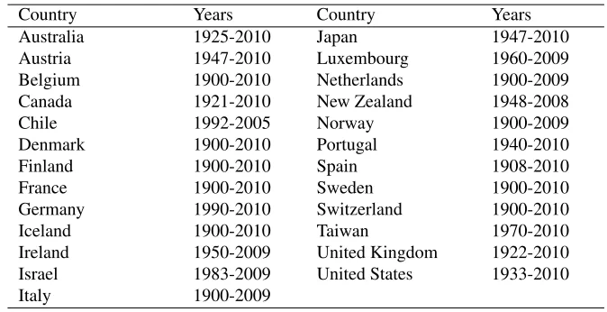
The data source used in this study is the Human Mortality Database (HMD: http://www. mortality.org). The HMD (2015) compiles census and vital statistics information for the populations of entire countries. The HMD has high quality historical mortality data for industrialized countries; the data series are constructed according to a common protocol, making the HMD a unique comparison tool. For our illustrations, data for all the HMD countries, excluding Eastern European countries, have been used for years 1900 to 2010 (Table 2). We justify the data exclusion because there are different age-patterns of mortal-ity in the excluded countries than to those included in the illustrations in recent decades. Nevertheless, our methodology can easily be extended to those countries although with different mortality parameters.

The decomposition is applied to the mortality of Swedish females and to the average female mortality in the selected HMD countries4. The Gompertz, Gompertz-Makeham and Siler models are fitted to observed mortality trends using a Poisson log-likelihood procedure. The estimation procedures of derivatives such as those in equations (6) to dis-crete data are presented in Appendix B.

4_{The parameters of the mortality models are estimated for each country independently and then averaged over}

(14)

Table 2: Selected HMD countries and years with available data used for the illustration

Country Years Country Years

Australia 1925-2010 Japan 1947-2010

Austria 1947-2010 Luxembourg 1960-2009

Belgium 1900-2010 Netherlands 1900-2009

Canada 1921-2010 New Zealand 1948-2008

Chile 1992-2005 Norway 1900-2009

Denmark 1900-2010 Portugal 1940-2010

Finland 1900-2010 Spain 1908-2010

France 1900-2010 Sweden 1900-2010

Germany 1990-2010 Switzerland 1900-2010

Iceland 1900-2010 Taiwan 1970-2010

Ireland 1950-2009 United Kingdom 1922-2010

Israel 1983-2009 United States 1933-2010

Italy 1900-2009

Source: HMD (2015)

3. Illustration

3.1 Gompertz decomposition

Table 3 presents the decomposition of life expectancy at age 30 byM andβfor Swedish females at the beginning, middle, and end of the 20th century and for the HMD females average, between 2000 and 2005. For the three periods selected and for both populations, changes in the modal age at death (∆M) are the main components driving the change in life expectancy.

(15)

Table 3: Female life expectancy at age 30 (e30,t) and its decomposition due to

changes in the Gompertz parameters, Sweden and HMD average, 1900, 1950, and 2000

Sweden HMD Average

1900 1950 2000 2000 (min, max)

e30,t 37.82 44.18 52.04 51.43 (49.23, 54.79) e30,t+5 38.21 45.56 52.72 52.45 (50.40, 55.67)

˙

e30,t 0.39 1.39 0.68 1.03

∆β -0.17 0.09 0.05 0.09 (-0.11, 0.22)

∆M 0.56 1.30 0.63 0.94 (0.48, 2.08)

∆β+ ∆M 0.39 1.39 0.68 1.03

Source:HMD (2015) and authors’ own calculation.

Note:By rounding the numbers to the second decimal point in the table, the sum of the contributions (P

∆i)

might differ slightly from the difference in life expectancy (˙e30,t).

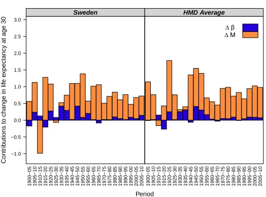
Figure 2: Trends over time of the Gompertz parameters’ contribution to

changes in female life expectancy at age 30 (e˙30,t), Sweden and

HMD average, 1900-2010

Period

Contr

ib

utions to change in lif

e e

xpectancy at age 30

−1.0 −0.5 0.0 0.5 1.0 1.5 2.0 2.5 3.0

1900−05 1905−10 1910−15 1915−20 1920−25 1925−30 1930−35 1935−40 1940−45 1945−50 1950−55 1955−60 1960−65 1965−70 1970−75 1975−80 1980−85 1985−90 1990−95 1995−00 2000−05 2005−10

Sweden

1900−05 1905−10 1910−15 1915−20 1920−25 1925−30 1930−35 1935−40 1940−45 1945−50 1950−55 1955−60 1960−65 1965−70 1970−75 1975−80 1980−85 1985−90 1990−95 1995−00 2000−05 2005−10

HMD Average

∆ β ∆ M

(16)

Changes in variability of senescent mortality alone would not have been sufficient to generate the important gains in life expectancy at age 30 observed since 1900. An ex-planation for this small variability effect compared with the important shifting effect for senescent mortality still needs to be provided. A possible explanation is that as only senescent mortality is analyzed by the Gompertz model, it does not consider the ages essentially responsible for mortality compression, i.e., infant, child and early adult (Che-ung and Robine 2007). To address the latter aspect of how mortality at yo(Che-ung ages has influenced changes in life expectancy, we present results for the Gompertz-Makeham and Siler models in the next sections.

3.2 Gompertz-Makeham decomposition

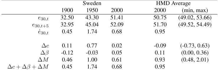
The Gompertz-Makeham model can help us understand the impact of early adult mor-tality changes on compression and shifting mormor-tality. Table 4 presents an application of the decomposition of life expectancy at age 30 using the Gompertz-Makeham model for Swedish and HMD average females at three points in time. Among the parameters influ-encing variability changes (βandc), the Makeham term (c) has a similar influence on life expectancy changes than the shape parameterβ, for most of the times studied in Table 4.

changes in the Gompertz-Makeham parameters, Sweden and HMD average, 1900, 1950, and 2000

Sweden HMD Average

1900 1950 2000 2000 (min, max)

e30,t 32.50 43.30 51.41 50.75 (49.02, 53.66) e30,t+5 32.95 45.04 52.09 51.70 (49.52, 54.49)

˙

e30,t 0.45 1.74 0.68 0.95

∆c 0.11 0.77 0.02 -0.09 (-0.73, 0.63)

∆β -0.12 -0.03 0.05 0.11 (0.00, 0.36)

∆M 0.46 1.00 0.61 0.93 (0.48, 2.01)

∆c+ ∆β+ ∆M 0.45 1.74 0.68 0.95

Note: By rounding the numbers to the second decimal point in the table, the sum of the contributions (P

∆i)

might differ slightly from the difference in life expectancy (˙e30,t).

(17)

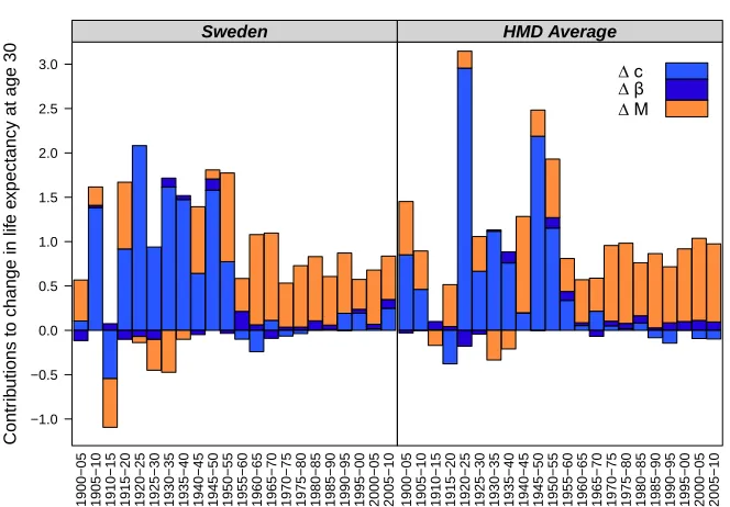
by changes in the parameterc. After this initial period of variability decline, changes in life expectancy at age 30 are mainly the result of shifting mortality (∆M).

The inclusion of a parameter capturing early adult background mortality appears es-sential, then, to demonstrate the effect of variability reduction on life expectancy at age 30. Figure 8 in Appendix C shows similar results for the selected HMD countries. The next section presents an application of the Siler decomposition, in order to understand the role of infant mortality on the changes in life expectancy.

Figure 3: Trends over time of the Gompertz-Makeham parameters’

contribution to changes in female life expectancy at age 30 (e˙30,t),

Sweden and HMD average, 1900-2010

Period

Contr

ib

e e

xpectancy at age 30

−1.0 −0.5 0.0 0.5 1.0 1.5 2.0 2.5 3.0

1900−05 1905−10 1910−15 1915−20 1920−25 1925−30 1930−35 1935−40 1940−45 1945−50 1950−55 1955−60 1960−65 1965−70 1970−75 1975−80 1980−85 1985−90 1990−95 1995−00 2000−05 2005−10 Sweden

1900−05 1905−10 1910−15 1915−20 1920−25 1925−30 1930−35 1935−40 1940−45 1945−50 1950−55 1955−60 1960−65 1965−70 1970−75 1975−80 1980−85 1985−90 1990−95 1995−00 2000−05 2005−10 HMD Average

∆ c ∆ β ∆ M

3.3 Siler decomposition

(18)

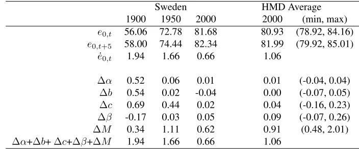
to the Gompertz-Makeham decomposition, the results suggest that changes in life ex-pectancy at birth before the 1950s were mainly the result of variability reductions. Gains in life expectancy due to changes in the parameterβare still small, and the main gains are due to variability reductions coming from changes in infant and background parameters.

Since the mid-1960s, the modal age at death has been the key parameter leading the changes in life expectancy. Changes in the modal age at death were responsible for more than 70% of the increase ine0,t since 1965 for females from both Swedish and HMD average. Figure 9 in Appendix C presents similar results for 25 of the HMD countries.

changes in the Siler parameters, Sweden and HMD average, 1900, 1950 and 2000

Sweden HMD Average

1900 1950 2000 2000 (min, max)

e0,t 56.06 72.78 81.68 80.93 (78.92, 84.16) e0,t+5 58.00 74.44 82.34 81.99 (79.92, 85.01)

˙

e0,t 1.94 1.66 0.66 1.06

∆α 0.52 0.06 0.01 0.01 (-0.04, 0.04) ∆b 0.54 0.02 -0.04 0.00 (-0.07, 0.05) ∆c 0.69 0.44 0.02 0.04 (-0.16, 0.23) ∆β -0.17 0.03 0.05 0.09 (-0.07, 0.26)

∆M 0.34 1.11 0.62 0.91 (0.48, 2.01)

∆α+∆b+∆c+∆β+∆M 1.94 1.66 0.66 1.06

∆i)

(19)

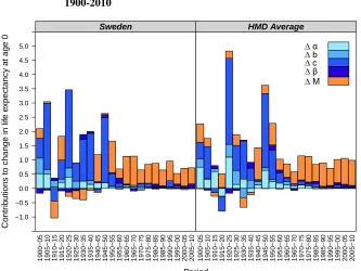
Figure 4: Trends over time of the Siler parameters’ contribution to changes in female life expectancy at age 0 (e˙0,t), Sweden and HMD average,

1900-2010

Period

Contr

ib

e e

xpectancy at age 0

−1.0 −0.5 0.0 0.5 1.0 1.5 2.0 2.5 3.0 3.5 4.0 4.5 5.0

1900−05 1905−10 1910−15 1915−20 1920−25 1925−30 1930−35 1935−40 1940−45 1945−50 1950−55 1955−60 1960−65 1965−70 1970−75 1975−80 1980−85 1985−90 1990−95 1995−00 2000−05 2005−10 Sweden

1900−05 1905−10 1910−15 1915−20 1920−25 1925−30 1930−35 1935−40 1940−45 1945−50 1950−55 1955−60 1960−65 1965−70 1970−75 1975−80 1980−85 1985−90 1990−95 1995−00 2000−05 2005−10 HMD Average

∆ α ∆ b ∆ c ∆ β ∆ M

Note:Appendix D presents these results in terms of relative differences.

3.4 Life expectancy and modal age at death

(20)

Figure 5: Modal age at death and life expectancy at birth and their respective segmented regression for females, Sweden and HMD average, 1900-2010

Year

Lif

e e

xpectancy at age 0 / Modal age at death

50 55 60 65 70 75 80 85 90

1900 1920 1940 1960 1980 2000 0.314

−0.021

0.151 0.134

Sweden

1900 1920 1940 1960 1980 2000 0.343

0.040 _0.184

0.138

HMD Average

Life expectancy at birth Modal age at death Segmented regression

Note: The slopes and breakpoints of the modal age at death and life expectancy trends are calculated

with a segmented regression methodology (Camarda, Vallin, and Mesl´e 2012).

A second period followed in which the mode begins to increase at a faster pace while life expectancy increase keeps its previous pace. Between 1940 and 1965, the mode contribu-tion to changes in life expectancy increased, while variability contribucontribu-tions gradually lost importance. During these years, variability contributions to changes in life expectancy decreased from more than 60% to less than 30% of the total gains (Appendix D). This period is one of acceleration in the increase of the modal age at death and marks the transition from compression to shifting mortality.

(21)

4. Discussion and conclusion

Using recent parametrization of the Gompertz model, we separated changes in life ex-pectancy by the variability reduction effect, captured byβ, from the shifting mortality effect, captured byM. The methodology is then extended to other parametric repre-sentations of mortality, and particularly to the Gompertz-Makeham and Siler models, to consider the effect of young adult, child and infant mortality changes. This new de-composition method, using parametric models, allows us to understand and quantify the respective impact of shifting mortality and variability changes on life expectancy.

Our results suggest that mortality compression was the main driver of change in life expectancy at birth before the 1950s, due to a decrease in infant and background mor-tality. After this period, changes in life expectancy became gradually dependent on the shift in the senescent modal age at death. These results are consistent with the findings of other studies looking at changes in the modal age at death and at different variability measures (Wilmoth and Horiuchi 1999; Robine 2001; Yashin et al. 2001; Canudas-Romo 2008). The results also confirm the increasing importance of the modal age at death as a key indicator of lifespan. The modal age at death has increased since the beginning of the 1940s and has become the main driver of longevity extension since the 1960s. An impor-tant feature of this indicator is that, in populations that experience declining mortality, its change is only determined by old-age mortality.

In the above illustrations, the results of the decomposition are presented for female life expectancy only. However, similar results are found when decomposing male life expectancy, but with a shifting pattern appearing later in time. Shifting mortality became the main driver of life expectancy increase in the late 1970s for males (results available from the authors).

We asked previously how and to what extent, one process replaced the other. Our methodology allows us to observe and quantify the gradual replacement of a compres-sion pattern by a shifting pattern in a relatively short period of time. We can also observe that, even if shifting the modal age at death is explaining a great deal of the life expectancy increase nowadays, lifespan variability reductions still play a role in mortality changes.

(22)

The choice of the parametric model for senescent mortality might also have influ-enced the results. The illustration section presented the application of the methodology to discrete data using a Gompertz model. Other models could, however, have been more appropriate, such as the Logistic, to consider the deceleration in the hazard at very old-ages. However, an application using the Logistic model shows that the results are very similar to the findings obtained with the Gompertz model (Appendix E).

A previous attempt to quantify the effect of shifting the mortality schedule on life expectancy has been done by De Beer and Janssen (2014). Their procedure consists in evaluating the effect on life expectancy of changing the value of their model parame-ters on life expectancy. However, to the authors’ knowledge, our current study is the first attempt to quantify the gain in life expectancy produced by a change in variability and shifting mortality. Our procedure allows us to differentiate between both underlying mortality processes and their respective impact on life expectancy, and also to determine when and how one process has replaced the other.

5. Acknowledgements

(23)

References

Andreev, E.M., Shkolnikov, V.M., and Begun, A.Z. (2002). Algorithm for decomposition of differences between aggregate demographic measures and its application to life ex-pectancies, healthy life exex-pectancies, parity-progression ratios and total fertility rates. Demographic Research7(14): 499–522. doi:10.4054/DemRes.2002.7.14.

Arriaga, E. (1984). Measuring and explaining the change in life expectancies. Demogra-phy21(1): 83–96. doi:10.2307/2061029.

Beltr´an-S´anchez, H., Preston, S., and Canudas-Romo, V. (2008). An inte-grated approach to cause-of-death analysis: cause-deleted life tables and de-compositions of life expectancy. Demographic Research 19(35): 1323–1350.

doi:10.4054/DemRes.2008.19.35.

Bongaarts, J. (2005). Long-range trends in adult mortality: Models and projection meth-ods. Demography42(1): 23–49. doi:10.1353/dem.2005.0003.

Bongaarts, J. and Feeney, G. (2002). How long do we live? Population and Development Review28(1): 13–29. doi:10.1111/j.1728-4457.2002.00013.x.

Camarda, G., Vallin, J., and Mesl´e, F. (2012). Identifying the ruptures shaping the seg-mented line of secular trends in maximum life expectancies. In:European Population Conference 2012: Gender, Policies and Population.

Canudas-Romo, V. (2008). The modal age at death and the shifting mortality hypothesis. Demographic Research19(30): 1179–1204.doi:10.4054/DemRes.2008.19.30.

Canudas-Romo, V. (2010). Three measures of longevity: Time trends and record values. Demography47(2): 299–312. doi:10.1353/dem.0.0098.

Cheung, S.L.K. and Robine, J.M. (2007). Increase in common longevity and the compression of mortality: The case of Japan. Population Studies 61(1): 85–97.

doi:10.1080/00324720601103833.

Cheung, S.L.K., Robine, J.M., Paccaud, F., and Marazzi, A. (2009). Dissecting the com-pression of mortality in Switzerland, 1876-2005.Demographic Research21(19): 569– 598. doi:10.4054/DemRes.2009.21.19.

Cheung, S.L.K., Robine, J.M., Tu, E.J.C., and Caselli, G. (2005). Three dimensions of the survival curve: Horizontalization, verticalization, and longevity extension. Demog-raphy42(2): 243–258. doi:10.1353/dem.2005.0012.

(24)

De Beer, J. and Janssen, F. (2014). The NIDI mortality model; a new model to describe the age pattern of mortality. NIDI, Working Paper 2014/7.

Edwards, R.D. and Tuljapurkar, S. (2005). Inequality in life spans and a new perspective on mortality convergence across industrialized countries.Population and Development Review31(4): 645–674. doi:10.1111/j.1728-4457.2005.00092.x.

Engelman, M., Canudas-Romo, V., and Agree, E.M. (2010). The implications of in-creased survivorship for mortality variation in aging populations. Population and De-velopment Review36(3): 511–539.doi:10.1111/j.1728-4457.2010.00344.x.

Engelman, M., Caswell, H., and Agree, E. (2014). Why do lifespan variability trends for the young and old diverge? A perturbation analysis. Demographic Research30(48): 1367–1396.doi:10.4054/DemRes.2014.30.48.

Firebaugh, G., Acciai, F., Noah, A.J., Prather, C.J., and Nau, C. (2014). Why the racial gap in life expectancy is declining in the United States.Demographic Research31(32): 975–1006.doi:10.4054/DemRes.2014.31.32.

Fries, J.F. (1980). Aging, natural death, and the compression of morbidity.New England Journal of Medicine303(3): 130–135.doi:10.1056/NEJM198007173030304.

Gavrilov, L.A. and Gavrilova, N.S. (1991). The biology of life span: a quantitative ap-proach.Chur, Switzerland: Harwood Academic Publications.

Gompertz, B. (1825). On the nature of the function expressive of the law of hu-man mortality, and on a new mode of determining the value of life contingen-cies. Philosophical Transactions of the Royal Society of London 115: 513–583.

doi:10.1098/rstl.1825.0026.

HMD (2015). Human Mortality Database, University of California, Berkeley (USA), and Max Planck Institute for Demographic Research (Germany). http://www.mortality.org.

Horiuchi, S., Ouellette, N., Cheung, S.L.K., and Robine, J.M. (2013). Modal age at death: lifespan indicator in the era of longevity extension. Vienna Yearbook of Population Research11: 37–69.doi:10.1553/populationyearbook2013s37.

Horiuchi, S., Wilmoth, J., and Pletcher, S. (2008). A decomposition method based on a model of continuous change.Demography45(4): 785–801. doi:10.1353/dem.0.0033.

Kannisto, V. (2000). Measuring the compression of mortality. Demographic Research 3(6): 24. doi:10.4054/demres.2000.3.6.

Kannisto, V. (2001). Mode and dispersion of the length of life. Population: An English Selection13(1): pp. 159–171. http://www.jstor.org/stable/3030264.

(25)

exami-nation of the taeuber paradox.Demography14(4): 411–418.doi:10.2307/2060587.

Makeham, W.M. (1860). On the law of mortality and the construction of annuity tables. The Assurance Magazine, and Journal of the Institute of Actuaries 8(6): 301–310. http://www.jstor.org/stable/41134925.

Missov, T.I., Lenart, A., Nemeth, L., Canudas-Romo, V., and Vaupel, J.W. (2015). The Gompertz force of mortality in terms of the modal age at death.Demographic Research 32(36): 1031–1048.doi:10.4054/DemRes.2015.32.36.

Nusselder, W.J. and Mackenbach, J.P. (1996). Rectangularization of the sur-vival curve in the Netherlands, 1950-1992. The Gerontologist 36(6): 773–782.

doi:10.1093/geront/36.6.773.

Oeppen, J. and Vaupel, J.W. (2002). Broken limits to life expectancy.Science296(5570): 1029–1031.doi:10.1126/science.1069675.

Ouellette, N. and Bourbeau, R. (2011). Changes in the age-at-death distribution in four low mortality countries: A nonparametric approach. Demographic Research25(19): 595–628.doi:10.4054/DemRes.2011.25.19.

Pollard, J.H. (1982). The expectation of life and its relationship to mortality. Journal of the Institute of Actuaries109: 225–240. doi:10.1017/S0020268100036258.

Pressat, R. (1985). Contribution des écarts de mortalité par âge à la différence des vies moyennes. Population (French Edition)40(4-5): 766–770.doi:10.2307/1532986.

Preston, S., Heuveline, P., and Guillot, M. (2001). Demography: Measuring and model-ing population processes. Oxford: Blackwell Publishmodel-ing.

Riley, J.C. (2001). Rising Life Expectancy. Cambridge University Press.

doi:10.1017/cbo9781316036495.

Robine, J.M. (2001). Redefining the stages of the epidemiological transition by a study of the dispersion of life spans: The case of France. Population: An English Selection 13(1): 173–193. http://www.jstor.org/stable/3030265.

Siler, W. (1979). A competing-risk model for animal mortality.Ecology60(4): 750–757.

doi:10.2307/1936612.

Smits, J. and Monden, C. (2009). Length of life inequality around the globe. Social Science & Medicine68(6): 1114–1123. doi:10.1016/j.socscimed.2008.12.034.

Vallin, J. and Mesl´e, F. (2009). The segmented trend line of highest life expectan-cies. Population and Development Review 35(1): 159–187. doi:10.1111/j.1728-4457.2009.00264.x.

(26)

Pop-ulation Studies40(1): 147–157. doi:10.1080/0032472031000141896.

Vaupel, J.W. (2010). Biodemography of human ageing. Nature464(7288): 536–542.

doi:10.1038/nature08984.

Vaupel, J.W. and Gowan, A.E. (1986). Passage to Methuselah: Some demographic con-sequences of continued progress against mortality.American Journal of Public Health 76(4): 430–433. doi:10.2105/AJPH.76.4.430.

Vaupel, J.W., Zhang, Z., and van Raalte, A.A. (2011). Life expectancy and disparity: an international comparison of life table data. BMJ Open1(1). doi:10.1136/bmjopen-2011-000128.

Vaupel, J. and Canudas-Romo, V. (2003). Decomposing change in life expectancy: A bouquet of formulas in honor of Nathan Keyfitz’s 90th birthday. Demography40(2): 201–216.doi:10.1353/dem.2003.0018.

Wilmoth, J.R. (1997). In search of limits. In: Watcher, K. and Finch, C. (eds.). Be-tween Zeus and the Salmon: the biodemography of longevity. National Academies Press Washington, DC: 38–64.

Wilmoth, J.R. and Robine, J.M. (2003). The world trend in maximum life span. Popula-tion and Development Review29: 239–257. www.jstor.org/stable/3401354.

Wilmoth, J. and Horiuchi, S. (1999). Rectangularization revisited: Variability of age at death within human populations.Demography36(4): 475–495.doi:10.2307/2648085.

Wrycza, T. (2014). Entropy of the Gompertz-Makeham mortality model. Demographic Research30(49): 1397–1404.doi:10.4054/DemRes.2014.30.49.

(27)

Appendices

Appendix A: Changes in variability: effects of

β

and

M

We stated that changing the parameterβ of the Gompertz hazard equation will have an effect on variability of the age at death. In this section, we evaluate this effect by looking at a measure of variability, namely e-dagger (e†), and attest the contribution of each of the parameters in the Gompertz hazard to the change in variability. Among the different indicators used to measure variability of the age at death (Robine 2001; Wilmoth and Horiuchi 1999; Vaupel, Zhang, and van Raalte 2011), we focus on e†, a measure of lifespan disparity often interpreted as the average years of life expectancy lost due to death:

e†_t=

Z ω

0

Hx,tlx,tdx, (A1)

wherelx,tis the survival distribution, andHx,tis the cumulative hazard, equal to:

Hx,t=eβt(x−Mt)−e−βtMt = 1

βt

µx,t−e−βtMt.

Therefore,e†_tcan be written as

e†_t= 1

βt

Z ω

0

µx,tlx,tdx−e−βtMt

Z ω

0

lx,tdx,

leading to

e†t = 1

βt

−e−βtMt_e

0,t. (A2)

Wrycza (2014) also showed this relation for Gompertz-Makeham entropy using the stan-dard parametrization. It is possible to quantify the respective effects ofβtandMtone†t by looking at its time derivative, denoted by a dot on top of the variable. From equation (A2) changes ine†_t over time (e˙†_t) can be expressed by components of changes for both Gompertz parameters:

˙

e†_t =−β˙t

₁

β2

te0,t

−Mte−βtMt

e0,t−e˙0,t[e−βtMt] + ˙Mt[βte−βtMte0]. (A3)

(28)

˙

e†t =−β˙t

1

β2 t

−(Mte0,t+Fβ)e−βtMt

| {z }

δβ

+ ˙Mt[(βte0,t−FM)e−βtMt]

| {z }

δM

, (A4)

whereδβ andδM are the gains ine†_t produced by a change in parametersβtandMt, respectively, andFβandFMare the terms multiplyingβ˙tandM˙trespectively in equation (6):

Fβ=

Z ω

0

la,t

Z a

0

µx,t( 1

βt

+x−Mt)dxda (A5a)

FM =

Z ω

0

la,t

Z a

0

βtµx,tdxda. (A5b)

Table 6 shows an application of thee†_tdecomposition to Swedish and HMD average fe-male data. It is shown that the main factor of variability changes comes from changes in the parameterβt. However, increasing the modal age at death produced a small increase in lifespan disparities.

Changes ine†_t are thus driven by both Gompertz parameters. In general, increasing

(29)

Table 6: e-dagger (e†_t) and its decomposition due to changes in the Gompertz parameters, Swedish and HMD countries average, females, 1900, 1950 and 2000

Sweden HMD Average

1900 1950 2000 2000

e†_t 13.0425 9.7848 8.8384 9.2218

e†_t₊₅ 13.4824 9.6259 8.7529 9.0654 ˙

e†_t 0.4399 -0.1589 -0.0855 -0.1564

δβ 0.4356 -0.1601 -0.0856 -0.1567

δM 0.0043 0.0012 0.0001 0.0003

δβ+δM 0.4398 -0.1589 -0.0855 -0.1564

Note:By rounding the numbers to the fourth decimal point in the table, the sum of the contributions (P

δi)

might differ slightly from the difference in e-dagger (e˙†_t).

changes in e-dagger (e†_t) for females, Sweden and HMD average,

1900-2010

Period

Contr

ib

utions to change in

e

†

−0.8 −0.6 −0.4 −0.2 0.0 0.2 0.4

1900−05 1905−10 1910−15 1915−20 1920−25 1925−30 1930−35 1935−40 1940−45 1945−50 1950−55 1955−60 1960−65 1965−70 1970−75 1975−80 1980−85 1985−90 1990−95 1995−00 2000−05 2005−10

Sweden

1900−05 1905−10 1910−15 1915−20 1920−25 1925−30 1930−35 1935−40 1940−45 1945−50 1950−55 1955−60 1960−65 1965−70 1970−75 1975−80 1980−85 1985−90 1990−95 1995−00 2000−05 2005−10

HMD Average

δ β δ M

(30)

Appendix B: Applying the decomposition to discrete data

The estimation procedure of our methodology can be done to discrete data by estimating the functions at their midpoint over a certain time interval (Preston, Heuveline, and Guil-lot 2001; Vaupel and Canudas-Romo 2003). As suggested by Vaupel and Canudas-Romo (2003), if data are available between timetandt+h, the midpoint value of the function

vx,twas estimated by

vx,t+h/2=vx,t

_v

x,t+h

vx,t

1/2

. (B1)

The derivative of the functionvx,t+h/2was estimated by

˙

vx,t+h/2=vx,t+h/2

ln[vx,t+h

vx,t ]

h . (B2)

In some cases, it could make more sense to assume a linear change in the interval (Vaupel and Canudas-Romo 2003). In these cases, we used

vx,t+h/2=

vx,t+h+vx,t

2 (B3)

and

˙

vx,t+h/2=

vx,t+h−vx,t

h . (B4)

We used these latter estimates for the change over time of the life expectancy (e˙0,t). The other functions were estimated by assuming an exponential change, as presented in equations (B1) and (B2). It is important to note that these procedures generate annual estimates, and also that the midpoint of each term multiplyingβ˙tandM˙tin equation (6) should be estimated. For example, the annualized ∆M for the period t to t+h

(∆Mt+h/2) using the Gompertz model is calculated as

∆Mt+h/2= ˙Mt+h/2

Z ω

0

lx,t+h/2βt+h/2Hx,t+h/2dx, (B5)

(31)

Appendix C: International comparison

changes in female life expectancy at age 30 (e˙30,t), HMD countries,

1900-2010

Period

Contr

ib

e e

xpectancy at age 30

−2 0 2 4 6

Australia Austria Belgium Canada Chile

−2 0 2 4 6

Denmark Finland France Germany Iceland

−2 0 2 4 6

Ireland Israel Italy Japan Luxembourg

−2 0 2 4 6

Netherlands New−Zealand Norway Portugal Spain

−2 0 2 4 6

1900−05 1910−15 1920−25 1930−35 1940−45 1950−55 1960−65 1970−75 1980−85 1990−95 2000−05

Sweden

1900−05 1910−15 1920−25 1930−35 1940−45 1950−55 1960−65 1970−75 1980−85 1990−95 2000−05

Switzerland

1900−05 1910−15 1920−25 1930−35 1940−45 1950−55 1960−65 1970−75 1980−85 1990−95 2000−05

Taiwan

1900−05 1910−15 1920−25 1930−35 1940−45 1950−55 1960−65 1970−75 1980−85 1990−95 2000−05

United Kingdom

1900−05 1910−15 1920−25 1930−35 1940−45 1950−55 1960−65 1970−75 1980−85 1990−95 2000−05

United States

∆ β ∆ M

(32)

Figure 8: Trends over time of the Gompertz-Makeham parameters’ contribution to changes in female life expectancy at age 30 (e˙30,t),

HMD countries, 1900-2010.

Period

Contr

ib

e e

xpectancy at age 30

−2 0 2 4 6

1900−05 1910−15 1920−25 1930−35 1940−45 1950−55 1960−65 1970−75 1980−85 1990−95 2000−05

Sweden

1900−05 1910−15 1920−25 1930−35 1940−45 1950−55 1960−65 1970−75 1980−85 1990−95 2000−05

Switzerland

1900−05 1910−15 1920−25 1930−35 1940−45 1950−55 1960−65 1970−75 1980−85 1990−95 2000−05

Taiwan

1900−05 1910−15 1920−25 1930−35 1940−45 1950−55 1960−65 1970−75 1980−85 1990−95 2000−05

United Kingdom

1900−05 1910−15 1920−25 1930−35 1940−45 1950−55 1960−65 1970−75 1980−85 1990−95 2000−05

United States

∆ c ∆ β ∆ M

(33)

Figure 9: Trends over time of the Siler parameters’ contribution to changes in female life expectancy at age 0 (e˙0,t), HMD countries, 1900-2010

Period

Contr

ib

e e

xpectancy at age 0

−4 −2 0 2 4 6 8

1900−05 1910−15 1920−25 1930−35 1940−45 1950−55 1960−65 1970−75 1980−85 1990−95 2000−05

Sweden

1900−05 1910−15 1920−25 1930−35 1940−45 1950−55 1960−65 1970−75 1980−85 1990−95 2000−05

Switzerland

1900−05 1910−15 1920−25 1930−35 1940−45 1950−55 1960−65 1970−75 1980−85 1990−95 2000−05

Taiwan

1900−05 1910−15 1920−25 1930−35 1940−45 1950−55 1960−65 1970−75 1980−85 1990−95 2000−05

United Kingdom

1900−05 1910−15 1920−25 1930−35 1940−45 1950−55 1960−65 1970−75 1980−85 1990−95 2000−05

United States

∆ α ∆ b ∆ c ∆ β ∆ M

(34)

Appendix D: Relative differences

Figure 10: Female life expectancy at birth (e0,t) and relative gain in life

expectancy due to changes in the Siler parameters, Sweden and HMD average, 1900-2010. The black and red lines are the life expectancy at birth observed (in black) and modeled (in red) presented in Figure 5.

Period

Relativ

e contr

ib

utions to change in

e0 −0.6 −0.4 −0.2 0.0 0.2 0.4 0.6 0.8 1.0 1.2 1.4 1.6

1900−05 1905−10 1910−15 1915−20 1920−25 1925−30 1930−35 1935−40 1940−45 1945−50 1950−55 1955−60 1960−65 1965−70 1970−75 1975−80 1980−85 1985−90 1990−95 1995−00 2000−05 2005−10

∆ α ∆ b ∆ c ∆ β ∆ M 50

55 60 65 70 75 80 85 90 e0 a) Sweden Period Relativ e contr ib

utions to change in

e0 −0.6 −0.4 −0.2 0.0 0.2 0.4 0.6 0.8 1.0 1.2 1.4 1.6

1900−05 1905−10 1910−15 1915−20 1920−25 1925−30 1930−35 1935−40 1940−45 1945−50 1950−55 1955−60 1960−65 1965−70 1970−75 1975−80 1980−85 1985−90 1990−95 1995−00 2000−05 2005−10 ∆ α ∆ b

∆ c

∆ β ∆ M

50 55 60 65 70 75 80 85 90 e0

b) HMD average

Note:The sum of the contributions (P

(35)

Appendix E: Life expectancy decomposition: Gompertz, Logistic and

Weibull models

changes in the modal age at death (∆M) and shape (∆β), using

Gompertz, Logistic and Weibull models, Sweden and HMD average, 1900, 1950 and 2000

Sweden HMD Average

1900 1950 2000 2000 (min, max)

Gompertz

e30,t 37.82 44.18 52.04 51.43 (49.23, 54.79) e30,t+5 38.21 45.56 52.72 52.45 (50.40, 55.67)

˙

e30,t 0.39 1.39 0.68 1.03

∆β -0.17 0.09 0.05 0.09 (-0.11, 0.22) ∆M 0.56 1.30 0.63 0.94 (0.48, 2.08) ∆β+ ∆M 0.39 1.39 0.68 1.03

Logistic

e30,t 37.93 44.25 52.13 51.50 (49.30, 54.90) e30,t+5 38.33 45.64 52.80 52.53 (50.46, 55.78)

˙

e30,t 0.40 1.39 0.67 1.02

∆β -0.17 0.07 0.04 0.08 (-0.15, 0.22) ∆M 0.57 1.32 0.62 0.94 (0.48, 2.12) ∆β+ ∆M 0.40 1.39 0.67 1.02

Weibull

e30,t 38.50 44.33 52.09 51.46 (49.36, 55.05) e30,t+5 38.98 45.77 52.74 52.47 (50.47, 55.88)

˙

e30,t 0.48 1.44 0.65 1.01

∆β 0.05 0.02 0.02 0.04 (-0.03, 0.08) ∆M 0.42 1.41 0.62 0.97 (0.50, 2.10) ∆β+ ∆M 0.48 1.44 0.65 1.01

∆i)

(36)