DEMOGRAPHIC RESEARCH
VOLUME 35, ARTICLE 15, PAGES 399
−
454
PUBLISHED 23 AUGUST 2016
http://www.demographic-research.org/Volumes/Vol35/15/ DOI: 10.4054/DemRes.2016.35.15
Research Article
Variance models of the last age interval
and their impact on life expectancy at
subnational scales
Ernest Lo
Dan Vatnik
Andrea Benedetti
Robert Bourbeau
© 2016 Ernest Lo et al.
This open-access work is published under the terms of the Creative Commons Attribution NonCommercial License 2.0 Germany, which permits use, reproduction & distribution in any medium for non-commercial purposes, provided the original author(s) and source are given credit.
1 Background 400
2 Theory 402
2.1 The delta method approach 402
2.2 The ‘standard’ Chiang variance model 403
2.3 The ‘adjusted’ Chiang LE variance model 404
2.4 The adjusted Chiang LE variance model with population error 405 2.5 The adjusted Chiang LE variance with overdispersion 406 2.6 The variance model of the Kannisto extrapolation closure method 407
3 Data sources and methods 407
4 Results 411
4.1 The adjusted Chiang variance model 411
4.2 The adjusted Chiang variance model with population error 414 4.3 The last age interval variance contribution in the presence of
overdispersion 416
4.4 Comparative performance of the Kannisto extrapolation closure
method 418
5 Discussion 420
5.1 Study limitations 422
6 Conclusions 424
7 Acknowledgments 425
References 426
Variance models of the last age interval and their impact on life
expectancy at subnational scales
Ernest Lo1
Dan Vatnik2
Andrea Benedetti3
Robert Bourbeau4
Abstract
BACKGROUND
The Chiang method is the most widely accepted standard for estimating life expectancy (LE) at subnational scales; it is the only method that provides an equation for the LE variance. However, the Chiang variance formula incorrectly omits the contribution of the last age interval. This error is largely unknown to practitioners, and its impact has not been rigorously assessed.
OBJECTIVE
We aim to demonstrate the potentially substantial role of the last age interval on LE variance. We further aim to provide formulae and tools for corrected variance estimation.
METHODS
The delta method is used to derive variance formulae for a range of variance models of the last age interval. Corrected variances are tested on 291 empirical, abridged life tables drawn from Canadian data (2004‒2008) spanning provincial, regional, and intra-regional scales.
1 Institut national de santé publique du Québec, 190 blvd Crémazie Est, Montreal, Quebec, Canada.
Department of Epidemiology, Biostatistics and Occupational Health, McGill University, Purvis Hall, 1020 Pine Avenue West, Montreal, Quebec, Canada. E-Mail: [email protected].
2 Department of Epidemiology, Biostatistics and Occupational Health, McGill University, Purvis Hall, 1020
Pine Avenue West, Montreal, Quebec, Canada. E-Mail: [email protected].
3 Department of Epidemiology, Biostatistics and Occupational Health, McGill University, Purvis Hall, 1020
Pine Avenue West, Montreal, Quebec, Canada. E-Mail: [email protected].
4 Department of Demography, University of Montreal, Pavillon Lionel-Groulx, local C-5014, rue
RESULTS
The last age interval death count can contribute substantially to the LE variance, leading to overestimates of precision and false positives in statistical tests when using the uncorrected Chiang variance. Overdispersion amplifies the contribution while error in population counts has minimal impact.
CONCLUSIONS
Use of corrected variance formulae is essential for studies that use the Chiang LE. The important role of the last age interval , and hence the life table closure method, on LE variance is demonstrated. These findings extend to other LE-derived metrics such as health expectancy.
CONTRIBUTION
We demonstratethat the last age interval death count can contribute substantially to the LE variance, thus resolving an ambiguity in the scientific literature. We provide heretofore-unavailable formulae for correcting the Chiang LE variance equation.
1. Background
Life expectancy (LE) is a key demographic indicator that provides a summary index of the mortality experience of populations (Shyrock and Siegel 1976). However, it is also a statistical estimator that is computed from underlying random variables: the vital statistics of deaths and births (Brillinger 1986; Chiang 1960) as well as population counts. Each LE estimate thus has a statistical variance that represents a measure of its precision: this precision can be expressed as a standard error, coefficient of variation, or confidence interval, for example. This variance is also essential for statistical tests that are used to ascertain whether or not observed differences in LE are likely caused by random chance. Assessment of LE variance is especially pertinent to smaller, subnational populations5, where variability in LE can become substantial.
Chiang (Chiang 1960, 1984) first provided a detailed assessment of the statistical properties of life tables and LE. He derived the only analytic equation for the variance of LE, which he expressed, using the delta method, as a weighted sum of the variances of the underlying age-specific survival probabilities. More recent investigations (Eayres and Williams 2004; Scherbov and Ediev 2012; Toson and Baker 2003) have further examined the statistical properties of the Chiang LE estimator down to extremely small population sizes, and established a total population size threshold of 5,000 person-years (PY) above which the LE estimate and its normality remain valid. Due to its
accessibility and robustness, the Chiang LE estimator, as well as its associated variance formula, have become an established standard used in both monitoring and scientific studies (von Gaudecker and Scholz 2007; Geruso 2012; Kyte and Wells 2010; Page et al. 2007).
As first noted in 2004 (Eayres and Williams 2004), however, the Chiang variance formula incorrectly omits the variance contribution of the mortality rate of the last age interval6. While a subsequent assessment (Toson and Baker 2003) concluded that the magnitude of this contribution to the total LE variance was negligible for populations above 5,000 PY in size, a more recent study (Scherbov and Ediev 2012) suggested a more critical role of the last age interval in the statistical efficiency of LE and the need for further studies. Thus there exists ambiguity in the literature as to the necessity for and impact of a last age interval correction in the Chiang variance formula. Furthermore, none of the above-cited studies have shown or explained how the standard variance formula should be corrected, resulting in further uncertainty for practitioners.
The variance properties of the last age interval have not, in general, been studied, though its contribution to the overall LE variance could be substantial. For example, sparse death counts and the highest mortality rates mostly occur in the last age interval, which lead to elevated statistical variability. Data quality issues in population counts (Bourbeau and Desjardins 2007; Bourbeau and Lebel 2000; Coale and Kisker 1990; Wilmoth and Lundstrom 1996) and heterogeneity or frailty in mortality rates (Bebbington, Lai, and Zitikis 2011; Ting, Yang, and Anderson 2013; Vaupel, Manton, and Stallard 1979) could drive further increases in the variance contribution of the last age interval. There is therefore a general need to quantify and examine the variance contribution of the last age interval under different possible variance models of its corresponding demographic data, which has not previously been done. This essentially entails quantification of the variance of the life table closure method that describes the last age interval contribution to LE.
The objectives of the current study are to assess the variance contribution of the last age interval over a range of variance models, and to evaluate the impact of each model on both the precision and on statistical tests of LE. The delta method used by Chiang will be extended to derive LE variance formulae for each of the variance models considered. Impact assessments will be done on empirical datasets that extend over a range of subnational geographic scales. The error in the Chiang variance formula is first described, and the impact of the omitted last age interval variance contribution is demonstrated. Advanced variance models that account for uncertainty in population counts and mortality rate heterogeneity are next assessed. Finally, the variance of an alternative life table closure method that fits and extrapolates the logistic or ‘Kannisto’
6 Silcocks (2001) was the first to note the variance contribution of the last age interval, using a LE estimation
function to the age-specific mortality rates is examined using Monte Carlo simulation; these results are intended to provide an initial assessment of the feasibility of extrapolation closure methods. An Excel tool that computes the life expectancy variances for all models excepting the Kannisto is provided to make the findings of this study more accessible and to further encourage their implementation in practice.
2. Theory
2.1 The delta method approach
A general variance model of LE can be written as 𝐿𝐸=𝑓�𝑦𝑖|𝑧𝑗�, where 𝑦𝑖 are
identified as independent random variables, and 𝑧𝑗 are considered fixed parameters (i.e.,
measured with negligible error). The LE variance can then be expressed using the delta method (Casella and Berger 2002; ver Hoef 2012) as a weighted sum of the variances of the 𝑦𝑖:
𝜎𝐿𝐸2 ≈ ∑ �𝜕𝑦𝜕𝑓𝑖�
2
𝜎𝑦2𝑖
𝑛
𝑖=1 ,
where the weighting factors, �𝜕𝑦𝜕𝑓 𝑖�
2
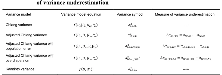
Table 1: Variance models and their associated variance symbols and measures of variance underestimation
Variance model Variance model equation Variance symbol Measure of variance underestimation
Chiang variance 𝑓(𝐷𝑥|𝑃𝑥,𝐷𝑤,𝑃𝑤) 𝜎𝐿𝐸2.𝐶ℎ ---
Adjusted Chiang variance 𝑓(𝐷𝑥,𝐷𝑤|𝑃𝑥,𝑃𝑤) 𝜎𝐿𝐸2.𝑎𝑑𝑗 ∆𝜎𝑎𝑑𝑗.𝐶ℎ=𝜎𝐿𝐸.𝑎𝑑𝑗− 𝜎𝐿𝐸.𝐶ℎ
Adjusted Chiang variance with
population error 𝑓(𝐷𝑥,𝐷𝑤,𝑃𝑤|𝑃𝑥) 𝜎𝐿𝐸2.𝑎𝑑𝑗.𝑝𝑜𝑝 ∆𝜎𝑝𝑜𝑝.𝑎𝑑𝑗=𝜎𝐿𝐸.𝑎𝑑𝑗.𝑝𝑜𝑝− 𝜎𝐿𝐸.𝑎𝑑𝑗
Adjusted Chiang variance with
overdispersion 𝑓(𝐷𝑥,𝐷𝑤|𝑃𝑥,𝑃𝑤) 𝜎𝐿𝐸2.𝑎𝑑𝑗.𝑁𝐵7 ∆𝜎𝑎𝑑𝑗.𝐶ℎ.𝑁𝐵=𝜎𝐿𝐸.𝑎𝑑𝑗.𝑁𝐵− 𝜎𝐿𝐸.𝐶ℎ.𝑁𝐵
Kannisto variance 𝑓(𝐷𝑥|𝑃𝑥) 𝜎𝐿𝐸2.𝐾𝑛 ---
2.2 The ‘standard’ Chiang variance model
In Chiang’s derivation of the LE variance (Chiang 1984), the age-specific death counts are considered the only sources of statistical variability. The variance contribution of the last age interval is completely omitted, however, leading to the following variance model:
𝐿𝐸𝐶ℎ =𝑓(𝐷𝑥|𝑃𝑥,𝐷𝑤,𝑃𝑤), where 𝐷𝑥 and 𝑃𝑥 are the age-specific death and population
counts corresponding to age group 𝑥= 0 …w-1, and 𝐷𝑤 and 𝑃𝑤 are the death and
population counts for the last, 𝑤𝑡ℎ, age interval. The delta method expression for the
standard Chiang variance is thus 𝜎𝐿𝐸2.𝐶ℎ≈ ∑ �𝜕𝐿𝐸𝜕𝐷𝑥� 2
𝜎𝐷2𝑥
𝑤−1
𝑥=0 . Under the assumption that
the death counts are distributed binomially, Chiang derived tractable expressions for the partial derivative weights to obtain the well-known expression for the LE variance:
𝜎𝐿𝐸2.𝐶ℎ≈ �(𝑝0𝑥)2[(1− 𝑎𝑥)𝑛𝑥+𝐿𝐸𝑥+1]2�𝑞𝑥 2(1− 𝑞
𝑥)
𝐷𝑥 �
𝑤−1
𝑥=0
, (1)
where 𝑝0𝑥 is the survival probability from age 0 to age 𝑥, 𝑎𝑥 is the fraction of age
interval lived, 𝑛𝑥 is the width of the age interval, 𝐿𝐸𝑥+1 is the life expectancy from age
𝑥+ 1, and 𝑞𝑥 is the probability of dying in age interval 𝑥. Equation 1 represents the
only available analytic formula for the 𝐿𝐸 variance and has been widely used in studies of LE to estimate its precision and for statistical testing (von Gaudecker and Scholz 2007; Geruso 2012; Kyte and Wells 2010; Stratton et al. 2012). It is evident from this
7 The subscript ‘NB’ will be used to denote the LE variance with overdispersion; ‘NB’ refers to the negative
equation, however, that the Chiang LE variance represents the sum of variance contributions corresponding to each age interval except the last.
2.3 The ‘adjusted’ Chiang LE variance model
The life table closure method of the Chiang LE estimator assumes that the mortality or hazard rate in the last age interval is constant in time, which results in the following estimate of the person-years contributed: 𝐿𝑤=ℓ𝑤/𝑀𝑤=ℓ𝑤𝑃𝑤/𝐷𝑤, where ℓ𝑤
represents the number of survivors at the beginning of the last age interval, and
𝑀𝑤=𝐷𝑤/𝑃𝑤 represents the mortality rate of the last age interval. As first noted in
2001 (Silcocks, Jenner, and Reza 2001), however, this dependence of 𝐿𝐸 on 𝐷𝑤 entails
that its variance contribution should also be accounted for. The corrected variance model for the Chiang LE is then 𝐿𝐸𝑎𝑑𝑗=𝑓(𝐷𝑥,𝐷𝑤|𝑃𝑥,𝑃𝑤). Application of the delta
method and using a Poisson distribution for 𝐷𝑤 yields the following corrected LE
variance formula, which has been termed the ‘adjusted’ Chiang variance in previous studies (Eayres and Williams 2004; Toson and Baker 2003) (cf. Appendix 1 for further details):
𝜎𝐿𝐸2.𝑎𝑑𝑗≈ � �𝜕𝐿𝐸𝜕𝐷 𝑥�
2
𝜎𝐷2𝑥+
𝑤−1
𝑥=0
�𝜕𝐿𝐸 𝜕𝐷𝑤�
2
𝜎𝐷2𝑤.
The second term in this equation represents the variance contribution of the last age interval death count. Assuming 𝐷𝑤 is Poisson distributed such that 𝜎𝐷2𝑤=𝐷𝑤, and
substituting the expression for 𝐿𝑤 yields for the correction term (cf. Appendix 1 for
further details):
�𝜕𝐿𝐸𝜕𝐷
𝑤� 2
𝜎𝐷2𝑤=� 𝜕 𝜕𝐷𝑤�
𝐿𝑤
ℓ0�� 2
𝐷𝑤=�𝜕𝐷𝜕 𝑤�
𝑃𝑤
𝐷𝑤𝑝0𝑤�� 2
𝐷𝑤= 𝑝0𝑤 2
𝑀𝑤3𝑃𝑤
Therefore,
𝜎𝐿𝐸2.𝑎𝑑𝑗≈ 𝜎𝐿𝐸2.𝐶ℎ+ 𝑝0𝑤
2
𝑀𝑤3𝑃𝑤. (2)
The following key aspects can be noted: 𝜎𝐿𝐸2.𝑎𝑑𝑗 is readily estimated by first
computing the standard Chiang variance and then adding a correction term, 𝜎𝐿𝐸2.𝑎𝑑𝑗 >
𝜎𝐿𝐸2.𝐶ℎ, and therefore the standard Chiang variance always underestimates the ‘correct’
probability 𝑝0𝑤 but decreases with increasing mortality rate 𝑀𝑤 and population 𝑃𝑤 of
the last age interval.
2.4 The adjusted Chiang LE variance model with population error
In the statistical analysis of mortality rate metrics, the population or denominator counts are generally assumed to have negligible variability as compared to the death or numerator counts. However, this assumption may be untenable for the last age interval, which comprises the oldest age category of the population, and for which numerous data uncertainty issues have been raised. Identified sources of error include: age exaggeration and underestimation, age heaping, and transcription error (Coale and Kisker 1990). These considerations motivate the following variance model, which includes the variance of population counts of the last age interval: 𝐿𝐸𝑎𝑑𝑗.𝑝𝑜𝑝 =
𝑓(𝐷𝑥,𝐷𝑤,𝑃𝑤|𝑃𝑥). The delta method expression for this variance model is as follows:
𝜎𝐿𝐸2.𝑎𝑑𝑗.𝑝𝑜𝑝≈ � �𝜕𝐿𝐸𝜕𝐷 𝑥�
2
𝜎𝐷2𝑥+
𝑤−1
𝑥=0
�𝜕𝐷𝜕𝐿𝐸
𝑤� 2
𝜎𝐷2𝑤+� 𝜕𝐿𝐸 𝜕𝑃𝑤�
2
𝜎𝑃2𝑤
Detailed assessments of Canadian data using the ‘extinct generation’ method (Bourbeau and Lebel 2000) indicate a proportional population data error of approximately ±5% in the 90+ age group (cf. Appendix 1, Section 3). This results in a population variance estimate of 𝜎𝑃2𝑤≈ �
0.05 2 𝑃𝑤�
2
. Using the estimate for 𝜎𝑃2𝑤 and
substituting the expression for 𝐿𝑤 yields for this correction term (cf. Appendix 1,
Section 3 for further details):
�𝜕𝐿𝐸𝜕𝑃
𝑤� 2
𝜎𝑃2𝑤=� 𝜕 𝜕𝑃𝑤�
𝑃𝑤
𝐷𝑤𝑝0𝑤�� 2
�0.052 𝑃𝑤� 2
=�𝑝𝐷0𝑤
𝑤� 2
�0.052 𝑃𝑤� 2
=�𝑝𝑀0𝑤
𝑤� 2
�0.052 �
2
Therefore,
𝜎𝐿𝐸2.𝑎𝑑𝑗.𝑝𝑜𝑝≈ 𝜎𝐿𝐸2.𝑎𝑑𝑗+�𝑝𝑀0𝑤 𝑤�
2
�0.052 �2 (3)
2.5 The adjusted Chiang LE variance with overdispersion
The 𝐿𝐸 variance model in the presence of overdispersion is identical to that of the adjusted Chiang case, since the sources of stochastic variability remains that of the age-specific death count. Thus 𝐿𝐸𝑎𝑑𝑗.𝑁𝐵=𝑓(𝐷𝑥,𝐷𝑤|𝑃𝑥,𝑃𝑤). For the purpose of testing the
effect of overdispersion a specific and standard parameterization of the negative binomial (𝑁𝐵) distribution will be used, where age-specific death counts (𝐷𝑥) are
interpreted as the number of events occurring, conditional on a specified probability of death (𝑞𝑥) and number of survivors at the end of the age interval (denoted 𝑃𝑥+)
(DeGroot 1986; Lloyd-Smith 2007; Manton and Stallard 1981). For 𝑥<𝑤, the variance of the death count can be readily expressed in terms of the standard binomial variance 𝜎𝐷2𝑥 and the estimated populations at the start (𝑃𝑥−) and end (𝑃𝑥+) of the interval
(cf. Appendix 1, Section 4): 𝜎𝐷2𝑥.𝑁𝐵=𝐷𝑥�
𝑃𝑥−
𝑃𝑥+�=�
𝑃𝑥−
𝑃𝑥+�
2
𝜎𝐷2𝑥. For the last age interval, 𝐷𝑥 is interpreted as the number of deaths that occur over an ‘observation’ period of 5
years (= the number of years of data aggregation). For this interval, 𝜎𝐷𝑤2 .𝑁𝐵=
𝐷𝑤�𝑃𝑤
−
𝑃𝑤+�=�
𝑃𝑤−
𝑃𝑤+� 𝜎𝐷𝑤
2 can be written (cf. Appendix 1, Section 4). The 𝐿𝐸variance in the
presence of overdispersion and including the contribution of the last age interval is thus:
𝜎𝐿𝐸2.𝑎𝑑𝑗.𝑁𝐵≈ � �𝜕𝐿𝐸𝜕𝐷 𝑥�
2
𝜎𝐷2𝑥.𝑁𝐵
𝑤−1
𝑥=0
+�𝜕𝐷𝜕𝐿𝐸
𝑤� 2
𝜎𝐷2𝑤.𝑁𝐵
=�(𝑝0𝑥)2[(1− 𝑎𝑥)𝑛𝑥+𝐿𝐸𝑥+1]2𝑞𝑥 2(1− 𝑞
𝑥) 𝐷𝑥 � 𝑃𝑥− 𝑃𝑥+� 2 𝑤−1 𝑥=0
+ 𝑝0𝑤2
𝑀𝑤3𝑃𝑤�
𝑃𝑤−
𝑃𝑤+� (4)
=𝜎𝐿𝐸2.𝐶ℎ.𝑁𝐵+ 𝑝0𝑤 2
𝑀𝑤3𝑃𝑤�
𝑃𝑤−
𝑃𝑤+�,
where Equations 1 and 2 have been used with the binomial variances replaced by their overdispersed counterparts. As 𝑃𝑥−>𝑃𝑥+, Equation 4 shows that overdispersion will
inflate each of the component variance contributions to the total LE variance. Also, note that the ratio 𝑃𝑥−/𝑃𝑥+ results in an increasing variance inflation effect with age,
2.6 The variance model of the Kannisto extrapolation closure method
A detailed empirical study (Thatcher, Kannisto, and Vaupel 1998) has shown that the logistic or ‘Kannisto’ function accurately describes the mortality rates at the highest ages (80-104 years), overcoming the observed lack of fit of the classical Gompertz function at these ages. Thus the Kannisto extrapolation method fits the logistic function to the age-specific life table mortality rates: 𝜇(𝑥) =∝ 𝑒𝛽𝑥/(1+∝ 𝑒𝛽𝑥). The coefficients
∝,𝛽 are estimated by regression fitting to the age intervals preceding the last, and the function 𝜇(𝑥) is then extrapolated to estimate the mortality rate profile over the last age interval. The life-years contribution to the LE, which represents the closure method, can then be estimated using standard demographic theory: 𝐿𝑤=ℓℓ𝑤0∫ 𝑒𝑥𝑝 �− ∫ 𝜇𝑥∞𝑤 𝑥𝑥𝑤 (𝑦)𝑑𝑦�𝑑𝑥.
The variance model for the Kannisto closure method is 𝐿𝐸=𝑓(𝐷𝑥|𝑃𝑥), 𝑥=
0 …𝑤 −1, where fitting of data from preceding age intervals has removed any dependence of the 𝐿𝐸 on data from the last age interval. An analytic expression for
𝜎𝐿𝐸2.𝐾𝑛 is not possible due to the complex dependence of the life years in the last age
interval, 𝐿𝑤, on the mortality rates 𝐷𝑥 of the preceding age intervals. Therefore in this
study the variance of LE using the Kannisto closure method, 𝜎𝐿𝐸2.𝐾𝑛, is estimated using
Monte Carlo simulation, with binomial variances used for 𝜎𝐷2𝑥.
3. Data sources and methods
LE variance models were assessed using empirical life table data that spanned three subnational geographic scales: provincial, provincial or regional, and intra-regional; all resulting population strata were above the 5,000 PY threshold in size, as can be seen in Table 2. The provinces and territories of Canada contribute 248 ‘provincial’ and sex-specific strata ranging in size from 78,510‒31,880,000 PY (median=2,440,000 PY); life table data were obtained from the Canadian Human Mortality Database (CHMD 2015), aggregated over the years 2004‒2008. Stratification over the 18 health administrative regions of Quebec and by sex results in 36 regional strata ranging in size from 26,960‒4,794,000 PY (median=807,600 PY). Geographical maps showing the provinces and territories of Canada and the health administrative regions of Quebec are presented in Figures 1a and 1b.
8 Canada comprises 10 provinces and 3 territories; data from the Northwest Territories and Nunavut are
Table 2: Total age-aggregated population sizes (in numbers and person-years (PY)) of the three empirical datasets
Population size (Numbers and person‒years)
Dataset # strata Minimum Median Maximum
Provincial 24 15,700 (78,500 PY) 488,000 (2,440,000 PY) 6,376,000 (31,880,000 PY)
Regional 36 5,344 (26,720 PY) 161,520 (807,600 PY) 958,800 (4,794,000 PY)
Intra-regional 231 1,573 (7,865 PY) 45,220 (226,100 PY) 460,200 (2,301,000 PY)
Further stratification by tertiles defined on the 25th and 75th percentiles of material and social deprivation (Pampalon et al. 2012), including the combined extremes of each dimension, were done resulting in 231 intra-regional strata9 ranging in size from 7,865‒2,301,000 PY (median=226,100 PY). For the regional and intra-regional life tables, death counts were extracted from the Quebec health ministry vital statistics files, while population counts for the middle year of the period were obtained from 2006 census data and adjusted for under-enumeration (Pelletier 2005; Statistics Canada 2006); the first age interval mortality rate is estimated by the ratio of deaths to the number of live births (Brown 1993). Life tables were calculated using the Chiang method (Chiang 1984); in the implementation of the Kannisto closure method, the Chiang method was used to estimate the life years contributed for all age intervals except the last. Five-year age intervals were used except for the first (0‒1) and last (90+) intervals. For the first age interval, the fraction of interval lived was set to 0.1. All life table and subsequent statistical analyses were done using R (version 2.15) statistical software.
9 Regions 10, 17, and 18 are excluded here due to their smaller population size, as well as 9 strata for which
Figure 1b): The 18 health administrative regions of Quebec
The difference in LE standard error with and without a particular variance contribution of the last age interval is termed ∆𝜎 (=𝜎𝑐𝑜𝑟𝑟𝑒𝑐𝑡𝑒𝑑− 𝜎𝑢𝑛𝑐𝑜𝑟𝑟𝑒𝑐𝑡𝑒𝑑) and
variance correction relative to the absolute magnitude of the LE standard error, and to provide comparison of corrected vs. uncorrected standard error magnitudes.
The global impact of the last age interval variance corrections is estimated using the prevalence at which elevated ∆𝜎 occurs over the 3 empirical datasets using two thresholds: ∆𝜎 > 0.02 and ∆𝜎 > 0.1. The former threshold was established by Toson and Baker (Toson and Baker 2003) and will be critically re-evaluated in the current study; the latter threshold represents a more liberal value that corresponds to a substantial increase in LE confidence interval coverage of approximately 0.4 years.
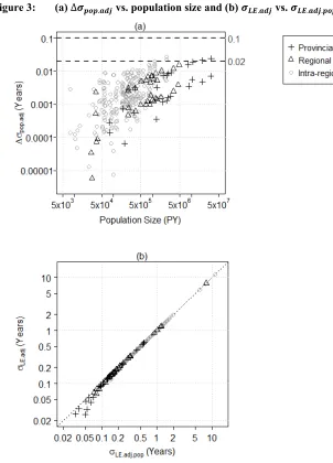
The false positive rate (or type 1 error rate) (Gravetter and Wallnau 2002) measures the increase in the number of erroneous statistical test results that occur due to the omission of a last age interval variance component (and concomitant underestimation of the standard error of the LE estimator). It equals the ratio of the number of false positives to the total number of statistical tests performed, when an ‘uncorrected’ variance formula is used relative to a ‘corrected’ one. False positive rates are estimated using statistical tests done in each of the three datasets, which comprise: tests of LE differences relative to the Canadian average in provincial-level strata, tests of LE differences relative to the Quebec average in regional strata, and tests of LE inequalities via comparison of LE between extremes (i.e., high vs. low) of material, social, and combined deprivation tertiles in intra-regional strata. Two significance levels or nominal false positive rates, α = 0.05 (or 5%) and α = 0.01 (or 1%), are considered: the former represents a standard significance level, while the latter represents a frequently used, more conservative level.
4. Results
4.1 The adjusted Chiang variance model
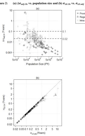
Figure 2a shows ∆𝜎𝑎𝑑𝑗.𝐶ℎ=𝜎𝐿𝐸.𝑎𝑑𝑗− 𝜎𝐿𝐸.𝐶ℎ plotted vs. population size for the adjusted
Chiang variance model. Crosses, triangles, and gray circles represent results for the provincial, regional, and intra-regional strata respectively, while the dashed lines indicate the 0.02 and 0.1 threshold values. The prevalence of ∆𝜎𝑎𝑑𝑗.𝐶ℎ exceeding these
two thresholds is also presented in Table 3a.
Overall, it can be seen that the last age interval can contribute substantially to the LE variance. Approximately 49% of strata exhibit ∆𝜎𝑎𝑑𝑗.𝐶ℎ higher than the 0.02 upper
limit (cf. Table 3a) reported in previous studies by Toson and Baker, despite all strata exceeding 5,000 PY in size. ∆𝜎𝑎𝑑𝑗.𝐶ℎ frequently attains values greater than 0.1 years,
with several extreme values found near 7 years, as reflected by a prevalence of ≈9% of
Figure 2a shows an increasing trend for ∆𝜎𝑎𝑑𝑗.𝐶ℎ with decreasing population size,
though considerable variability in the results prevents establishment of a clear threshold that would reliably classify strata into low vs. high ∆𝜎𝑎𝑑𝑗.𝐶ℎ, especially over regional
and sub-regional strata. This trend with population size is also evidenced in Table 3a, which shows that the prevalence of elevated ∆𝜎𝑎𝑑𝑗.𝐶ℎ increases with decreasing
geographic scale, from 4.2% to 58.4% corresponding to ∆𝜎𝑎𝑑𝑗.𝐶ℎ > 0.02, and from 0.0%
to 10.4% corresponding to ∆𝜎𝑎𝑑𝑗.𝐶ℎ > 0.1. ∆𝜎𝑎𝑑𝑗.𝐶ℎ also exhibited general scaling trends
when plotted against a range of other key life table parameters, though no clear classification thresholds could be identified here either (cf. Appendix 2).10
Figure 2b shows the scatterplot of the standard Chiang vs. adjusted Chiang standard errors. The adjusted Chiang standard error varies greatly in size, from ≈0.03 to 11 years, reflecting the range of population sizes and LE magnitudes spanned by the empirical datasets. The magnitude of the last age interval variance contribution is represented by the rightward shift in data points from the 1‒1 (dotted) line. It can be seen that for many strata, especially from the intra-regional dataset, there is a sizeable last age interval variance contribution relative to the magnitude of the LE standard error. This contribution tends to increase with increasing SE with notably large contributions of ∆𝜎𝑎𝑑𝑗.𝐶ℎ ≈1‒10 years occurring in the LE estimates with the largest
standard errors.
Table 3b lists the false positive rates that result from use of the standard Chiang variance relative to the adjusted Chiang variance, for the statistical tests previously described, over the 3 datasets. Use of the standard Chiang variance results in substantial overall increases in false positive rates of 4.9% and 4.2% over nominal false positive rates of α = 0.05 (5%) and α = 0.01 (1%), respectively. No false positives occurred in statistical tests done in the province-level strata, while the rates for the region-level strata were 5.6% and 5.6% for α = 0.05 and 0.01, and those for the intra-regional strata were 4.8% and 6.0% respectively.
10 Note that due to the tight correspondence between population size and LE standard error, scaling trends
Table 3a): Proportion of strata with elevated ∆𝝈𝒂𝒅𝒋.𝑪𝒉
Dataset # of Strata % Δσadj.Ch > 0.02 % Δσadj.Ch > 0.1
Provincial 24 4.2% (1/24) 0.0% (0/24)
Regional 36 13.9% (5/36) 2.8% (1/36)
Intra-regional 231 58.4% (135/231) 10.4% (24/231)
Total 291 48.5% (141/291) 8.6% (25/291)
Table 3b): Induced false positive rates for 𝝈𝑳𝑬𝟐 .𝑪𝒉 with respect to 𝝈𝑳𝑬𝟐 .𝒂𝒅𝒋
# of Statistical False positive False positive
Dataset Comparisons rate, α=0.05 rate, α=0.01
Provincial 24 0.0% (0/24) 0.0% (0/24)
Regional 36 5.6% (2/36) 5.6% (2/36)
Intra-regional 83 4.8% (4/83) 6.0% (5/83)
4.2 The adjusted Chiang variance model with population error
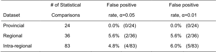
∆𝜎𝑝𝑜𝑝.𝑎𝑑𝑗 =𝜎𝐿𝐸.𝑎𝑑𝑗.𝑝𝑜𝑝− 𝜎𝐿𝐸.𝑎𝑑𝑗, shown plotted in Figure 3a, represents the
incremental variance contribution of population error in the last age interval, relative to the adjusted Chiang variance, estimated over the 3 datasets. In contrast to ∆𝜎𝑎𝑑𝑗.𝐶ℎ,
∆𝜎𝑝𝑜𝑝.𝑎𝑑𝑗 increases with population size due to the proportional dependence of the
population variance on 𝑃𝑤 as indicated by the last term in Equation 3. Overall, however,
the magnitude of ∆𝜎𝑝𝑜𝑝.𝑎𝑑𝑗 is relatively small, reaching an upper limit of ≈0.02 years
only when 𝑃𝑡𝑡𝑙 exceeds 1.5×10⁶ PY. As shown in Table 4a, the prevalence of
∆𝜎𝑝𝑜𝑝.𝑎𝑑𝑗>0.02 is 1.7%, indicating that for a relatively small number of cases, only a
slight increase in LE standard errors over that of ∆𝜎𝑎𝑑𝑗.𝐶ℎ occurs, with the largest strata
from the provincial and intra-regional datasets contributing these additional cases. Inclusion of population error results in no cases with ∆𝜎𝑝𝑜𝑝.𝑎𝑑𝑗>0.1.
Figure 3b shows the adjusted Chiang standard error (𝜎𝐿𝐸.𝑎𝑑𝑗) plotted against the
adjusted Chiang standard error with population error included (𝜎𝐿𝐸.𝑎𝑑𝑗.𝑝𝑜𝑝). It can be
seen that the incremental contribution of population error is negligible except in the case of the largest population strata (𝑃𝑡𝑡𝑙 ≳1.5×10⁶ PY) where the pre-existing small
population error results in a slight incremental impact on statistical tests, with a 1.4% increase in false positive rates relative to the adjusted Chiang variance model, as shown in Table 4b.
Table 4a): Proportion of strata with elevated ∆𝝈𝒑𝒐𝒑.𝒂𝒅𝒋
Dataset # of Strata % Δσpop.adj > 0.02 % Δσpop.adj > 0.1
Provincial 24 8.3% (2/24) 0.0% (0/24)
Regional 36 0.0% (0/36) 0.0% (0/36)
Intra-regional 231 1.3% (3/231) 0.0% (0/231)
Total 291 1.7% (5/291) 0.0% (0/291)
Table 4b): Induced false positive rates for 𝝈𝑳𝑬𝟐 .𝒂𝒅𝒋 with respect to 𝝈𝑳𝑬𝟐 .𝒂𝒅𝒋.𝒑𝒐𝒑
# of Statistical False positive False positive
Dataset Comparisons rate, α=0.05 rate, α=0.01
Provincial 24 8.3% (2/22) 0.0% (0/20)
Regional 36 0.0% (0/26) 2.8% (1/24)
Intra-regional 83 0.0% (0/53) 1.2% (1/46)
Total 143 1.4% (2/101) 1.4% (2/90)
4.3 The last age interval variance contribution in the presence of overdispersion
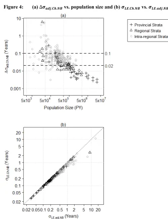
Figure 4a shows the variance contribution of the last age interval in the presence of overdispersion (∆𝜎𝑎𝑑𝑗.𝐶ℎ.𝑁𝐵 =𝜎𝐿𝐸.𝑎𝑑𝑗.𝑁𝐵− 𝜎𝐿𝐸.𝐶ℎ.𝑁𝐵) plotted vs. population size. The
magnitude of ∆𝜎𝑎𝑑𝑗.𝐶ℎ.𝑁𝐵 is in general higher than that of its non-overdispersed
counterpart ∆𝜎𝑎𝑑𝑗.𝐶ℎ, due to the 𝑃𝑤−⁄𝑃𝑤+ factor contributed mathematically by
overdispersion in the last age interval. This is reflected in the markedly higher overall prevalences of 80.1% of ∆𝜎𝑎𝑑𝑗.𝐶ℎ.𝑁𝐵 > 0.02 and 19.9% of ∆𝜎𝑎𝑑𝑗.𝐶ℎ.𝑁𝐵 > 0.1 (cf. Table
5a).
∆𝜎𝑎𝑑𝑗.𝐶ℎ.𝑁𝐵 decreases with increasing population size, following trends that
resemble closely those of ∆𝜎𝑎𝑑𝑗.𝐶ℎ. The prevalence of elevated ∆𝜎𝑎𝑑𝑗.𝐶ℎ.𝑁𝐵 also
increases throughout the three datasets with decreasing population size, from 16.7% to 91.3% for ∆𝜎𝑎𝑑𝑗.𝐶ℎ.𝑁𝐵 > 0.02, and from 8.3% to 22.5% for ∆𝜎𝑎𝑑𝑗.𝐶ℎ.𝑁𝐵 > 0.1 (cf. Table
5a).
The scatterplot of 𝜎𝐿𝐸.𝑎𝑑𝑗.𝑁𝐵 vs. 𝜎𝐿𝐸.𝐶ℎ.𝑁𝐵 in Figure 4b illustrates that the size of
has thus been amplified by overdispersion. ∆𝜎𝑎𝑑𝑗.𝐶ℎ.𝑁𝐵 is also proportionately larger
overall, as shown by the more pronounced rightward shift in points from the dotted black (1‒1) line.
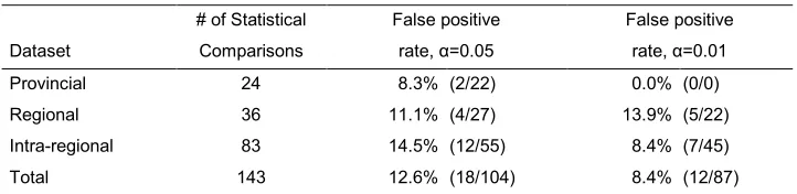
Table 5b (in comparison with Table 3b) shows that the impact of the last age interval variance on statistical tests is further amplified in the presence of overdispersion. This is evidenced by substantially higher increases in false positive rates by 12.6% and 8.4% with respect to nominal false positive rates or significance levels of 0.05 (5%) and 0.01 (1%), respectively. This overall increase in false positive rates is produced by corresponding increases in virtually all dataset and α combinations, which show increases in false positive rates ranging up to 14.5%.
Table 5a): Proportion of strata with elevated ∆𝝈𝒂𝒅𝒋.𝑪𝒉.𝑵𝑩
Dataset # of Strata % Δσadj.Ch.NB > 0.02 % Δσadj.Ch.NB > 0.1
Provincial 24 16.7% (4/24) 8.3% (2/24)
Regional 36 50.0% (18/36) 11.1% (4/36)
Intra-regional 231 91.3% (211/231) 22.5% (52/231)
Total 291 80.1% (233/291) 19.9% (58/291)
Table 5b): Induced false positive rates for 𝝈𝑳𝑬𝟐 .𝒂𝒅𝒋.𝑵𝑩 with respect to 𝝈𝑳𝑬𝟐 .𝑪𝒉.𝑵𝑩
# of Statistical False positive False positive
Dataset Comparisons rate, α=0.05 rate, α=0.01
Provincial 24 8.3% (2/22) 0.0% (0/0)
Regional 36 11.1% (4/27) 13.9% (5/22)
Intra-regional 83 14.5% (12/55) 8.4% (7/45)
Total 143 12.6% (18/104) 8.4% (12/87)
4.4 Comparative performance of the Kannisto extrapolation closure method
Closure of the life table with the Kannisto extrapolation procedure results in an LE estimator that is no longer equivalent to the Chiang LE. Thus the resulting Kannisto LE variance cannot be represented as an additive variance contribution to the standard Chiang variance, as was done for the other variance models tested. However, the performance of the Kannisto LE variance can be roughly assessed through scatterplots of the Kannisto LE standard error, 𝜎𝐿𝐸.𝐾𝑛, vs. the adjusted Chiang standard error,
𝜎𝐿𝐸.𝑎𝑑𝑗. Figure 5a shows 𝜎𝐿𝐸.𝐾𝑛 vs. 𝜎𝐿𝐸.𝑎𝑑𝑗 for the subset of cases in which
∆𝜎𝑎𝑑𝑗.𝐶ℎ>0.1 and in which there is an elevated variance contribution of the last age
variance contribution of the last age interval, as indicated by the overall rightward shift in points from the dashed (1‒1) line in the Figure. In particular, substantial reductions in standard error of up to ≈10 years occur when 𝜎𝐿𝐸.𝑎𝑑𝑗 becomes large (>1). Figure 5b
shows that for ∆𝜎𝑎𝑑𝑗.𝐶ℎ<0.1, 𝜎𝐿𝐸.𝐾𝑛 is comparable to 𝜎𝐿𝐸.𝑎𝑑𝑗, which is expected since
the variance contribution of the last age interval is already small.
Figure 5: 𝝈𝑳𝑬.𝑲𝒏 vs. 𝝈𝑳𝑬.𝒂𝒅𝒋 for (a) ∆𝝈𝒂𝒅𝒋.𝑪𝒉≥ 𝟎.𝟏 and (b) ∆𝝈𝒂𝒅𝒋.𝑪𝒉<𝟎.111
11 Results have been ‘split’ by level of ∆𝜎
5. Discussion
The current study demonstrates that the last age interval can contribute substantially to the LE variance when using the Chiang LE estimator. It is firstly shown that inclusion of the variance contribution of the last age interval mortality count can lead to increases in the LE standard error that greatly exceed the previously reported 0.02 upper limit (Toson and Baker 2003), even for populations substantially larger than 5,000 PY. It is further demonstrated that overestimation of the precision of LE is widespread and leads to the substantial inflation of false discovery rates or type 1 error in statistical comparisons at subnational scales.
Assessment of an extended variance model indicates that population error in the last age interval contributes negligibly to the LE variance for population sizes below 1.5 x 10⁶ PY. For populations > 1.5 x 10⁶ PY, population error can make a proportionately substantial contribution to the total variance, although the absolute variance contribution remains small (< 0.03 years). In light of these results and of the likely improvements in population data quality since 1971‒1991 (from which conservative estimates of a 5% proportional error in population counts were derived), it is likely that the population error of the last age interval can be neglected for purposes of LE variance estimation. Despite representing a known and major source of error, assessment of the last age interval population count error on LE variance has not previously been done. Our study addresses this gap in knowledge and provides a clear recommendation for practitioners.
The variance contribution of the last age interval increases in the presence of overdispersion, leading to marked increases in both the prevalence of severe variance underestimation and inflated false positive rates when the uncorrected Chiang variance is used. Overdispersion, also known as heterogeneity or frailty, is likely present to some degree in most mortality data, and manifests in the observed mortality trends at the highest ages (Andreev and Bourbeau 2006; Bebbington, Lai, and Zitikis 2011; Ting, Yang, and Anderson 2013). Thus the overdispersed LE variance results of this study may represent a more realistic scenario, which further underscores the substantial impact of the last age interval on variance.
Inclusion of the variance contribution of the last age interval death count is thus found to be essential when using the Chiang LE estimator at subnational scales. The substantial overestimation of precision and false positives that results from use of the uncorrected Chiang LE variance can lead to errors that have both scientific and policy consequences. As reliable thresholds to classify population strata in regard to the expected magnitude of the last age interval variance are not possible, the mathematical correction of each LE variance estimate is recommended. To this end, the simple, additive formulae provided in this manuscript can be used by practitioners to readily correct existing or planned variance estimates. The Excel tool provided in this study demonstrates the implementation of each of these corrections on a sample life table, and is intended to further facilitate implementation.
To summarize the findings of our study for operational purposes, the adjusted Chiang variance (Equation 2, Section 2.3, 𝜎𝐿𝐸2.𝑎𝑑𝑗) should be used in place of the
standard Chiang formula for estimating the LE variance. The adjusted Chiang variance with overdispersion (Equation 4, Section 2.5, 𝜎𝐿𝐸2.𝑎𝑑𝑗.𝑁𝐵) is recommended when the
choice has already been made to model overdispersion in mortality counts in the other age intervals. The addition of population error (Section 2.3) is found to affect the LE variance negligibly and need not be used. The variance model of the Kannisto LE (Section 2.6) is valid but requires Monte Carlo simulation to evaluate, and applies only when the Kannisto life table closure method is used in place of the Chiang closure method.
5.1 Study limitations
Although tests were done on a wide range of empirical data, these data are not completely general and do not represent the full range of possible life tables. Nevertheless, the results are sufficient to demonstrate the substantial impact of the last age interval on LE variance, which is the principal objective of the study. Overall, the great variability in stratum-specific results observed in the current study, and the demonstrated inadequacy of the previously identified 0.02 limit (which was estimated from simulations of a single test population), underscore the need for empirical datasets when assessing the performance of life-table-based metrics.
Life table data were restricted to those of Canada (for province level analyses) and Quebec (for regional and intra-regional analyses), though these data are expected to be comparable to other developed nations. LE in fact varies quite widely (from 64.1 to 94.5 years) over strata, indicating a broad range of demographic conditions, some of which may resemble those of other countries at different stages of development. In particular, Figure A-2.1e illustrates that substantial variance underestimation may occur regardless of the magnitude of estimated LE, and thus indicates the likely importance of the last age interval for non-Canadian datasets.
In reality, the true or correct LE variance is inherently unknown, since LE can only be sampled or observed once for a given time period and population. Therefore the increase in false positive rate was estimated approximately by comparing statistical tests using ‘uncorrected’ vs. ‘corrected’ variances. This likely results in conservative estimates of false positive rate increase and thus of impact, since ‘corrected’ variances are likely underestimates of the true LE variance due to the presence of additional, unaccounted-for sources of variability. The hypothetical use of true LE variances would therefore tend to further increase the impact of the estimated LE variance corrections and thus further strengthen the conclusions the study. Overall, the ‘corrected’ LE variance formulae derived in this study account for the stochastic contribution of age-specific death counts according to established statistical theory (Brillinger 1986; Chiang 1960; Keyfitz 1966), and thus are expected to be reasonable estimates of the true LE variance.
Variability in the last age interval population counts (𝜎𝑃𝑤) is likely produced by
age misreporting and other sources of error, whose exact mechanisms and thus probability distributions are in fact largely unknown. Nevertheless, the finding that the impact of 𝜎𝑃𝑤 on the overall LE variance is likely negligible is both general and robust
compared with error in death counts. Using an empirically based 5% proportional error, it can be further demonstrated that the variance contribution of population counts becomes comparable to that of death counts only for very large (≈1.2×10⁶) population sizes, where the total LE variance is likely small. Finally, additional validation analyses have shown that the impact of population error remains negligible despite varying the assumed coverage associated with the observed empirical error, as well as consideration of corresponding ‘opposing’ population count error in younger age intervals. Detailed discussion and analyses of these issues are presented in Appendix 3.
The delta method utilizes a first order Taylor expansion of the function for which the variance is estimated. For this reason, the various derived expressions for variance are in fact first order approximations. However, validation studies that have compared the delta method standard error with Monte Carlo simulated standard errors have shown that the delta method is accurate (Eayres and Williams 2004). The delta method was used by Chiang in his original derivation of the LE variance (though the contribution the last age interval was neglected): it also sees widespread use for variance estimation in biostatistics in general (Cox 2005).
Performance of the Chiang LE variance was examined using a closure age of 90 years, which is the established norm in the Quebec Public Health Network (MSSS 2011) and ensures robust LE estimation over datasets that include small strata. At provincial or national scales, however, sufficiently large age-specific population sizes and data quality often permit LE estimation using elevated closure ages of up to 100 years or higher (CHMD 2015; Martel et al. 2012; Wilmoth et al. 2007). An increase in closure age to 100 years would result in a greatly reduced life table survival probability from birth to the last age interval (𝑝0𝑤), which would in turn reduce the magnitude of
the last age interval contribution to the LE variance (cf. Equation 2). Furthermore, due to the inverse scaling with population size, the absolute magnitudes of the total LE variance and the last age interval contribution become quite small. Thus it must be emphasized that the scope of the current study pertains to LE estimation at subnational scales (down to population sizes of 5,000 PY), where the LE variance is relatively substantial and closure ages of 90 years or less are typically used.
Conversely, reduction of the life table age to below 90 years could also represent a possible strategy to alleviate large variance contributions from the last age interval, by effectively increasing the last age interval population size and thereby reducing the frequency of sparse death counts. Validation tests show, however, that the last age interval variance contribution (∆𝜎𝐶ℎ.𝑎𝑑𝑗) remains substantial and widespread even when
substantial increase in excluded strata due to zero age-specific population counts or zero death counts in the last age interval for this case however12.
While a specific though widely used parameterization of the negative binomial distribution was used to describe heterogeneity in death counts, the actual degree of heterogeneity in real populations is unknown and difficult to estimate. However, the negative binomial parameterization used in the current study results in a variance inflation effect that increases with age, consistent with the expected increases in frailty in mortality rates due to survivorship effects (Vaupel, Manton, and Stallard 1979), and is thus a reasonable, representative model for heterogeneity. As a result, the general finding of the study ‒ that the impact of the last age interval on the LE variance is amplified in the presence of overdispersion ‒ is expected to hold for other realistic heterogeneity or frailty models.
Finally, the present study focuses on the variance properties of the Chiang LE estimator, which is but one of many existing LE estimators. It should be noted, however, that the Chiang closure method is identical to that used by numerous other classic LE methods including the ‘actuarial’, Greville, Sirken, Keyfitz-Frauenthal, and Schoen approaches (Greville 1943; Keyfitz and Frauenthal 1975; Schoen 1978; Siegel 2012). Thus the findings regarding the last age interval variance are applicable to a range of LE estimators. More generally, the Chiang method remains the most widely used and accessible procedure for the estimation of LE and its variance, and thus represents an important subject of study.
6. Conclusions
The present study represents the first detailed assessment of the variance properties of the last age interval and its impact on LE variance. The delta method framework has been extended to model population data error and mortality rate overdispersion properties of the underlying vital rates. Tests done on a range of empirical sub-national life table data demonstrate that the variance contribution of the last age interval can lead to severe underestimation of the total LE variance, as well as substantial increases in the false positive rate in statistical tests. It is hoped that this study will thus unambiguously demonstrate to practitioners and users the need to correct the standard Chiang LE variance. To facilitate implementation, accessible, additive correction formulae are provided for correcting the standard Chiang LE variance. Additionally, an Excel tool is provided that computes the life expectancy variances for all variance models (excepting the Kannisto) for a sample life table. The Chiang LE estimator is a widely accepted
12 Although methods (such as imputation) exist for dealing with these strata, examination of this issue is
standard for use by demographers, epidemiologists, and public health officers, due to its accessibility, ease of computation, robustness for smaller populations (≳ 5,000 PY), and available variance formula. It is hoped that the present study will contribute toward the improved validity of the numerous previous, ongoing, and future analyses done using this estimator.
7. Acknowledgements
References
Andreev, K.F. and Bourbeau, R. (2006). Frailty modeling of Canadian and Swedish mortality at adult and advanced ages. Unpublished manuscript.
Bajekal, M. (2005). Healthy life expectancy by area deprivation: Magnitude and trends in England, 1994‒1999. Health Statistics Quarterly 25: 18–27.
Bebbington, M., Lai, C.D., and Zitikis, R. (2011). Modelling deceleration in senescent mortality. Mathematical Population Studies 18(1): 18–37.doi:10.1080/0889848 0.2011.540173.
Bourbeau, R. and Desjardins, B. (2007). Mortality at extreme ages and data quality: The Canadian experience. In: Robine, J.-M., Crimmins, E.M., Horiuchi, S., Zeng, Y. (eds.). Human longevity, individual life duration, and growth of the oldest-old
population. Berlin: Springer: 167–185. doi:10.1007/978-1-4020-4848-7_8.
Bourbeau, R. and Lebel, A. (2000). Mortality statistics for the oldest-old: An evaluation of Canadian data. Demographic Research 2(2): doi:10.4054/demres.2000.2.2. Brillinger, D.R. (1986). The natural variability of vital rates and associated statistics.
Biometrics 42(4): 693–734.doi:10.2307/2530689.
Brown, R.L. (1993). Introduction to the mathematics of demography. New Hartford: ACTEX Publications.
Casella, G. and Berger, R.L. (2002). Statistical inference. Pacific Grove: Duxbury. Chiang, C.L. (1960). A stochastic study of the life table and its applications: II. Sample
variance of the observed expectation of life and other biometric functions.
Human Biology 32(3): 221–238.
Chiang, C.L. (1984). The life table and its applications. Malabar: Robert E. Krieger. CHMD (2015). Canadian Human Mortality Database [electronic resource].
http://www.bdlc.umontreal.ca/chmd/.
Coale, A.J. and Kisker, E.E. (1990). Defects in data on old-age mortality in the United States: New procedures for calculating mortality schedules and life tables at the highest ages. Asian and Pacific Population Forum 4(1): 1–32.
Cox, C. (2005). Delta method. In: Armitage, P. and Colton, T. (eds.). Encyclopedia of
biostatistics. New York: John Wiley: 1540–1542. doi:10.1002/0470011815.
b2a15029.
Eayres, D. and Williams, E.S. (2004). Evaluation of methodologies for small area life expectancy estimation. Journal of Epidemiology and Community Health 58: 243–249.doi:10.1136/jech.2003.009654.
Geronimus, A.T., Bound, J., Waidmann, T.A., Colen, C.G., and Steffick, D. (2001). Inequality in life expectancy, functional status, and active life expectancy across selected black and white populations in the United States. Demography 38(2): 227–251.
Geruso, M. (2012). Black-White disparities in life expectancy: How much can the standard SES variables explain? Demography 49(2): 553‒574.doi:10.1007/s13 524-011-0089-1.
Gravetter, F.J. and Wallnau, L.B. (2002). Essentials of statistics for the behavioral
sciences. Pacific Grove: Wadsworth.
Greville, T.N.E. (1943). Short methods of constructing abridged life tables. Record of
the American Institute of Actuaries 32(1): 29–42.
Horsman, J., Furlong, W., Feeny, D., and Torrance, G. (2003). The Health Utilities Index (HUI): Concepts, measurement properties and applications. Health and
Quality of Life Outcomes 1(54).doi:10.1186/1477-7525-1-54.
Keyfitz, N. (1966). Sampling variance of standardized mortality rates. Human Biology 38(3): 309–317.
Keyfitz, N. and Frauenthal, J. (1975). An improved life table method. Biometrics 31(4): 889–899.doi:10.2307/2529814.
Kyte, L. and Wells, C. (2010). Variations in life expectancy between rural and urban areas of England, 2001‒07. Health Statistics Quarterly 46: 25–50.
Lloyd-Smith, J.O. (2007). Maximum likelihood estimation of the negative binomial dispersion parameter for highly overdispersed data, with applications to infectious diseases. PLoS One 2(2): e180. doi:10.1371/journal.pone.0000180. Loukine, L., Waters, C., Choi, B.C., and Ellison, J. (2012). Impact of diabetes mellitus
on life expectancy and health-adjusted life expectancy in Canada. Population
Health Metrics 10(1): 7.
Manuel, D.G., Schultz, S.E., and Kopec, J.A. (2002). Measuring the health burden of chronic disease and injury using health adjusted life expectancy and the Health Utilities Index. Journal of Epidemiology and Community Health 56(11): 843– 850.
Martel, L., Provost, M., Lebel, A., Coulombe, S., and Sherk, A. (2012). Methods for
constructing life tables for Canada, provinces and territories. Statistics Canada.
Mathers, C. (1991). Health expectancies in Australia 1981 and 1988. Canberra: Australian Institute of Health.
Molla, M.T., Wagener, D.K., and Madans, J.H. (2001). Summary measures of population health: Methods for calculating healthy life expectancy. Healthy
People 2010, Statistical Notes (21): 1–11.
MSSS (2011). Pour guider l’action: Portrait de santé et de ses régions, les statistiques. Québec: Ministère de la Santé et des Services sociaux en collaboration avec l’Institut national de santé publique du Québec et l’Institut de la statistique du Québec.
Page, A., Begg, S., Taylor, R., and Lopez, A.D. (2007). Global comparative assessments of life expectancy: The impact of migration with reference to Australia. Bulletin of the World Health Organization 85(6): 474–481.
Pampalon, R., Hamel, D., Gamache, P., Philibert, M.D., Raymond, G., and Simpson, A. (2012). An area-based material and social deprivation index for public health in Québec and Canada. Canadian Journal of Public Health 103(Suppl 2): S17– S22.
Pelletier, G. (2005). La population du Québec par territoire des centres locaux de services communautaires, par territoire des réseaux locaux de services et par région sociosanitaire de 1981 à 2026. Québec : Santé et Services sociaux Québec.
http://www.santecom.qc.ca/BibliothequeVirtuelle/MSSS/2550450833.pdf. Robine, J.M., Romieu, I., and Cambois, E. (1999). Health expectancy indicators.
Bulletin of the World Health Organization 77(2): 181–185.
Scherbov, S. and Ediev, D. (2012). Significance of life table estimates for small populations: Simulation-based study of standard errors. Demographic Research 24(22): 527–550.doi:10.4054/DemRes.2011.24.22.
Schoen, R. (1978). Calculating life tables by estimating Chiang’s a from observed rates.
Demography 15(4): 625–635.doi:10.2307/2061212.
Shyrock, H.S. and Siegel, J.S. (1976). The methods and materials of demography. Abridged edition. New York: Academic Press.
Siegel, J.S. (2012). The life table. In: Siegel, J.S. The demography and epidemiology of
human health and aging. New York: Springer: 135–216.
doi:10.1007/978-94-007-1315-4_4.
Silcocks, P.B.S., Jenner, D.A., and Reza, R. (2001). Life expectancy as a summary of mortality in a population: Statistical considerations and suitability for use by health authorities. Journal of Epidemiology and Community Health 55: 38–43. doi:10.1136/jech.55.1.38.
Statistics Canada (2006). Census of population. http://www23.statcan.gc.ca/imdb/ p2SV.pl?Function=getSurvey&SDDS=3901&lang=en&db=imdb&adm=8&dis= 2.
Stratton, J., Mowat, D.L., Wilkins, R., and Tjepkema, M. (2012). Income disparities in life expectancy in the City of Toronto and Region of Peel, Ontario. Chronic
Diseases and Injuries in Canada 32(4): 208–215.
Sullivan, D.F. (1971). A single index of mortality and morbidity. HSMHA Health
Report 86(4): 347–354. doi:10.2307/4594169.
Thatcher, A.R., Kannisto, V., and Vaupel, J.W. (1998). The force of mortality at ages 80 to 120. In: Jeune, B. and Vaupel, J.W. (eds.). Odense Monographs on
Population Aging 5. Odense: Odense University Press.
Ting, L., Yang, C.Y., and Anderson, J.J. (2013). Mortality increase in late-middle and early-old age: Heterogeneity in death processes as a new explanation.
Demography 50(5): 1563–1591.doi:10.1007/s13524-013-0222-4.
Toson, B. and Baker, A. (2003). Life expectancy at birth: Methodological options for
small populations. Office for National Statistics.
Ver Hoef, J.M. (2012). Who invented the delta method? The American Statistician 66(2): 124–127.doi:10.1080/00031305.2012.687494.
Von Gaudecker, H.M. and Scholz, R.D. (2007). Differential mortality by lifetime earnings in Germany. Demographic Research 17(4): 83–108.doi:10.4054/Dem Res.2007.17.4.
Wilmoth, J.R., Andreev, D., Jdanov, D., and Glei, D.A. (2007). Methods protocol for
the human mortality database. Available at http://www.mortality.org/Public/
Docs/MethodsProtocol.pdf.
Wilmoth, J.R. and Lundstrom, H. (1996). Extreme longevity in five countries: Presentation of trends with special attention to issues of data quality. European
Appendix 1: Detailed derivation of variance formulae
In the following sections, formulae for LE variance are derived for the variance models examined in this study. Symbols for life table variables and indices follow the convention used in Chiang, which may differ slightly from standard demographic conventions, in order to facilitate comparison between the standard Chiang variance and the variance formulae of this study. All formulae are generally applicable to the variance of life expectancy from age ‘∝’. Thus for life expectancy from birth as presented in the main text, ∝= 0.
1. The standard Chiang variance model
The standard Chiang variance formula is shown below:
𝜎𝑒2𝛼=𝜎𝐶ℎ2∝=� 𝑝∝𝑥2 [(1− 𝑎𝑥)𝑛𝑥+𝑒𝑥+1]2 ×𝜎𝑝2𝑥
𝑤−1
𝑥=𝛼
, (A1.1)
where 𝑝∝𝑥 is the survival probability from age interval ∝ to age interval 𝑥, 𝑎𝑥 is the
fraction of age interval lived for age interval 𝑥, 𝑛𝑥 is the width (in years) of the age
interval, 𝑒𝑥+1 is the life expectancy from age 𝑥+ 1, and 𝜎𝑝2𝑥=𝑞𝑥2(1− 𝑞𝑥)/𝐷𝑥 is the
(binomial) variance of the survival probability 𝑝𝑥 for the 𝑥𝑡ℎ age interval.
For comparability with the other variance models in this study, the expression of the standard Chiang variance in terms of the variance of age-specific death counts is readily obtained: 𝑝𝑥= 1− 𝐷𝑥/𝑃𝑥− where 𝑃𝑥− is the population at the start of age
interval 𝑥 and is considered a constant with no statistical variability; thus 𝜎𝑝2𝑥= 𝜎𝐷2𝑥/𝑃𝑥−2 =𝜎𝐷2𝑥(𝑞𝑥/𝐷𝑥)2. Direct substitution into Equation A1.1 then yields:
𝜎𝑒2𝛼=𝜎𝐶ℎ2∝=� 𝑝∝𝑥2[(1− 𝑎𝑥)𝑛𝑥+𝑒𝑥+1]2 ×𝜎𝐷2𝑥� 𝑞𝑥
𝐷𝑥� 2 𝑤−1
𝑥=𝛼
, (A1.1a)
Overall, it can be seen that the Chiang LE variance is a weighted sum of the variance contributions of each age interval, with no contribution from the last (𝑤𝑡ℎ)
2. The ‘adjusted’ Chiang variance model
The derivation of the adjusted Chiang variance model is based closely on derivation of the standard Chiang LE variance and makes use of the same notation.
For the last age interval (𝑥=𝑤), the mortality rate or hazard is assumed to be constant in time, which leads to the standard Chiang closure method13 for the life-years lived in the last age interval:
𝐿𝑤=𝑀𝑙𝑤
𝑤
As life expectancy from age ∝ equals the sum over age intervals of the life-years lived divided by the starting population at age ∝ (𝑒∝=𝑙1∝∑𝑤𝑥=∝𝐿𝑥), the last age interval thus contributes the following additive term to the life expectancy:
1 ℓ𝛼𝐿𝑤= 1 ℓ𝛼 𝑙𝑤 𝑀𝑤= 𝑝𝛼𝑤 𝑀𝑤= 𝑃𝑤𝑝∝𝑤
𝐷𝑤 (A1.2)
The life expectancy variance, accounting for the contribution of the last age interval death count (𝐷𝑤), can then be expressed using the delta method in terms of the
known variances of 𝑝∝,𝑝∝+1, … ,𝑝𝑤−1,𝐷𝑤while noting that these variables are
statistically independent:
𝜎𝑒2𝛼=� � 𝜕𝑒∝
𝜕𝑝𝑥� 2 𝑤−1
𝑥=∝
𝜎𝑝2𝑥+� 𝜕𝑒∝
𝜕𝐷𝑤� 2
𝜎𝐷2𝑤 (A1.3)
Note that the first part of Equation A1.3 is identical to the standard variance equation (Chiang 1984) since the partial derivatives �𝜕𝑒∝
𝜕𝑝𝑥� are unaffected by 𝐷𝑤.
Therefore Equation A1.3 can be expressed as the sum of the standard Chiang variance and an additive correction term:
𝜎𝑒2𝛼 =𝜎𝐶ℎ2 +�
𝜕𝑒∝
𝜕𝐷𝑤�
2
𝜎𝐷2𝑤 (A1.4)
Using Equation A1.2 the partial derivative 𝜕𝑒∝
𝜕𝐷𝑤 is:
13 This closure method is also used by the ‘actuarial’, Greville, Sirken, Keyfitz and Frauenthal, and Schoen
𝜕𝑒𝛼 𝜕𝐷𝑤= 𝜕 𝜕𝐷𝑤� 𝑃𝑤𝑝∝𝑤 𝐷𝑤 �=− 𝑃𝑤𝑝∝𝑤
𝐷𝑤2 (A1.5)
Assuming a Poisson distribution for the number of deaths in the last age interval, the variance of the death count in the last age interval is:
𝜎𝐷2𝑤=𝐷𝑤 (A1.6)
Therefore the variance contribution term for the last age interval becomes:
�𝜕𝐷𝜕𝑒∝
𝑤� 2
𝜎𝐷2𝑤=� 𝑃𝑤𝑝∝𝑤
𝐷𝑤2 � 2
(𝐷𝑤) =𝑃𝑤 2𝑝
∝𝑤 2
𝐷𝑤3 =
𝑝∝𝑤2
𝑀𝑤3𝑃𝑤 (A1.7)
The final expression for the adjusted Chiang variance is thus:
𝜎𝑒2𝛼=𝜎𝐿𝐸2.𝑎𝑑𝑗=𝜎𝐶ℎ2∝+ 𝑝∝𝑤2
𝑀𝑤3𝑃𝑤 (A1.8)
For life expectancy from birth ∝= 0, and the adjusted Chiang variance is written:
𝜎𝑒20=𝜎𝐿𝐸2.𝑎𝑑𝑗=𝜎𝐶ℎ2 + 𝑝0𝑤2
𝑀𝑤3𝑃𝑤 (A1.9)
3. The adjusted Chiang variance model with error in population
counts
A delta method expansion, accounting for the additional contribution of population error in the last age interval, results in an additional variance contribution term to the adjusted Chiang variance:
𝜎𝑒2𝛼=� � 𝜕𝑒∝
𝜕𝑝𝑥� 2 𝑤−1
𝑥=∝
𝜎𝑝2𝑥+� 𝜕𝑒∝
𝜕𝐷𝑤� 2
𝜎𝐷2𝑤+� 𝜕𝑒∝
𝜕𝑃𝑤� 2
𝜎𝑃2𝑤
∴ 𝜎𝑒2𝛼=𝜎𝑎𝑑𝑗2 +� 𝜕𝑒∝
𝜕𝑃𝑤� 2
Bourbeau and Lebel (2000) (Table 3) provided estimates of the population error in Canadian data for the census years 1971, 1976, 1981, 1986, and 1991, for the age interval 90+, using the extinct generation method; both over-estimation and under-estimation of population counts were found. Based on these data, a +/‒ 5% proportional error in the population counts for the age interval 90+ was judged to be a reasonable approximation. Interpretation of this error estimate as a 95% confidence interval for a normally distributed variate leads to the following estimate for the variance of the last age interval population count:
2𝜎𝑃𝑤≈0.05𝑃𝑤 (A1.11)
∴ 𝜎𝑃𝑤2 ≈ �0.052 � 2
𝑃𝑤2 (A1.12)
Using equation A1.2, the partial derivative weight for the population count variance is: �𝜕𝑒𝜕𝑃∝ 𝑤� 2 =�𝜕𝑃𝜕 𝑤� 𝑃𝑤𝑝∝𝑤 𝐷𝑤 �� 2
=�𝑝𝐷0𝑤
𝑤� 2
(A1.13)
Therefore the incremental variance contribution due to population error is:
�𝜕𝑃𝜕𝑒𝛼
𝑤� 2
𝜎𝑃2𝑤=� 𝑃𝑤𝑝𝛼𝑤
𝐷𝑤 �
2
�0.052 �2 (A1.14)
For life expectancy from birth, ∝= 0 and the extended variance formula accounting for population error becomes:
𝜎𝑒20=𝜎𝐿𝐸2.𝑎𝑑𝑗.𝑝𝑜𝑝=𝜎𝐶ℎ2 + 𝑝0𝑤 2
𝑀𝑤3𝑃𝑤+�
𝑃𝑤𝑝0𝑤
𝐷𝑤 �
2
�0.052 �2=𝜎𝑎𝑑𝑗2 +�𝑃𝑤𝐷𝑝0𝑤 𝑤 �
2
4. The adjusted Chiang variance model in the presence of
overdispersion
A natural parameterization (Casella and Berger 2002; DeGroot 1986) of the negative binomial distribution is as follows:
𝐷𝑥~𝑁𝐵(𝑃𝑥+,𝑞𝑥), (A1.16) where the age-specific death counts are interpreted as the result of a sequence of Bernoulli trials such that 𝐷𝑥 deaths (successes) occur with probability 𝑞𝑥 for a given
number, 𝑃𝑥+, of survivors (failures). 𝑃𝑥+ is thus the number of survivors at the end of age
interval 𝑥, and 𝑞𝑥 is the probability of death for the age interval which can be written
𝐷𝑥/(𝑃𝑥++𝐷𝑥).
Under this parameterization, standard formulae (Casella and Berger 2002; DeGroot 1986) for the negative binomial distribution can be used to express the mean and variance of 𝐷𝑥 in the following terms:
𝐸(𝐷𝑥) = 𝑞𝑥𝑃𝑥 +
(1− 𝑞𝑥) =𝐷𝑥, and (A1.17)
𝑉𝑎𝑟(𝐷𝑥) =𝜎𝐷𝑥2.𝑁𝐵= 𝑞𝑥𝑃𝑥 +
(1− 𝑞𝑥)2=𝐷𝑥�
𝑃𝑥−
𝑃𝑥−− 𝐷𝑥�=𝐷𝑥�
𝑃𝑥−
𝑃𝑥+�, (A1.18) where 𝑃𝑥−=𝑃𝑥++𝐷𝑥 and represents the number of survivors at the start of age interval
𝑥.
For age intervals other than the last (𝑥<𝑤), it can be shown that the negative binomial variance 𝜎𝐷𝑥2 .𝑁𝐵 is equal to the corresponding non-overdispersed binomial
variance, 𝜎𝐷𝑥2 , multiplied by an inflation factor:
𝜎𝐷𝑥2 =𝑃𝑥−𝑞𝑥(1− 𝑞𝑥) =𝐷𝑥�1−𝐷𝑃𝑥 𝑥−�=𝐷𝑥�
𝑃𝑥−− 𝐷𝑥
𝑃𝑥− �=𝐷𝑥�
𝑃𝑥+
𝑃𝑥−� (A1.19)
∴ 𝜎𝐷𝑥2.𝑁𝐵=𝜎𝐷𝑥2 �𝑃𝑥 −
𝑃𝑥+� 2
(A1.20)
𝜎𝐷𝑤2 .𝑁𝐵=𝜎𝐷𝑤2 �𝑃𝑥 −
𝑃𝑥+� (A1.21)
expresses the degree of variance inflation. Note that for the last age interval, 𝐷𝑥
represents number of deaths that occur in this age interval over an ‘observation’ period of 5 years (= the number of years of data aggregation). Thus 𝑃𝑥+ represents the number
of survivors aged 90+ at the end of this observation period. Insertion of equations A1.20 and A1.21 into the equations for the Chiang or adjusted Chiang variance equations can then be done to readily obtain the overdispersed versions of these two variance models (e.g., Equation 4 of the manuscript).