*
Estimating the unknown heat flux on the wall of a heat exchanger
internal tube using inverse method
M. Sh. Mazidia,*, M. Alizadehb, L. Nourpourb and V. Shojaee Shalb
a
Optimization and Development of Energy Technologies Division, Research Institute of Petroleum Industry (RIPI), Tehran, Iran
b
School of Mechanical Engineering, Iran University of Science and Technology (IUST), Tehran, Iran
Article info: Received: 14/04/2015 Accepted: 26/08/2015 Online: 03/03/2016
Abstract
In the design of heat exchangers, it is necessary to determine the heat transfer rate between hot and cold fluids in order to calculate the overall heat transfer coefficient and the heat exchanger efficiency. Heat transfer rate can be determined by inverse methods. In this study, the unknown space-time dependent heat flux imposed on the wall of a heat exchanger internal tube is estimated by applying an inverse method and simulated temperature measurements at the specified points in the flow field. It is supposed that no prior information is available on the variation of the unknown heat flux function. Variable metric method which belongs to the function estimation approach is utilized to predicate the unknown function by minimizing an objective function. Four versions of the presented inverse method, named DFP, BFGS, SR1, and Biggs, are used to solve the problem and the results obtained by each version are compared. The estimation of the heat flux depends on the location of the sensor and the uncertainties associated with temperature measurements. The influence of each factor is investigated in this paper. Results show that variable metric method is a rapid and precise technique for estimating unknown boundary conditions in inverse heat convection problems.
Keywords: Inverse heat transfer, Variable metric method, Heat exchanger, Unknown heat flux.
Nomenclature
e Solution error, % f Objective function H Hessian matrix
k Thermal conductivity, W/m K q Heat flux, W/m2
Q Defined by Eq. (18)
r Radial component of cylindrical spatial coordinate
R Tube radius, m
S Direction of the descent
t Time, s
T Temperatures, K u Velocity, m/s U Mean velocity, m/s
x Axial component of cylindrical spatial coordinate
Greek Symbols
Thermal diffusivity, m2/s Search step size
Standard deviation of measurement error Tolerance
Defined by Eq. (21)
Defined by Eq. (24) Random variable(.)
f
Gradient of objective function Subscripts
0 Initial value est Estimated value exa Exact value
f Fluid
i Iteration number k The kth sensor K Number of sensors m The mth time step max Maximum value
m~ Time component of heat flux vector M Number of time steps
RMS Root mean square Superscripts
+ Sensor location * Optimized values
n~ Space component of heat flux vector ns Number of space component of heat Flux
vector T Transpose
1. Introduction
Heat exchangers have been widely used in various engineering applications such as chip-cooling, refrigerating, power production, waste heat recovery, and chemical processing. Inverse analysis is suitable for the problem of finding unknown initial or boundary conditions and constants in the equation using the given measurement data. They have been developed to be applied in practical situations. For example, the outer wall temperature profile of a pipe [1] or tube wall heat flux in a heat exchanger can be predicted by an inverse method in order to design an improved heat exchanger. In practice, the inverse heat transfer techniques have been utilized to reduce experimental efforts by the accurate prediction of heat transfer rates in heat exchangers. It is well known that inverse problems are solved by minimizing an objective function using some stabilization technique employed in
the estimation procedure. In addition, solution methods of the inverse heat transfer problems can be classified into two categories: sequential methods and whole domain methods. Sequential methods can be used in real time mode and need less memory and computational time. On the other hand, whole domain methods are more accurate and stable in the estimation of the unknown parameters [2]. Generally, the minimization (optimization) of objective functions is achieved by traditional mathematical programming techniques, such as the Levenberg-Marquardt method of Marquardt [3] and the conjugate gradient method pioneered by Alifanov [4]. Furthermore, the variable metric method is a powerful technique in nonlinear optimization problems. Since inverse heat transfer problems can be viewed as an optimization problem, the variable metric method is adapted to solve whole domain inverse heat transfer problems [5].
on the solution of the inverse heat conduction problem. The thermal resistance network method was employed by Noh et al. [12] to solve an inverse heat conduction problem in a hollow cylindrical tube with a coating layer on its inner wall. Unknown heat flux on the inner wall of the tube was estimated from the measured temperature on the outer wall of the tube by a recursive input estimation algorithm. However, variable metric method has been rarely used to solve the inverse heat transfer problems.
In this work, four different versions of variable metric method called Davidon-Fletcher-Powell (DFP), Broydon-Fletcher-Goldfrab-Shanno (BFGS), symmetric rank-one (SR1), and Biggs are employed to estimate the unknown space-time dependent heat flux on the wall of a heat exchanger inner tube. Surface heat flux will be discretized both in the space and time and the function of sum of the squares of errors is accordingly defined. Simulation of temperature measurements is used in the analysis.
2. Inverse problem
Hydrodynamically developed, thermally developing laminar forced convection of a constant property fluid flowing inside a tube with the length of L and radius of R is considered here. Fluid enters the duct at uniform velocity and temperature, u0 and T0,
respectively. The initial temperature of the fluid is assumed T0.
The tube is subjected to a time and space dependent heat flux, q(x,t). So, the temperature of the fluid flowing in the tube varies with both space and time. The geometry and coordinates of the problem are illustrated in Fig. 1.
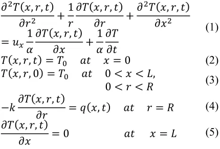
The natural convection and heat diffusion in the axial direction of the tube are assumed to be negligible here. By taking into account the symmetry and neglecting the viscous dissipation, the energy equation governing the problem as well as the proper boundary and initial conditions is given as:
( , , )
+1 ( , , )+ ( , , )
= 1 ( , , )+1
(1)
( , , ) = = 0 (2)
( , , 0) = 0 < < ,
0 < < (3)
− ( , , )= ( , ) = (4)
( , , )
= 0 = (5)
where k and are heat conductivity and diffusivity, respectively.
The fully developed velocity is calculated from:
= 1 − (6)
where U is the mean velocity of the fluid in the tube.
Fig. 1. Tube geometry and coordinates of the
problem adopted.
The unknown heat flux, q(x,t), is discretized into ns spatial components ( ~)
1 m
t
q , q2(tm~), … and qns(tm~), each of which is a function of time. Each spatial component is also assumed to be composed of M discrete time components. All of these components can be gathered in a single vector q:
u0 T0
heat flux q(x,t)
fluid Tf (x,r,t) x
r R R+
⃗ ×
=
( ), ( ), … , ( ), ( ),
( ), … , ( ), … , ( ),
( ), … , ( )
= , , … , , , , … , ; … ;
, , … ,
(7)
The temperature is measured by K sensors, each located at (xk,rk), where k1,2,...,K, and described below:
( , , ) = ( ) = 1,2, … ,
= 1,2, … , (8) The sensitivity coefficients with respect to each component of vector q are defined as:
, , , = , (9)
= , , , = 1,2, … ,= 1,2, … ,
The first derivative appeared in the definition of the sensitivity coefficient can be calculated using finite difference method. Using forward scheme, the sensitivity coefficient is estimated by [3]:
, , , ≅
⎣ ⎢ ⎢
⎡ , , ,
, , … , + , … , −
, , ,
, , … , , … , ⎦
⎥ ⎥ ⎤
(10)
where 105
or 106[3].
The objective function, i.e. the sum of the squared residuals, is defined as:
= (( , , ) −
, , , ⃗) (11)
where Y is the measured temperature and T is the estimated temperature obtained from the solution of the direct forced convection problem (Eqs. (1) - (5)) at the sensor location using estimated heat flux. The objective function is an
implicit function of the unknown heat flux. Vector q should be obtained in such a way that could minimize the objective function.
3. Variable metric method
The aim is to minimize the objective function defined by Eq. (10). The minimization of the objective function, f , which is a function of the unknown heat flux, q, is possible through an iterative method. Searching for the unknown boundary quantity can be proceeded using either direct or descent techniques. Both techniques start with an initial trial solution, q, and then proceed toward the minimum point in a sequential manner. The direct search techniques require only the objective function values and do not use the partial derivatives of the function in finding its minimum. The descent techniques require not only the function evaluations, but also its first and possibly higher order derivatives; therefore, they are also known as gradient based methods. The variable metric method belongs to the gradient based class of the methods and proceeds toward the minimum point by utilizing the following relation:
⃗ = ⃗ + ∗ ⃗ (12)
where * is the search step size, S is the direction of the descent, and i is the iteration number. The direction of the descent is calculated by [13]:
⃗ = − ∇⃗ (13)
The gradient of the objective function in the variable metric method is defined as:
∇⃗ × = (14)
, , … , , , , … , , …
coefficients described in Eq. (10), the gradient
f
can be writhen as:
∇⃗ = −2 × (15)
⎣ ⎢ ⎢ ⎢ ⎢ ⎢ ⎢ ⎢ ⎢ ⎢ ⎢ ⎢ ⎢ ⎢ ⎢ ⎢ ⎢ ⎢ ⎢
⎡ [ ( ) − ( , ⃗)] ( , )
[ ( ) − ( , ⃗)] ( , )
⋮
[ ( ) − ( , ⃗)] ( , )
[ ( ) − ( , ⃗)] ( , )
[ ( ) − ( , ⃗)] ( , )
⋮
[ ( ) − ( , ⃗)] ( , )
⎦ ⎥ ⎥ ⎥ ⎥ ⎥ ⎥ ⎥ ⎥ ⎥ ⎥ ⎥ ⎥ ⎥ ⎥ ⎥ ⎥ ⎥ ⎥ ⎤
The optimal step size *i in the direction of Si is a value of i minimizing f(qiS) with respect to i, i.e., i is the root of the following equation [3]:
⃗ + ⃗
= 0 (16)
By solving Eq. (16), the optimized search step size, *
i
, is obtained as:
∗= (17)
∑ ∑ [ ( ) − ( , ⃗ )]
∑ ∑ ,
∑ ∑ ∑ ∑ ,
In Eq. (13), H is an nn symmetric matrix, which will be modified in each iteration. Depending on which version of variable metric method is chosen, the modification procedure is different. BFGS, DFP, SR1, and Biggs are
various versions of the variable metric method. The modification scheme in each version will be described later in this section.
The variable,
Q
i, for each version of the variable metric method is defined as:= ∇⃗ ( ⃗ ) − ∇⃗ ( ⃗ ) (18)
DFP version modifies the matrix, H , in the following way [13]:
= + ∗
− ( ) ( )
(19)
BFGS is a modified version of DFP and modifies the matrix, H , as follows [5]:
= + ∗
− ( ) ( )
+
(20)
where:
= −
(21)
SR1 version carries out the modification of the matrix, H , in the following manner [5]:
=
+ 1 − ∗ 1∗
× ( ∗ − ) ( ∗ − )
(22)
The Biggs version is designed to modify the matrix, H , in the following way [14]:
= – +
+ 1 + ∗ ∗
(23)
= −2 + ∗ 6
( ⃗ ) − ( ⃗ ) + ∗ ∇⃗ ( ⃗ )
(24)
The DFP and BFGS versions are more widely used than others. The iterative procedure of the variable metric method can be expressed as follows:
1. Suppose an initial guess for q1
and H1. An
identity matrix, I , is usually taken. Set the iteration number i0.
2. Obtain the sensitivity coefficients, )
, , ,
(xk rk tm qm~~n
X , for each component of the vector, q, using Eq. (10).
3. Solve the direct problem based on the guessed q in order to obtain T(xk,rk,tm,qnm~~) using finite volume method.
4. Check the stopping criteria f . Continue if not satisfied.
5. Calculate the gradient of the objective function, fi, using Eq. (15) and obtain the direction of descent from the relation
i i
i H f
S .
6. Normalize Si from:
i i i
S S
S
7. Obtain the optimized search step size using Eq. (17).
8. Compute the new estimate from i
i i
i q S
q1 *
9. Regarding the version of the selected variable metric method, modify the matrix, H using proper relations defined in Eqs. (19) - (24). 10. Set ii1 and return to step 3. 4. Results and discussion
4. 1. Simulated measurements
In this study, the simulated measured data are used in order to evaluate the accuracy of the estimation of the heat flux by variable metric method. To do so, the unknown heat flux,
) , (x t
q , is supposed to vary in the form of step and sine functions.
The time-varying step function is as:
( ) = 50050 33 < ≤ 77 0 < ≤ 33 50 77 < ≤ 110
(25)
and the space-time dependent sine function is defined as:
( , ) = 100 + 150 sin
0.22 (26)
In addition, it is assumed that the fluid in Fig. 1 with the velocity and temperature of 0.2(m s)
and 20C, respectively, flows in a tube with radii R=0.2 (m) and L=0.7 (m). The thermo-physical properties of air at the given temperature are as follows:
= 2.2 × 10 (m s⁄ ) = 0.0262 (W m K⁄ )
In the current study, the final time is set equal to tf 110(s) and the time step of 5(s) is found sufficient for the demanded precision. The sensors in most practical cases are located within the inner wall of the tube.
The measured temperatures used in this study are all simulated. Solving the direct problem using the supposed functions for the unknown heat flux (Eqs. (25) - (26)) will give the simulated temperatures at sensor locations, denoted as Yexa(ti). Since all the actual
measurements are associated with errors, some random errors should be added to the simulated temperatures. Generally, measurements containing random errors denoted as Y(ti) are
simulated by adding an error term to Yexa(ti) as
[3]:
= + (27)
4. 2. Error analysis
It should be noted that the stability of the inverse problem solution can be examined for various levels of measurement errors by generating measurements with different standard deviations . In order to examine the accuracy of the estimation, we define root mean square (RMS) error as:
= ‖ – .‖
‖ ‖ =
1
∑ , − ,
1
∑ ,
× 100
(28)
where the subscript est refers to the estimated heat flux and M is the number of the transient measurements.
4. 3. Step heat flux estimation
The step or pulse heat flux function (Eq. (25)) is applied to evaluate the ability of the inverse method in estimating thermal shocks. Suddenly, the heat flux becomes 10 times greater for a 40-second interval and, then, approaches to its previous value in a moment. The initial guess is equal to zero and the stopping criterion is
considered 6
10
f . The unknown heat flux vector has 21 components.
As the results obtained from different versions of the variable metric method are rather similar to each other, only the estimations obtained using DFP version are illustrated in Fig. 2. As can be observed, the variable metric method has good accuracy in the estimation of the step heat flux, especially around the discontinuity points. The majority of the whole domain inverse methods show instability in the estimation of the unknown step functions [3]. We note that functions containing discontinuities and sharp corners (i.e. discontinuities on their first derivatives) are the most difficult to be recovered by an inverse analysis.
Fig. 2. Estimation of the step heat flux using DFP version for 0.
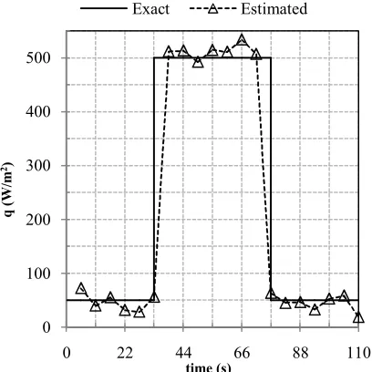
The results obtained from using random measurements with standard deviation of errors of 0.01Tmax are shown in Fig. 3. The estimated
heat flux effectively covers the exact values. It also properly follows the abrupt variation in the heat flux. Similar to other whole domain methods, the solution shows instabilities at the beginning and end of the domain. As shown in Fig. 3, these instabilities are not significant.
Fig. 3. Estimation of the step heat flux using DFP version for 0.01Tmax.
1 101 201 301 401 501
0 22 44 66 88 110
q
(W
/m
2)
time (s)
Exact Estimated
0 100 200 300 400 500
0 22 44 66 88 110
q
(W
/m
2)
time (s)
The convergence details of the solution by different versions of the variable metric method for predicting the step heat flux are shown in Table 1. The results are obtained using random measurements with 0.01Tmax. As shown in
Table 1, SR1 version has the highest convergence speed and lowest error in the estimation of thermal shock and Biggs version is the slowest among the techniques presented here. BFGS, DFP, and Biggs versions estimate the unknown heat flux with the same amount of error. As suggested by Table 1, all the versions estimate the step heat flux with acceptable margin of error.
Table 1. Convergence history of four versions of the variable metric method for estimating the step heat
flux with 0.01Tmax.
Versions No. of
iterations
Convergence time (s)
Error percentage,
eRMS (%)
DFP 7 6 6.4
BFGS 7 5.7 6.4
SR1 7 4.7 5.2
Biggs 7 8 6.4
4. 4. Sine Heat Flux Estimation
The number of unknown vectors for space-time dependent sine heat flux function presented in Eq. (26) is 1071. This number of unknowns makes the current inverse problem so large and difficult. Figure 4 shows the estimated heat flux obtained from the Biggs version at times t= 22.5, 55, 82.5, and 110 (s). The results are presented for errorless simulated measurements, i.e. 0. Due to the similarity between the results of four versions of the variable metric method, only the predicted values obtained by Biggs version are shown in Fig. 4.
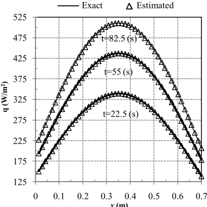
The results obtained from using random measurements with standard deviation of errors of 0.01Tmax are shown in Fig. 5. As is evident in
Fig. 5, the estimated results are in good agreement with the exact values, especially around the final time. In addition, the instabilities in the solution decrease as time increases, which is the same characteristic of all whole domain methods [2].
Fig. 4. Estimating the space-time dependent sine heat flux using Biggs version for 0.
Fig. 5. Estimating the space-time dependent sine heat flux using Biggs version for 0.01Tmax.
The convergence details of the solution using different versions of variable metric method for predicting sine heat flux with 0.01Tmax are shown in Table 2. All the four versions have approximately the same error bound. SR1 version converges more rapidly and its calculation cost is the lowest among other versions. On the other hand, Biggs version is the slowest and imposes the most calculation cost on the inverse solution. The trends shown
125 175 225 275 325 375 425 475 525
0 0.1 0.2 0.3 0.4 0.5 0.6 0.7
q
(W
/m
2)
x (m)
t=82.5 (s)
t=55 (s)
t=22.5 (s)
Exact Estimated
50 150 250 350 450 550
0 0.1 0.2 0.3 0.4 0.5 0.6 0.7
q
(W
/m
2)
x (m)
t=82.5 (s)
t=55 (s)
t=22.5 (s)
in Table 2 for sine function are similar to those obtained for a step function in Table 1.
Table 2. Convergence history of four versions of variable metric method for estimating sine heat flux with 0.01Tmax
.
V
er
si
on
s
N
o.
o
f
it
er
at
ions
C
onve
rge
n
ce
ti
m
e
(s
)
Error percentage,eRMS (%)
t
=
22
.5
(
s
)
t
=
55
(
s
)
t
=
82
.5
(
s
)
t
=
110
(
s
)
DFP 7 6 7.9 5 4.8 2.8
BFGS 7 5.7 7.2 6.6 4.7 2.3
SR1 7 4.7 7.2 6.6 4.7 2.3
Biggs 7 8 7.2 6.6 4.7 2.3
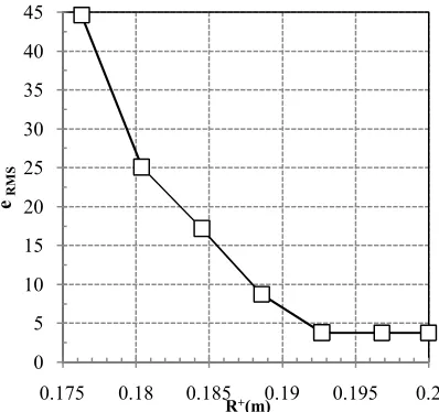
4. 5. Effect of sensor location
The effect of changing the sensor location on accuracy of the DFP version in estimating the step heat flux is presented in Fig. 6. The variation of root mean square error with the distance between the sensor location and tube axis is shown in Fig. 6. The accuracy of the solution increases with increasing the distance between the sensor location and the tube axis. It can be concluded from Fig. 6 that locating the sensor as close as possible to the unknown boundary condition, i.e. the wall heat flux, will increase the accuracy of the solution.
5. Conclusions
The variable metric method was applied to estimate the unknown space-time dependent heat flux imposed to the outer wall of a tube with forced convection inside it. The simulated temperature measurements at certain points within the flow field were input to the analysis. The accuracy of the method in estimating an unknown step heat flux and a space-time dependent sine function was examined and the results obtained by four different versions of the presented method were compared with each other. Furthermore, the effect of the sensor installation location on the accuracy of the solution was evaluated. Numerical results
indicated that the variable metric method estimated the unknown heat flux with acceptable accuracy even when the temperature measurements with error were used. Comparison of all four versions showed that the SR1 version was the most effective method with minimum convergence time and maximum accuracy. On the other hand, the BIGS method was found to be the slowest one in converging to the final solution with slightly larger error than other methods.
Fig. 6. Variation of the solution error with the distance between the sensor location and tube axis in estimating the step heat flux using DFP version for
0
.
Acknowledgments
The authors wish to thank Dr. Kamran Alba, Assistant Professor of Engineering Technology Department of University of Houston, for his invaluable comments on grammar, organization and the theme of the manuscript.
References
[1]
J. C. Bokar, and M. N. Ozisik, “An inverse analysis for estimation of time-varying inlet temperature in laminar flow inside a parallel plate duct”, International0 5 10 15 20 25 30 35 40 45
0.175 0.18 0.185 0.19 0.195 0.2
eR
M
S
Journal of Heat and Mass Transfer, Vol. 38, No. 1, pp. 39-45, (1995).
[2]
J. V. Beck, and K. A. Woodbury, “Inverse problems and parameter estimation: integration of measurements and analysis”, Measurement Science and Technology, Vol. 9, No. 6, pp. 839-847, (1998).[3]
M. N. Ozisik, and H. R. B. Orlande,Inverse Heat Transfer: Fundamentals and Applications, 1st ed., Taylor & Francis, New York, (2000).
[4]
O. M. Alifanov, Inverse Heat TransferProblems, 1st ed., Springer-Verlag,
Berlin, (1994).
[5]
L. Luksan, and E. Spedicato, “Variable metric methods for unconstrained optimization and nonlinear least squares”, Journal of Computational and Applied Mathematics, Vol. 124, No. 1-2, pp. 61-95, (2000).[6]
C. H. Huang, and M. N. Ozisik, “Inverse problem of determining unknown wall heat flux in laminar flow through a parallel plate duct”, Numerical Heat Transfer, Part A: Applications: An International Journal of Computation and Methodology, Vol. 21, No. 1, pp. 55-70, (1992).[7]
M. J. Colaco, and H. R. B. Orlande, “Inverse forced convection problem of simultaneous estimation of two boundary heat flux in irregularly shaped channels”,Numerical Heat Transfer, Part A: Applications, Vol. 39, No. 7, pp. 737- 760, (2001).
[8]
P. Ding, and W. Q. Tao, “Estimation of unknown boundary heat flux in laminar circular pipe flow using functional optimization approach: effects ofReynolds numbers,” Journal of Heat Transfer, Vol. 131, No. 2, pp. 1-9, (2009).
[9]
C. H. Huang, I. C. Yuan, and H. Ay, “A three-dimensional inverse problem in imaging the local heat transfer coefficients for plate finned-tube heat exchangers”, International Journal of Heat and Mass Transfer, Vol. 46, No. 19, pp. 3629-3638, (2003).[10]
W. L. Chen, and Y. C. Yang, “An inverse problem in determining the heat transfer rate around two in line cylinders placed in a cross stream”, Energy Conversion and Management, Vol. 48, No. 7, pp. 1996-2005, (2007).[11]
F. Bozzoli, L. Cattani, C. Corradi, M. Mordacci, and S. Rainieri, “Inverse estimation of the local heat transfer coefficient in curved tubes: a numerical validation”, Journal of Physics:Conference Series, Vol. 501, No.
012002, (2014).