http://www.sciencepublishinggroup.com/j/ajtas doi: 10.11648/j.ajtas.20170605.13
ISSN: 2326-8999 (Print); ISSN: 2326-9006 (Online)
Using the Second Order Kronecker Model in
Simplex–Centroid Design in Formulating Optimum Dairy
Feed
Robert Muriungi Gitunga
1, 2, *, Joseph Kipsigei Koske
2, Johnstonne Mutiso Muindi
2 1Department of Mathematics, Meru University of Science and Technology, Meru, Kenya2
Department of Statistics and Computer Science, Moi University, Eldoret, Kenya
Email address:
*
Corresponding author
To cite this article:
Robert Muriungi Gitunga, Joseph Kipsigei Koske, Johnstonne Mutiso Muindi. Using the Second Order Kronecker Model in Simplex– Centroid Design in Formulating Optimum Dairy Feed. American Journal of Theoretical and Applied Statistics.
Vol. 6, No. 5, 2017, pp. 236-247. doi: 10.11648/j.ajtas.20170605.13
Received: March 18, 2017; Accepted: April 8, 2017; Published: September 8, 2017
Abstract:
The Second order kronecker model for simplex-centroid design was fitted where data was for feed supplements blend using a mixture of soya beans, maize jam, cotton seed and fish meal guided by design points in the simplex-centroid design and the respose was the yield of milk in litres. The main objective was to fit a Kronecker model in the simplex-centroid design to formulate optimum dairy meal concentrates. Use the data to fit the second order kronecker model for four components simplex-centroid design. From the Kronecker regression function, coefficient matrix was derived from selected parameter subsystem of interest, moment matrix was then obtained. Information matrix and improved information matrix were derived. The collected data was fitted in the derived Kronecker model and the estimates of the parameters as well as overall model performance were numerically obtained. ANOVA was run to incorporate the constant term. From the analysis it was found that Kronecker model provided a good fit. Therefore the results support that the feed supplement had significant effect to milk productivity. For optimal production the research recommend that more than one ingredients need to be blend. Blends with soya beans and fish meal in two, three and four ingredients were statistically significant and therefore recommended for optimal milk production. From the ANOVA it was found that other factors not included in this study affect milk productivity and therefore the research recommends further studies be done to investigate those other factors such as the breeds, feeding practices and also effect of supplement to other dairy products.Keywords: Kronecker Model, Simplex-Centroid, Coefficient Matrix, Information Matrix
1. Introduction
In this section we discussed the background of the study by describing the mixture experiment, dairy meal concentrates and their importance to dairy animals and their formulation. Scholarly studies are reviewed here. We then formulate the study problem giving the study objectives. The scope of the study is also discussed incorporating the study assumptions.
Background of the study
Mixture experiment involves proportion of one or more ingredients for optimizing one or more criteria. There are often many competing criteria that could be considered in
selecting the design, and one is typically forced to make trade-offs between these objectives when choosing competing design. The measured response is assumed to depend only on the proportions of the ingredients present in the mixture and not on the amount of the mixture, [1].
groups). It is common to show the energy and protein contents of the diet but comprehensive information on concentrations of mineral elements and amino acids may also be provided. The balancing of animal feeds are based on the principles of feed formulation.
The objective of feed formulation is to utilize knowledge about nutrients, feedstuffs and animals in the development of nutritionally adequate rations that will be eaten in sufficient amounts to provide the desired level of production at reasonable cost. To achieve this objective, a blend of knowledge is required for optimum results. A ration is balanced when all the required nutrients are present in the feed ingested by the animal during a period of 24 hours.
Dairy animal’s daily nutrient requirements should be calculated on realistic production goals. Specific factors to consider are milk production and composition, animal activity, body weight, stage of pregnancy and changes in body condition. In practice, it may be necessary to consider only those nutrients that are likely to be limiting or deficient (energy, proteins, macro-elements and amino acids).
Present day high milk producing animals in the Eastern Africa region are the result of years of genetic improvement programmes. However, poor feed, inadequate in both quality and quantity, is a major constraint in efforts to improve the productivity of livestock in many smallholder production systems in the region; whether mixed farming, pastoral or agro-pastoral. The principal sources of feed for ruminants in mixed crop-livestock systems are crop residues complemented with forage collected from communal land, forests, roadsides or fallow land, or by grazing animals on those lands. This feeding regime often does not meet the nutritional requirements for maintaining high milk production of dairy animals. Adding a supplement of concentrates helps meet the high demand for nutrients needed to sustain high milk production.
In Kenya, milk is traditionally produced at the lowest possible cost from a pastures and crop residues-based feeding system. The price of milk has been low and constantly fluctuates with seasons. Since mid-2002 milk market prices in Kenya have been rising steadily, and there has been a tendency to move from pastoral milk production to more intensive systems, where commercial dairy concentrates are fed as supplements. Such a scenario calls for more localized feeding methods such as Total Mixed Ration (TMR) or supplementations based on simple feed formulation approaches.
Various evaluation techniques have been used in the formulation of dairy feeds. Wagner and Stanton in [2], used Pearson square. However this technique can only balance one nutrient at a time. Least cost formulation based on linear programming has also been used, [3]. This technique requires commercial feed software which is costly for most extension organization in developing countries and return on investment when using them on a small scale does not justify its purchase.
This research is an extension of Muriungi, et al. in [4], where polynomial model in simplex-Centroid for four
components design to formulate optimum dairy feed was used. We therefore adopts a mixture experiment design which is a special type of a response surface experiment in which the factors are the ingredients or components of the mixture; the response is a function of the proportions of each ingredient. The proportional amounts of each ingredient are typically measured by weight, volume, and ratio and so on as described by Myers, et-al in [5]. They also defined Response surface methodology as a collection of statistical and mathematical techniques useful for developing, improving and optimizing process, and response is the performance measure of a given process. However, we fitted the second order Kronecker model for the four components in simplex-centroid design.
The objective of the study was to use the second order Kronecker model for four components in Simplex-Centroid design to formulate the optimum dairy concentrate. We therefore seek to derive the second order Kronecker model using a subsystem of interest and fit data on the model to determine the points of the design that yields optimum response.
Dean, et al. in [6], used least- cost feed formulation for dairy cattle to the next logical step of profit maximization. Linear programming model presented selects simultaneously the concentrate and roughage components of the ration, the roughage-concentrate ratio, level of feeding per cow and quantity of milk production maximizing income above feed costs. They presented the nutritional and economic aspects of the model in mathematical form. This was followed by illustrations on nutritional specifications which include body maintenance requirements and milk production response curve associated with alternative levels of energy and protein fed. They recommended an improvement of the model by research designed to define more precisely the milk production response relationships for cows of different ability, size, breed, stage of lactation and other determinants.
Chakeredza et al. in [7], used linear programming to formulate a least cost ration. The least cost formulation was described as a mathematical solution based on linear programming.
Mahmut, et al. in [8], used Mixture design to investigate the effects of four different gums (xanthan gum, guar gum, alginate and locust bean gum) and their combinations on the rheological properties of a prebiotic model instant hot chocolate beverage (including 3.5% inulin) and to determine their interactions in the model beverage. Simplex centroid mixture design was applied to predict the physicochemical (soluble solids, pH, colour properties) and rheological parameters (consistency index (K), flow behaviour index (n) and apparent viscosity (η50)) of the samples. In the model, the optimum gum combination was found by simplex centroid mixture design as 59% xanthan gum and 41% locust bean gum, and the highest K value was 33.56 Pa sn. The increase of guar gum and alginate in the gum mixture caused a decrease in the K value of the sample.
cocoyam flours. Ten formulations were obtained from this design.
In their paper “A V-optimal design for Scheffe’ polynomial model”, Shuangzhe and Heinz in [10], applied the weighted simplex centroid design to obtain V-optimal allocations of the observations and showed optimality over the entire simplex using the equivalence theorem.
Koske et-al. in [11], indicated that the goal of an experimenter is to obtain a design that gives maximum information. They investigated mixture experiments on second degree Kronecker model. They showed how a design can be improved by using a parameter subspace.
Gaylor and Sweeny in [12] studied optimum allocation. They said that a region of interest does not necessarily correspond to the region available for experimentation 0≤ ≤x 1. They said that the allocation of experimental data points minimizes the average variance of the predicted values occurring according to the density function in the region of prediction is derived as ŷ=α+βz. The errors of this relation were assumed to be uncorrelated and of a common variance
2
y
σ
.Coetzer and Focke in [13], used mixture design in mixing fluids. They viewed mixture conceptually as a hypothetical collection of fluid clusters. The mixture model was defined by prescription for estimating fluid cluster properties and combining them to yield an overall mixture property. A particular flexible form was obtained using a generalized weighted power- means with the weighting based on global mole fractions xi, 0≤ ≥xi 1,
∑
xi=1,i=1, 2⋯q . Optimaldesigns for estimating the parameters in the generalized weighted power-mean mixtures were presented. They concluded that the simplex centroid design is very efficient in estimating the parameters of the model and that it is not dependent on initial guesses for the parameter estimates. They suggested that these designs may be employed for determining initial parameter estimates for employing a sequential design strategy.
Scope of the study
Second degree Kronecker model for four mixture components was derived and data fitted on the model. This was numerically analyzed.
The second-degree Kronecker model has all entries homogeneous in degree four and reflects the statistical properties of a design
The primary concern of the experimenter was to learn more about the subsystems of interest. Therefore the coefficient matrix K was computed from given subsystems of interest. This allows the designer to evaluate the performance of a design relative to the subsystems of interest only.
From the coefficient matrix, moment matrix was derived and the information matrix derived.
Data was fitted on the Kronecker model and the model was analyzed.
The study assumed that there was homogeneity in data primary feeding practices for the dairy animals in which the data was collected as well as control of external factors such
as diseases.
2. Materials and Methods
2.1. Introduction
In this section we discuss the general design problem for the kronecker model, data collection and analysis procedure were also be discussed.
2.2. Kronecker Model
The study was extended to designing a problem that will help in obtaining a design with maximum information for the maximal parameter subsystem Kθ′ , subject to the side’s conditions. Kronecker regression model was appropriate for this purpose. In this study we fitted the second order Kronecker model for the four ingredients.
The mixture ingredients t1, t2 … tm are such that ti≥0
such that
∑
ti=1Thus the experimental region was given bythe probability simplex
1 1
1 { ( ,..., ) ' [0,1] 1},
m
m m
i
t
t
t
t
whereT
ε=
= =
∑
= tm
t T
∈
(1)For this study, m=4
The second order Kronecker regression model for four ingredients was used to model the expected response ( )E Yt
as was suggested by Draper and Pukelsheim in [14]
1 1
[ ] ( ) '
m m t i j ij
i j
t t
t t
Y
θ
θ= =
Ε =
∑∑
= ⊗ (2)The second degree Kronecker model was given by
( )
( )
2(
)
, 1 ,
'
m
t ii i ij ji i j i j i j
E Y f t θ θ t θ θ t t
=
= =
∑
+∑
+ (3)WhereYt the observed response under the experimental conditions t∈T was taken to be a scalar random variable and
(
)
211, 22,..., '
m mm R
θ θ θ
Θ = ∈ (4)
unknown parameter.
The moment matrix was determined by
( )
( ) ( )
'T
M τ =
∫
f t f t dτ (5)With the unknown parameter vector
11 12
( , ,..., mm )
θ= θ θ θ εℜΜ and the regression function,
( )
f t = ⊗t t for all ti (observations) from an experiment are assumed to be of equal unknown variance and are uncorrelated.
2 2
1
11 12 1 2 13 1 3 14 1 4 21 2 1 22 2 23 2 3 24 2 4
2 2
31 3 1 32 3 2 33 3 34 3 4 41 4 1 42 4 2 43 4 3 44 4
( )
E y t
t t
t t
t t
t t
t
t t
t t
t t
t t
t
t t
t t
t t
t t
t
θ θ
θ
θ
θ
θ
θ
θ
θ
θ
θ
θ
θ
θ
θ
θ
= + + + + + + + +
+ + + + + + +
(6)
We derived the coefficient, moment and the information matrices in order to obtain an optimal response in terms of mixture components
2.2.1. Coefficient Matrix (K )
Sometimes it is not necessary to work with the full parameter system θ, and therefore we may wish to study s
out of the k, s≤k components. This is achieved by studying the linear parameter subsystem of interest K'θ for some
k×s matrix K. K is referred to as the coefficient matrix of the parameter subsystem K'θ.
Draper and Pukelshein in [15], proposed a model representation involving the Kronecker square t⊗t , the
2
1
m × vector consisting of the squares and cross products of the components of t in lexicographic order.
Given the regression function, we obtained the order as;
( )
2 211 1 12 1 2 13 1 3 14 1 4 21 2 1 22 2 23 2 3 24 2 4 31 3 1 32 3 2
2 2
33 3 34 3 4 41 4 1 42 4 2 43 4 3 44 4
f t t t t t t t t t t t t t t t t t t t
t t t t t t t t t t
θ θ θ θ θ θ θ θ θ θ
θ θ θ θ θ θ
= + + + + + + + + + +
+ + + + + (7)
In this research we used a subsystem of interest given by the equation.
'
K θ=
11 12 21 13 31 14 41
22 23 32 24 42
33 34 43
44
2
2
2
2
2
2
θ
θ θ
θ θ
θ θ
θ
θ θ
θ θ
θ
θ θ
θ
+
+
+
+
+
+
(8)
Where θ is the vector of the full parameters and the vector on the right hand side represent the subsystems of interest. This equation was used to determine the coefficient matrix K.
From the subsystems of interest vector, the full Kronecker regression model was reduced to the following model
( )
(
)
(
)
(
)
(
)
(
)
(
)
2 2
11 1 12 21 12 21 13 31 13 31 14 41 14 41 22 2
2 2
23 32 23 32 24 42 24 42 33 3 34 43 34 43 44 4
1 1 1
2 2 2
1 1 1
2 2 2
E y t t t t t t t t
t t t t t t t t
θ θ θ θ θ θ θ θ
θ θ θ θ θ θ θ θ
= + + + + + + + + + + +
+ + + + + + + + + +
(9)
2.2.2. Moment Matrix (M)
From the General Equivalence Theorem, if M∈ ℳ is a competing moment matrix that is feasible for K'θ with information matrix ( )
K
C=
C
M , Then M isϕ
− optimal for'
K θ in
ℳ
if and only if there exists a NND(s) matrix D, that solves the polarity equation( )C α( )D traceCD 1
ϕ
ϕ
− = = (10)And also there exists a generalized inverse G of M, such that the matrix N=GKCDCK G' ' that satisfies the normality inequality
But for optimality, equality is obtained in the normality inequality if M is inserted instead of A.
For the simplex shaped experimental region, the moment matrix was given by
( )
( ) ( )
't
M η =
∫
f t f t dt (12)This equation was adapted in our research since we used a model of subsystem of interest rather than the full regression range.
From the four components simplex-centroid design we had the 4 designs η η η1, 2, 3andη4 for the pure, binary, ternary and the overall centroid. We therefore derived the moment matrix by summing the individual design moment matrix
( )
( )
1( )
2( )
3( )
44 6 4 1
15 15 15 15
M n = M η + M η + M η + M η (13)
These design moments were derived as follows where R-software was used to derive the numerical values.
Using the Kronecker product, the four factors, (t1, t2, t3, t4)=(1, 0, 0, 0), (0, 1, 0, 0), (0, 0, 1, 0) and (0, 0, 0, 1), for the pure mixture blends were obtained as ⨂ ⨂ ′; resulting in matrices for each of the design point. This procedure was repeated for the four design points namely, pure, binary, tertiary and the centroid.
In the Kronecker model,
τ
has moment matrix( )τ τ(t t t)( t) τ
Μ =∫ ⊗ ⊗ ∂ (14)
The set of moments of order four determines all lower order moments. For instance the pure third moment expands to order four by way of
( )
3
3
t
1 t1 t2 d 4 31µ =
∫
+ τ= +
µ µ
(15)Other lower moments were derived as follow
( )
2
21
t
1t2 t1 t2 d 31 22µ =
∫
+ τ=
µ
+
µ
(16)( )
2
2
t
1 t1 t2 d 3 21µ =
∫
+ τ= +
µ µ
(17)=
(
µ4+µ31) (
+ µ31+µ22)
(18) =µ4+2µ31+µ22 (19)( )
11 t t1 2 t1 t2 d 21 21
2
21µ =
∫
+ τ=
µ
+
µ
=
µ (20)=2
(
µ31+µ22)
(21) =2µ31+2µ22 (22)2.2.3. Information Matrix
Pukelsheim in [16], gave the definition of an information matrix as: For a design
ξ
with the moment matrix M, theinformation matrix for K'θwith KxS coefficient matrix K of full column S, is defined to be CK(Μ) where the mapping
K
C from the cone NND (K) into the space sym(S) is given by
( )
;'
min
S K S
k
L R LK I
C A LAL
×
∈ =
= For all
A
∈
NND K
( )
(23)Where the minimum is taken according to Loewner ordering over all the left inverses L of K
In our design, given that the coefficient matrix has been determined from the subsystem of interest and the moment matrix has been derived, then the coefficient matrix C was given by
',
C=LML (24)
Where L is the left inverse of K given by;
1 '
( 'K)
L= K − K (25)
2.3. Data Collection and Analysis
In this research, the researcher used secondly data collected in Muriungi et al in [4] to fit the Kroneckor model.
The collected data was fitted in the Kronecker model. The coefficient of the model was derived using the least square equation
(
)
1' '
X X X Y
β = − (26)
To carry ANOVA test in order to determine the significance of each design in the model and to evaluate the overall fitness of the model, we first calculated the F-statistics using the equation;
(
)
(
)
/ 1
/
SSR p F
SSE N p − =
− (27)
Where N is the total observations in this case N=75 and P the number of design points.
2 75
1
N u u
SSE y y
= ∧ −
=
= −
∑
(28)2 75
1
N u u
SSR y y
= ∧
=
= −
∑
(29)u
y is the value of the uth observation
u
y
∧
is the predicted value of the response corresponding to the uth observation which is determined from the model by substituting the parameter estimates
y
−
We therefore determine the adjusted coefficient of determination RA2 utilizing the equation
2 1 / ( )
/ ( 1)
A
SSE N p
R
SST N
− = −
− (30)
Where SST =SSR+SSE (31)
3. Results
3.1. Introduction
From the full parameter system Kronecker regression function in (26), we derived a model that uses the selected subsystem of interest as described in section 3.2. In the
succeeding section we used the model of subsystem of interest parameters to determine the coefficient matrix.
3.2. Kronecker Model
From the full parameter system Kronecker regression function in (6), we derived a model that uses the selected subsystem of interest as described in section 3.2.1 In the succeeding section we used the model of subsystem of interest parameters to determine the coefficient matrix.
3.2.1. Coefficient Matrix
Using (8), we determined the Transpose of the coefficient matrix as.
K’ =
1 0 0 0 0 0 0 0 0 0 0 0 0 0 0 0
0 0.5 0 0 0.5 0 0 0 0 0 0 0 0 0 0 0
0 0 0.5 0 0 0 0 0 0.5 0 0 0 0 0 0 0
0 0 0 0.5 0 0 0 0 0 0 0 0 0.5 0 0 0
0 0 0 0 0 1 0 0 0 0 0 0 0 0 0 0
0 0 0 0 0 0 0.5 0 0 0.5 0 0 0 0 0 0
0 0 0 0 0 0 0 0.5 0 0 0 0 0 0.5 0 0
0 0 0 0 0 0 0 0 0 0 1 0 0 0 0 0
0 0 0 0 0 0 0 0 0 0 0 0.5 0 0 0.5 0
0 0 0 0 0 0 0 0 0 0 0 0 0 0 0 1
(32)
3.2.2. Moment Matrix
For the four components vector
(
t t t t1, , ,2 3 4)
/, we utilize the kronecker product to obtain the moment matrix( )
M τ =
/
1 1 1 1
2 2 2 2
3 3 3 3
4 4 4 4
t t t t
t t t t
t t t t
t t t t
⊗ × ⊗
(33)
This will yield a 16 by 16 matrix.
From section 2.1.2, we noted that the set of moments of order four determines all the lower order moments. For the four-ingredient model, given an arbitrary exchangeable design
τ
, the fourth order moments are4 4 t d1
µ =
∫
τ− (34)3 31 t t d1 2
µ =
∫
τ− (35)2 2 2
211 t t t d1 2 3 , 22 t t d1 2 , 1111 t t t t d1 2 3 4
µ =
∫
τ µ− =∫
τ µ− =∫
(36)4 31 31 31 31 22 211 211 31 211 22 211 31 211 211 22 31 22 211 211 22 31 211 211 211 211 211 1111 211 211 1111 211 31 211 22 211 211 211 211 1111 22 211 31 211 211 1111 211 211 31 211 211 22 211 211
µ µ µ µ µ µ µ µ µ µ µ µ µ µ µ µ
µ µ µ µ µ µ µ µ µ µ µ µ µ µ µ µ
µ µ µ µ µ µ µ µ µ µ µ µ µ µ µ µ
µ µ µ µ µ µ µ1111 211 211 1111 211 211 22 211 211 31
31 22 211 211 22 31 211 211 211 211 211 1111 211 211 1111 211
22 31 211 211 31 4 31 31 211 31 22 211 211 31 211 22
211 31 211 1111 211 31 22 211 211 22 31 211 1
µ µ µ µ µ µ µ µ µ
µ µ µ µ µ µ µ µ µ µ µ µ µ µ µ µ
µ µ µ µ µ µ µ µ µ µ µ µ µ µ µ µ
µ µ µ µ µ µ µ µ µ µ µ µ µ111 211 211 211
211 211 1111 211 211 31 211 22 1111 211 211 211 211 22 211 31 31 211 22 211 211 211 211 1111 22 211 31 211 211 1111 211 211 211 211 211 1111 211 31 22 211 211 22 31 211 1111 211 211 21
µ µ µ
µ µ µ µ µ µ µ µ µ µ µ µ µ µ µ µ
µ µ µ µ µ µ µ µ µ µ µ µ µ µ µ µ
µ µ µ µ µ µ µ µ µ µ µ µ µ µ µ µ 1
22 211 31 211 211 22 31 211 31 31 4 31 211 211 31 22
211 1111 211 211 1111 211 211 211 211 211 31 22 211 211 22 31 31 211 211 22 211 211 1111 211 211 1111 211 211 22 211 211 31 211 211 1111 211 211
µ µ µ µ µ µ µ µ µ µ µ µ µ µ µ µ
µ µ µ µ µ µ µ µ µ µ µ µ µ µ µ µ
µ µ µ µ µ µ µ µ µ µ µ µ µ µ µ µ
µ µ µ µ µ µ31 211 22 1111 211 211 211 211 22 211 31
211 1111 211 211 1111 211 211 211 211 211 31 22 211 211 22 31
22 211 211 31 211 22 211 31 211 211 22 31 31 31 31 4
µ µ µ µ µ µ µ µ µ µ
µ µ µ µ µ µ µ µ µ µ µ µ µ µ µ µ
µ µ µ µ µ µ µ µ µ µ µ µ µ µ µ µ
(37)
In the simplex -centroid design with four components there are 15 design points. Four elementary centroid designs: η1
which is supported on the vertices, η2 on the edge midpoints, η3 on the ternary and η4 on the overall centroid point. This is
given as in the equations below where there are 4 η1design points, 6 η2 design points, 4 η3 design points and 1 η4 design
point. 1 0 0 0 0 1 0 0 0 0 1 0 0 0 0 1 1 2 1 2 0 0 1 2 0 1 2 0 1 2 0 0 1 2 0 1 2 1 2 0 0 1 2 0 1 2 0 0 1 2 1 2 1 3 1 3 1 3 0 1 3 1 3 0 1 3 1 3 0 1 3 1 3 0 1 3 1 3 1 3 1 4 1 4 1 4 1 4 (38)
Therefore the moments of order four of these designs are, respectively found as follows: For µ4 we average all the element to power four of any of the row in the design. i.e
( )
44 4
4
1
... 0.08190
15
1
1
4
d
t
µ τ = = + + = ∫
(39)For µ22, we take any two rows, square the elements, sum the corresponding product of the two rows and average the sum.
i.e
(
)
2 2 22 1 2
1
0.00607 15
2 2
2
2
...
1
1
0
1
4
4
d
t t
µ τ = = =
× +
+
×
∫
(40)For µ31, we take the cube of any row and multiply it with corresponding elements of any other row. These product are
summed and its average determined.
( )
3 1 31 1 2
1
0.00607 15
3 1
1
3
...
1
1
0
1
4
4
d
t t
µ τ = = =
× +
+
×
∫
(41)For µ211, we take the square of the elements in any row and multiply with corresponding elements in any other two rows.
(
)
1 2
211 1 3
1
0.00108 15
2 1 1
1 1 2 1
2
t
d1
0 0
...
1
4
1
4
1
4
t t
µ τ
= = =
× × +
+
×
×
∫
(42)
For µ1111, we sum and average the products of the corresponding elements in the four rows
(
)
1
1 1
1111 1 4
3 1
0.00026 15
2 1 1 1
1 1 1
1 1
2
1
0 0 0
...
1
4
1
4
1
4
1
4
= = =
× × × +
+
×
×
×
∫
d
t
t
t
t
µ τ (43)
The results from (39) to (43) were substituted to (37) to yield the moment matrix M.
However using (38), we numerically obtained the moment matrix M
( )
η . This was done by first obtaining the moment matrix for the designs in the simplex centroid;M( )
η1 , M( )
η2 , M( )
η3 and M( )
η4 .Both method will yield the numerical values of the moment matrix as: Matrix M
0.08190 0.00607 0.00607 0.00607 0.00607 0.00607 0.00108 0.00108 0.00607 0.00108 0.00607 0.00108 0.00607 0.00108 0.00108 0.00607 0.00607 0.00607 0.00108 0.00108 0.00607 0.00607 0.00108 0.00108 0.00108 0.00108 0.00108 0.00026 0.00108 0.00108 0.00026 0.00108 0.00607 0.00108 0.00607 0.00108 0.00108 0.00108 0.00108 0.00026 0.00607 0.00108 0.00607 0.00108 0.00108 0.00026 0.00108 0.00108 0.00607 0.00108 0.00108 0.00607 0.00108 0.00108 0.00026 0.00108 0.00108 0.00026 0.00108 0.00108 0.00607 0.00108 0.00108 0.00607 0.00607 0.00607 0.00108 0.00108 0.00607 0.00607 0.00108 0.00108 0.00108 0.00108 0.00108 0.00026 0.00108 0.00108 0.00026 0.00108 0.00607 0.00607 0.00108 0.00108 0.00607 0.08190 0.00607 0.00607 0.00108 0.00607 0.00607 0.00108 0.00108 0.00607 0.00108 0.00607 0.00108 0.00607 0.00108 0.00026 0.00108 0.00607 0.00607 0.00108 0.00108 0.00607 0.00607 0.00108 0.00026 0.00108 0.00108 0.00108 0.00108 0.00108 0.00026 0.00108 0.00108 0.00607 0.00108 0.00026 0.00607 0.00108 0.00108 0.00108 0.00108 0.00607 0.00108 0.00607 0.00607 0.00108 0.00607 0.00108 0.00108 0.00108 0.00108 0.00026 0.00607 0.00108 0.00607 0.00108 0.00108 0.00026 0.00108 0.00108 0.00108 0.00108 0.00108 0.00026 0.00108 0.0180.7 0.00607 0.00108 0.00108 0.00607 0.00607 0.00108 0.00026 0.00108 0.00108 0.00108 0.00607 0.00108 0.00607 0.00108 0.00108 0.00607 0.00607 0.00108 0.00607 0.00607 0.08190 0.00607 0.00108 0.00108 0.00607 0.00607 0.00108 0.00026 0.00108 0.00108 0.00026 0.00108 0.00108 0.00108 0.00108 0.00108 0.00607 0.00607 0.00108 0.00108 0.00607 0.00607 0.00607 0.00108 0.00108 0.00607 0.00108 0.00108 0.00026 0.00108 0.00108 0.00026 0.00108 0.00108 0.00607 0.00108 0.00108 0.00607 0.00108 0.00108 0.00026 0.00108 0.00108 0.00607 0.00108 0.00607 0.00026 0.00108 0.00108 0.00108 0.00108 0.00607 0.00108 0.00607 0.00108 0.00026 0.00108 0.00108 0.00026 0.00108 0.00108 0.00108 0.00108 0.00108 0.00607 0.00607 0.00108 0.00108 0.00607 0.00607 0.00607 0.00108 0.00108 0.00607 0.00108 0.00607 0.00108 0.00607 0.00108 0.00108 0.00607 0.00607 0.00607 0.00607 0.00607 0.08190
(44)
3.2.3. Information Matrix (C)
Information matrix was determined by utilizing (24) and (25). From (24) and using R- software, the left inverse of the coefficient matrix was derived as;
L=
1 0 0 0 0 0 0 0 0 0 0 0 0 0 0 0
0 1 0 0 1 0 0 0 0 0 0 0 0 0 0 0
0 0 1 0 0 0 0 1 0 0 0 0 0 0 0 0
0 0 0 1 0 0 0 0 0 0 0 0 1 0 0 0
0 0 0 0 0 1 0 0 0 0 0 0 0 0 0 0
0 0 0 0 0 0 1 0 0 1 0 0 0 0 0 0
0 0 0 0 0 0 0 1 0 0 0 0 0 1 0 0
0 0 0 0 0 0 0 0 0 0 1 0 0 0 0 0
0 0 0 0 0 0 0 0 0 0 0 1 0 0 1 0
0 0 0 0 0 0 0 0 0 0 0 0 0 0 0 1
(45)
0.08190 0.01214 0.00715 0.01214 0.00607 0.00216 0.00216 0.00607 0.00216 0.00607 0.01214 0.02428 0.00432 0.00432 0.01214 0.00432 0.00432 0.00216 0.00104 0.00216 0.00715 0.00432 0.00685 0.00432 0.00715 0.00432 0.00685 0.00715 0.00432 0.00715 0.01214 0.00432 0.00432 0.02428 0.00216 0.00104 0.00432 0.00216 0.00432 0.01214 0.00607 0.01214 0.00715 0.00216 0.08190 0.01214 0.01214 0.00607 0.00216 0.00607 0.00216 0.00931 0.00432 0.00104 0.01214 0.02428 0.00432 0.01214 0.00432 0.00216 0.00216 0.00432 0.00685 0.00432 0.01214 0.00432 0.01847 0.00216 0.00432 0.01214 0.00607 0.00216 0.00715 0.00216 0.00607 0.01214 0.00216 0.08190 0.01214 0.00607 0.00216 0.00104 0.00432 0.00432 0.00216 0.00432 0.00432 0.01214 0.02428 0.01214 0.00607 0.00216 0.00715 0.01214 0.00607 0.00216 0.01214 0.00607 0.01214 0.08190
(46)
3.3. Fitting Data in the Kronecker Model for Four Components Simplex-Centroid Design
As indicated in section 1.1 and 2.2, we made use of data collected by Muriungi et.al. in [4] below
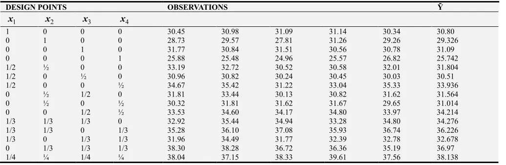
Table 1. Experimental Data on Milk Production in Liters.
DESIGN POINTS OBSERVATIONS Ỹ
1
x x2 x3 x4
1 0 0 0 30.45 30.98 31.09 31.14 30.34 30.80
0 1 0 0 28.73 29.57 27.81 31.26 29.26 29.326
0 0 1 0 31.77 30.84 31.51 30.56 30.78 31.09
0 0 0 1 25.88 25.48 24.96 25.57 26.82 25.742
1/2 ½ 0 0 33.19 32.72 30.52 30.58 32.01 31.804
1/2 0 ½ 0 30.96 30.82 30.24 30.45 30.03 30.51
1/2 0 0 ½ 34.67 35.42 31.22 33.04 35.33 33.936
0 ½ 1/2 0 31.81 33.44 30.13 30.82 31.62 31.564
0 ½ 0 ½ 30.32 31.81 31.62 31.67 29.65 31.014
0 0 1/2 ½ 33.53 34.60 34.17 34.80 33.97 34.214
1/3 1/3 1/3 0 32.92 35.44 34.94 33.28 34.80 34.276
1/3 1/3 0 1/3 35.28 36.10 37.08 35.93 36.74 36.226
1/3 0 1/3 1/3 31.96 34.49 31.77 32.39 32.78 32.678
0 1/3 1/3 1/3 38.30 38.28 36.72 36.36 35.19 36.97
1/4 ¼ 1/4 ¼ 38.04 37.15 38.33 39.61 37.56 38.138
We first derived the design matrix X using the model in (9).
1.00000.00000.00000.00000.00000.00000.00000.00000.00000.0000 0.00000.00000.00000.00001.00000.00000.00000.00000.00000.0000 0.00000.00000.00000.00000.00000.00000.00001.00000.00000.0000 0.00000.00000.00000.00000.00000.00000.00000.00000.00001.0000 0.25000.25000.00000.00000.25000.00000.00000.00000.00000.0000 0.00000.00000.00000.00000.25000.25000.00000.25000.00000.0000 0.00000.00000.00000.00000.00000.00000.00000.25000.25000.2500 0.25000.00000.00000.25000.00000.00000.00000.00000.00000.2500 0.25000.00000.25000.00000.00000.00000.00000.25000.00000.0000 0.00000.00000.00000.00000.25000.00000.25000.00000.00000.2500 0.11110.11110.11110.00000.11110.11110.00000.11110.00000.0000 0.11110.11110.00000.11110.11110.00000.11110.00000.00000.1111 0.11110.00000.11110.11110.00000.00000.00000.11110.11110.1111 0.00000.00000.00000.00000.11110.11110.11110.11110.11110.1111 0.06250.06250.06250.06250.06250.06250.06250.06250.06250.0625
(47)
11
b = 34.52511 b23 = 60.43345 12
b = 88.21080 b24 = 84.86363
13
b = 56.38235 b33 = 30.92314 14
b = 68.09252 b34 = 83.58024 22
b = 32.76916 b44 = 25.22242 (48)
Hence substituting these values in the Kronecker model (9) we get the fitted model which substitutes the regression coefficients with estimates above,
( )
(
)
(
)
(
)
(
)
(
)
2 2
1 12 21 13 31 14 41 2
2 2
23 32 24 42 3 34 43 4
1 1 1
34.53 88.21 ( ) 56.38 68.09 32.77
2 2 2
1 1 1
60.43 84.86 30.92 83.58 25.22
2 2 2
E y t t t t t t t t
t t t t t t t t
= + + + + + + + +
+ + + + + + +
(49)
Therefore, the predicted responses are:
Ỹ1 = 34.53 Ỹ9 = 30.46
Ỹ2 = 32.77 Ỹ10 = 35.71
Ỹ3 = 30.92 Ỹ11 = 33.69
Ỹ4 = 25.22 Ỹ12 = 37.07
Ỹ5 = 30.88 Ỹ13 = 33.03
Ỹ6 = 31.03 Ỹ14 = 35.31
Ỹ7 = 34.94 Ỹ15 = 35.31
Ỹ8=31.94 (50) The mean of the observed response was calculated as,
31.95
y
−
= (51)
Using (28), (29) and (51), We determined SSR and SSE as
2 2 2 2 2
2
(34.53 31.95) (34.53 31.95) (34.53 31.95) (34.53 31.95) (34.53 31.95)
... (35.31 31.95) 942.4775
SSR= − + − + − + − + −
+ + − = (52)
75
2 2 2 2
1
2
(30.45 34.53) (30.98 34.53) (31.09 34.53) (31.14 34.53) ...
(38.04 35.31) 462.05
U
SSE
=
= = − + − + − + − + +
− =
∑
(53)
From (27), we determined the F-ratio, where p in this case will be 10
942.4775 / (10 1)
14.7317 462.05 / (75 10)
F= − =
− (54)
Since F=14.7317 is greater than the table (critical) value
(9,65, 0.05) 2.08
F α= = , we conclude that the response does depend on the mixture components. That is, milk productions by the dairy animals vary with different blends of the feed
supplement given.
We therefore determine the adjusted coefficient of determination which aids in deciding whether the Kronecker model explains a sufficient amount of the variation is measured by comparing the estimate of the error variance obtained from the analysis of the fitted model against the estimate of σ2.
From (31), SST was determined as,
Using (31), (53) and (55)
(
)
2 462.05 / 75 10
1 0.6255
1404.5275 / (75 1)
A
R = − − =
− (56)
This means that the error variance estimate obtained from the analysis of the fitted model is 37.45%. This implies that the model provides a fairly good fit. However, there is need to investigate further other factors to reduce this variance. This will be discussed in Chapter five. The assumptions stated in section 1.5 could have resulted to this variance as
other feeding practices and external factors control could be very difficult to make them uniform.
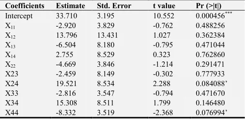
Using the data in table 1, and the model (9), ANOVA was run using R software. This was done to find how different blend at the design points contribute to the response variable when the mean productivity measured by the intercept of the model is taken into account. The following result were obtained
Residuals on the responses:
(57)
Table 2. ANOVA Table Showing the Significance of the Design Points.
Coefficients Estimate Std. Error t value Pr (>|t|) Intercept 33.710 3.195 10.552 0.000456*** X11 -2.920 3.829 -0.762 0.488256 X12 13.796 13.431 1.027 0.362384 X13 -6.504 8.180 -0.795 0.471044 X14 2.755 8.529 0.323 0.762860 X22 -4.669 3.846 -1.214 0.291471 X23 -2.459 8.149 -0.302 0.777933 X24 19.521 8.534 2.288 0.084088’ X33 -2.816 3.547 -0.794 0.471670 X34 15.308 8.511 1.799 0.146480 X44 -8.332 3.519 -2.368 0.076994’
Signif. codes: 0.001 ‘***’, 0.01 ‘**’, 0.05 ‘*’, 0.1’. Residual standard error: 1.526 on 4 degrees of freedom Multiple R-squared: 0.9275, Adjusted R-squared: 0.7464 F-statistic: 5.12 on 10 and 4 DF, p-value: 0.06475
From this table which shows the result of ANOVA, it can be seen that by introducing the constant which is measured by the intercept. Then we increased the precision of our estimates as shown by the adjusted R-squared compared with (55). This implies other feeding practices except the supplement have significant impacts on variation to milk productivity.
Also the blend of 2
x (Soya beans) and 4
x (Fish meal) shows significance at 0.1, this implies that this blend contribute significantly to milk productivity.
A blend of 44
x (fish meal) shows significance at 0.1, implying that fish meal supplement is significance in milk productivity.
4. Conclusions and Recommendations
4.1. Conclusions
In this study, the following conclusions were drawn. a. The derivation of the Kronecker model involved a
subsystem of interest which was used to derive the
coefficient matrix. We averaged the interaction of ingredients from the full parameter system to derive our subsystem of interest vector. In determining the coefficient matrix for the Kronecker model, the research recommends that other combinations of ingredients can be done to determine a different vector of the subsystem of interest.
b. The fitted Kronecker model support the result of the polynomial model. From the computed adjusted R2 we conclude the model provides a good fit and F-ratio support that supplement are significant in explaining the variation in milk production. The ANOVA summaries, proves that by introducing the constant which is measured by the intercept we make our estimate more precise as the adjusted R2 is improved. This implies other feeding practices except the supplement have significant impacts on variation to milk productivity. c. The results also show that the blend of Soya beans and
Fish meal contribute significantly to milk productivity. Also pure blend of fish meal supplement is significance in milk productivity. The research therefore, recommends this supplement for optimal milk productions.
4.2. Recommendations
From this study we recommend the following:
a. For dairy farmers to achieve most optimal production, they need to blend feeds supplement with at least three of the ingredients.
b. As stated in chapter 3, the researcher recommends that further studies should be done on milk productivity of dairy animals across the bleed given meal concentrates as supplement. This will be aimed at reducing variability in the model. This is guided by the assumption that different blend of concentrates may affect production differently across the breeds of dairy cows.
References
[1] J. A. Cornell. (2002). Experiments with Mixtures, Third Edition. John Wiley, New York.
[2] J. Wegner & T. Stanton. (2006). Formulating ratios with Pearson square.
http/www.ext.colostateedu.Pubs/livestock/01618.html [3] R. Rossi. (2004). Least cost formulation software: An
introduction section: feature articles, Aqua feeds: formulation and beyond 3: 3-5.
[4] R. G. Muriungi, J. K. Koske & J. M. Mutiso. (2017). Applying the Polynomial Model in Simplex- Centroid design to formulate the Optimum Dairy Feed. International Journal of Sciences: Basic and Applied Science. ISSN 2307-4531. PP. 101-117.
[5] R. H. Myres, D. C. Montgomery, & C. M. Anderson. (2009), Response Surface Methodology, Wiley and sons, Hoboken New Jersey
[6] G. W. Dean, D. L. Bath, & S. Olayada, (1969). Computer program for maximizing income above feed cost from dairy cattle. American science association journal
[7] S. Chakeredza, F. K. Akinnifesi, C. O. Ajayi, G. Sileshi, S. Mngomba, & F. Gondwe. (2008), A simple method of formulating least-cost diets for smallholder dairy production in Sub-Saharan Africa. African journal of Biotechnology Vol 7 (16), pp 2925-2933
[8] D. Mahmut, S. T. Omer, A. Tugba, & G. Meryem. (2013) Optimization of Gum Combination in Prebiotic Instant Hot Chocolate Beverage Model System in terms of Rheological
Aspect: Mixture Design Approach. Journal of Food and Bioprocess Technology Vol 6 pp 783-794
[9] L. C. Okpala, & E. C. Okoli. (2013) Optimization of Composite Biscuits Flour by Mixture Response Surface Methodology. Food Science and Technology International 19(4).
[10] L. Shuanzhe, & N. Heinz. (1995) A V-optimal design for Scheffe polynomial model. Statistics and Probability Letters 23, pg 253-258
[11] J. K. Koske, J. K. Kinyanjui, J. M. Mutiso, & M. R. Cherutich. (2009), Designs with optimal values in the second degree Kronecker non-maximal model mixture experiments. American Journal of Mathematics and Mathematical Sciences vol 1 no. 2 pp 155-160.
[12] D. W. Gaylor & H. C. Sweeny. (1965). Design for Optimal Prediction in Simple Linear Regression. Journal of the American Statistical Association. Vol 60, 1965 no. 309 pp 205-216.
[13] R. L. J. Coetzer, & W. W. Focke. (2010). Optimal designs for estimating the parameters in weighted power-mean mixture models.
[14] N. R. Draper, & F. Pukelsheim. (1999). Kiefer ordering of simplex designs for first- and second-degree mixture models. Journal of statistical planning and inference, 79, 325-348
[15] N. R. Draper, B. Heiligers, & P. Pukelsheim. (1998). Kiefer ordering of simplex designs for second-degree mixture models with four or more ingredients. Annals of statistics vol 28 no. 2 pg 578-590