Forecasting Temperatures in Bangladesh: An Application
of SARIMA Models
Md. Siraj Ud Doulah
Department of Statistics, Begum Rokeya University, Rangpur, Bangladesh. E-mail: [email protected]
Climate change is presently among the significant topics of discussion and temperature is one of its main components. In this study, it is to be observed that the minimum temperature is more fluctuating compared to the maximum temperature. Several suggested SARIMA models were established for maximum and minimum temperature series according to the methods of the Box
Jenkin’s methodology. The best model for maximum temperature is SARIMA (1, 0, 0) (1, 1, 0)12
and for minimum temperature is SARIMA (2, 0, 1) (2, 1, 0)12 selected based on AIC. From the model
validation outcomes, the projected values are well-fitted through the original data with the lower and upper limits holding bulks of the original data. The detected models are therefore suitable to be used for projecting monthly maximum and minimum temperature in Bangladesh. The selected SARIMA models give two-year predicted monthly maximum and minimum temperatures that can help decision makers to establish priorities for preparing themselves against forthcoming weather fluctuations. The forecasts also display that the minimum temperature of Bangladesh will continue with the upward trend. This is a reflection of a fluctuating climate in the entire country.
Keywords: Temperature, SARIMA, Validation, Forecasting, Bangladesh
INTRODUCTION
The most influential factors in the climate are temperature and moisture. According to a study by Oluwafemi et al. (2010), climate change seems to be one of the most important issues in the recent two decades and temperature has been identified as one of the key elements that can indicate climate change. The gradual rise in the mean temperature of the Earth’s atmosphere and its oceans is referred to as Global warming. It is widely believed that the changing temperature due to global warming is permanently changing the entire Earth’s climate. For a long time, the biggest debate in a number of local and international forums worldwide has been whether global warming is real which is described in (Nigar and Mahedi, 2015). Some people think that global warming is not real. However, several climate scientists have carried out researches and have come to a conclusion that the globe is gradually warming. People perceive the impacts of global warming differently with some taking the necessary precautions to help reduce the rates of the rising temperatures. Increase in temperatures are likely to lead to a global increase in drought conditions, decreased water supplies due to evapotranspiration and an increase in urban and agricultural demand. Vital sectors of the Bangladesh economy like Agriculture greatly rely on climate. Plants can grow only within certain limits of
temperature. Each plant species has an optimal temperature limit for its different stages of growth and functions which are described in (Syeda, 2012). They also have an upper and lower lethal limits between which they can properly grow. Temperature determines which species can survive in a particular region. Several farmers are however unaware of the changing climate and are also ignorant of the adverse impacts it will have on their livelihoods. High temperatures causes prolonged droughts, affects the amount of water in the soil, affects rainfall patterns and reduces water catchment areas. The increased temperatures can also cause an outbreak of pests and diseases that affects plants, animals and humans. Farmers who are aware of the changing climate are also helpless and unaware of what to do. They continue with poor agricultural practices like burning of wastes and poor disposal of unused fertilizers that worsen the situation by releasing greenhouse gasses to the atmosphere. Studying temperature changes is thus vital for the Bangladesh economy as Agriculture which is the country’s largest source revenue is directly affected by the rising temperatures. The Bangladesh government derives nearly 20% of its revenue from the agricultural sector. As the largest employer in the economy, the agricultural sector accounts for about 50% of the country’s
International Journal of Statistics and Mathematics
Vol. 5(1), pp. 108-118, September, 2018. © www.premierpublishers.org. ISSN: 2375-0499
employment. In addition, more than 70% of Bangladesh population living in rural areas depends on agricultural related activities for their daily livelihoods. Climatic studies on temperature are therefore vital for the survival of the agricultural sector as the key source of revenue to the government of Bangladesh.
Temperature is one of the key elements of climate and it is important to various sectors of the economy like Agriculture. Temperature affects water sources, pests that attack plants, animals and human diseases. Despite the increasing climate changes, majority of Bangladeshi citizens are still not well informed. Analyzing and forecasting of temperature changes will thus help various stakeholders and government to plan in advance in order to counter climate related disasters. The objective of this research is to build a time series model and use this model to analyze and forecast the variation in maximum and minimum temperature in Bangladesh in order to inform stakeholders who depend directly or indirectly on it to plan in advance.
METHODOLOGY
Average Maximum and Minimum Monthly temperature data covering Bangladesh has been collected from the Bangladesh Meteorological Department (BMD). This data was recorded in monthly basis covering an 18 year period from January 2000 to December 2017 (www.data.gov.bd). The temperatures are measured in degrees Celsius.The temperature data is a continuous univariate time series as it contains a single variable (temperature) which is measured at every instant of time. However, this data was merged into monthly intervals transforming it to a discrete univariate time series.
The Box-Jenkins Method
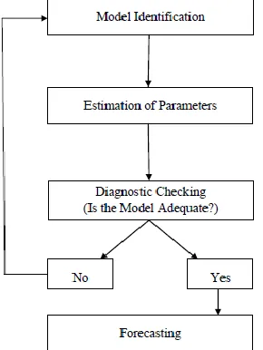
This study follows the Box-Jenkins methodology for modeling. The following conceptual framework proposed by Box et al. (1976) is considered in this study.
Figure 1. Box- Jenkins ARIMA Model
Seasonal ARIMA (SARIMA) Model
Gurudeo and Mahbub (2010) alludes that most natural factors like temperature have strong seasonal Components. It is therefore necessary to use autoregressive and moving average polynomials that identify with the seasonal lags. One such model is the SARIMA model. SARIMA model is an extension of ARIMA model and it is applied when the series contains both seasonal and non-seasonal behavior. SARIMA model is sometimes called the multiplicative seasonal autoregressive integrated moving average and is denoted by SARIMA (p,d,q)(P,D,Q)S. The Seasonal AR can be written as:
t t s
p
B
y
(
)
The Seasonal MA can be written as
t s Q
t
B
y
(
)
The seasonal differencing is expressed as
s t t t s
y
y
y
B
)
1
(
Combining the above equations, we get SARIMA
t s Q q t
D s d s
p
p
B
B
B
B
y
B
B
(
)
(
)(
1
)
(
1
)
0
(
)
(
)
Where the constant equals
)]
1
)(
1
[(
1 10
p
p
Where p represents non-seasonal AR order, d represents non seasonal differencing, q represents non seasonal MA order, P represents seasonal AR order, D represents seasonal differencing, Q represents seasonal MA order, S represents seasonal order (for monthly data S = 12 )
y
t represents time series data at period t, B is the backward shift operator (B y
k t
y
t k ) and
tis the random shock(white noise error).
Stationarity Analysis
is non-stationary, at least in the mean value. Here we applied most widely used popular formal test over the past several years are Autocorrelation function (ACF), Partial Auto-correlation function (PACF), augmented dickey-fuller (ADF) test and Kwiatkowski, Phillips, Schmidt and Shin (KPSS) test.
Autocorrelation and Partial Autocorrelation (ACF and PACF) Functions
When using the SARIMA models, Model specification and selection is a crucial step of the analysis process. A proper model for the series is identified by analyzing the ACF and PACF. They reflect how the observations in a time series are related to each other. It is useful that the ACF and PACF are plotted against consecutive time lags for the purposes of modeling and forecasting (Brockwell, 2002). The order of the AR and MA are determined by these plots. For a time series, the auto-covariance function ACVF at lag k is defined as:
n kt
k t t
k
n
y
y
c
1
)
)(
(
1
If
x
tis a stationary process with mean μ, the autocorrelation of order k is simply the relation betweeny
t andy
tk. The ACF estimate for the sample at lag k is thus defined as)}
{(
)}
)(
{(
t k t t ky
E
y
y
E
The PACF of a stationary process
y
t denoted
hh is)
1
(
)
,
(
1 11
corr
y
ty
t
,
3
,
2
,
1
ˆ
1 1 1 1 1 , 1
p
r
r
r
p j j pj p j j p pj p p p
Where,
ˆ
p1,j
ˆ
pj
ˆ
p1,p1
ˆ
p,pj1The ACF and PACF plots are used to identify the terms of the SARIMA model.
ADF & KPSS Tests
Stationarity can also be checked using Augmented Dickey Fuller (ADF) & Kwiatkowski–Phillips–Schmidt–Shin (KPSS) tests. The literatures of these tests are described in many textbooks (Corliss, 2009; Chris, 2004; Spyros, 1998).
Augmented Dickey-fuller (ADF) test
Testing for a unit root is equivalent to testing
1
in the following modelADF test equation:
t j t p j j t
t
Y
Y
Y
01 1 1
)
1
(
t j t p j j tt
Y
Y
Y
01 1 1 Hypothesis
1
:
0
H
1
|
|
:
1
H
Reject
H
0ift
1
Critical
Value
Or
0
:
0
H
0
:
1
H
Reject
H
0ift
0
Critical
Value
The ADF the test statistic has same asymptotic distribution as the DF statistic, so the same critical values can be used.
Kwiatkowski–Phillips–Schmidt–Shin (KPSS) test
To be able to test whether we have a deterministic trend vs stochastic trend, we are using KPSS (Kwiatkowski, Phillips, Schmidt and Shin) Test (1992).
)
0
(
~
:
0
Y
I
H
t Level (or trend) stationary
)
1
(
~
:
1
Y
I
H
t Difference stationarySTEP 1: Regress
Y
t on a constant and trend and construct the OLS residuals
(
1,
2,
,
T)
STEP 2: Obtain the partial sum of the residuals.
T t t tS
1
STEP 3: Obtain the test statistic
T t tS
T
KPSS
1 2 2 2ˆ
where
ˆ
2 is the estimate of the long-run variance of the residuals.STEP 4: Reject
H
0 when KPSS is large, because that is the evidence that the series wander from its mean. It is the most powerful unit root test but if there is a volatility shift it cannot catch this type non-stationarity.Model selection criterion
states that the motivation behind the selection criteria of the model is to identify the best model that neither under-fits nor over-under-fits the data.
Model Diagnostic
Here, each selected model is assessed to determine how well it fits the temperature data. For a model that fits the data well, Ljung-Box test based on ACF and PACF of the residuals are used in determining the goodness of fit of the selected model which is discussed in (Chris, 2004). The Ljung-Box test is defined below-
0
H
: the model does not exhibit lack of fit1
H
: the model exhibit lack of fit The test statistic is defined as:
mk k
k
n
r
n
n
Q
1 2
ˆ
)
2
(
Where,
r
ˆ
k is the estimated autocorrelation of the series at lag k, m is the number of lags being tested, n is the sample size. The statisticQ
follows a
( )2m . For a level of significance α, the critical region for rejection of the hypothesis isQ
(12, )m where m is the degrees of freedom.Forecasting
Forecasting is important in decision making process (Brockwell et al. 2002; Box et al. 1976). The chosen model should therefore produce accurate forecasts. The selected model does not always necessarily provide the best forecasting therefore it is important to apply other tests such as MAE, MSE and MAPE to confirm the forecasting accuracy of the model.
Forecasting an ARMA process with mean
y, m-step-ahead forecasts can be defined asj m n m j
j y
m n
y
The precision of the forecast is assessed with a prediction interval of the form
n m n n
m
n
C
P
y
2
Where 2
C
is identified such that the desired degree of confidence is achieved. Suppose it is Gaussian process, then having2
2
C
will yields approximately 95%prediction interval for
y
nm.Data Analysis
The statistical software R package has been used in this analysis. The results and discussions of the temperatures data set are shown in the following below:
Figure 2: Time plot of Maximum and Minimum
temperatures
From Figure 2, it is to be noted that there is no evidence of systematic variation about the mean on the time series plot for maximum and minimum temperatures. For both temperatures, it is clear that the series is non stationary. However, both series exhibit seasonality which is evident from the strong yearly cycles.
Table 1: Summary statistics of maximum and minimum temperatures
Temperature
(°C) Range
Minimum Value
Maximum
Value Mean
Standard
Deviation Variance Maximum 11.9 23.02 34.92 30.7 2.7 7.3 Minimum 15.8 11.09 26.86 21.4 4.8 23.2
From Table 1, it is observed that the minimum temperature is more varying (standard deviation=4.8) compared to the maximum temperature (standard deviation=2.7).
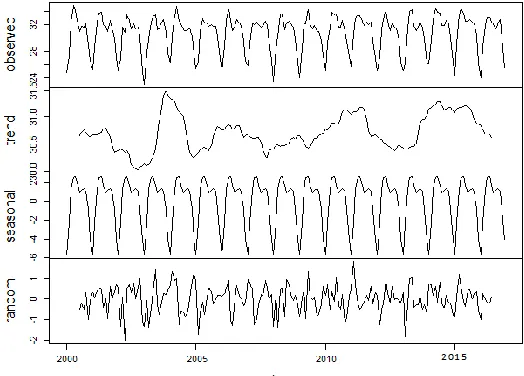
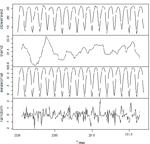
Figure 4. Decomposition of Minimum temperature
Ordinarily, time series data exhibit trend, seasonal, cyclical and random components. From Figure 3 & Figure 4, it is evident that both maximum and minimum temperature series have seasonal, random and trend components. The upward trend is clearly evident for the minimum temperature series.
Stationarity checking
Why are stationary time series so important? Because if a time series is non-stationary, we can study its behavior only for the time period under consideration. Each set of time series data will therefore be for a particular episode. As a consequence, it is not possible to generalize it to other time periods. Therefore, for the purpose of forecasting, such (non-stationary) time series may be of little practical value. How do we know that a particular time series is stationary? There are several tests of stationary. Here we used graphical and analytical recognized test.
Maximum temperature
Minimum temperature
Figure 5: Autocorrelation and Partial Autocorrelation function
From Figures 5, it is to be exhibited the plots of the ACFs and the PACFs for the monthly maximum and minimum temperature series. The plots show strong seasonal wave patterns that decline moderately. The non-seasonal lags decay rapidly. This confirms the presence of seasonality behavior and thus the time series is non-stationary. Therefore, from the time series and autocorrelation plots, it is obvious that both maximum and minimum temperature series have seasonal variation. To make the series stationary, seasonal differencing is required.
Formal tests of Stationarity are performed next to confirm the conclusions from visual inspection of seasonal and non-seasonal Stationary.
Table 2: Augmented Dickey – Fuller (ADF) Test
Temperatures Dickey-Fuller
Lag order
Critical Value
p-value Maximum -2.8429 12 0.05 .2229 Minimum -2.4787 12 0.05 .3755
According to the ADF tests results for both maximum and minimum temperature series shown in Table 2, we do not reject the null hypothesis and conclude that the two series are not stationary. This is because the more negative the Dickey –Fuller is, the stronger the rejection of the null hypothesis which is not the case here.
Table 3: KPSS Test Temperatures KPSS
level
Lag parameter
Critical Value
temperature series we do not reject the null hypothesis because the p-value of 0.1 ≥ 0.05 at 5% level of significance. Thus the maximum temperature is trend stationary. From the results, for minimum temperature series we do not reject the null hypothesis because the p-value of 0.1 ≥ 0.05 at 5% level of significance. Thus the minimum temperature is trend stationary.
Model building for monthly temperature series
According to Shumway and Stoffer (2006), the process of model fitting involves data plotting, data transformation if necessary, Identification of dependence order, estimation of parameter, diagnostic analysis and choosing appropriate model. In this section, a univariate SARIMA methodology is used to model maximum and minimum monthly temperatures of Bangladesh.
Model Identification
ACF and PACF plots are used in the identification of the values p, q, P and Q. For the non-seasonal part, spikes of the ACF at low lags are used to identify the value of q while the value of p is identified by observing the spikes at low lags of the PACF. For the seasonal part the value of Q is observed from the ACF at lags that are multiples of S while for P, the PACF is observed at lags that are multiples of S. Looking at the ACF plots and PACF plots for maximum and minimum differenced time series, the models are suggested in the following Table 4.
Table 4: Suggested Models
Maximum temperature Minimum temperature SARIMA (0, 0, 0) (0, 1, 0)12 SARIMA (2, 0, 2) (1, 1, 0)12
SARIMA (0, 0, 1) (0, 1, 0)12 SARIMA (0, 0, 0) (0, 1, 0)12
SARIMA (1, 0, 0) (0, 1, 0)12 SARIMA (1, 0, 0) (1, 1, 0)12
SARIMA (0, 0, 1) (1, 1, 0)12 SARIMA (2, 0, 1) (1, 1, 0)12
SARIMA (1, 0, 0) (1, 1, 0)12 SARIMA (2, 0, 1) (2, 1, 0)12
Analyzing the aforementioned models for both Maximum & Minimum temperatures, the results of the estimated models are shown in the following Table 5.
Table 5: Suggested Models Estimation Results Maximum temperature
Model P-value
Chi-square DF AIC
SARIMA (0, 0, 0) (0, 1, 0)12 3.49e-07 40.582 6 592.35
SARIMA (0, 0, 1) (0, 1, 0)12 .03504 13.544 6 574.97
SARIMA (1, 0, 0) (0, 1, 0)12 .174 8.993 6 569.15
SARIMA (0, 0, 1) (1, 1, 0)12 .0963 10.754 6 532.07
SARIMA (1, 0, 0) (1, 1, 0)12 .3157 7.0564 6 527.79
Minimum temperature
Model P-value
Chi-square
DF AIC
SARIMA (2, 0, 2) (1, 1, 0)12 .3899 6.3049 6 526.6
SARIMA (0, 0, 0) (0, 1, 0)12 .00153 21.412 6 557.52
SARIMA (1, 0, 0) (1, 1, 0)12 .3157 7.0564 6 527.79
SARIMA (2, 0, 1) (1, 1, 0)12 .3521 6.673 6 531.37
SARIMA (2, 0, 1) (2, 1, 0)12 .7639 3.349 6 505.45
The best model is the one with the lowest value of AIC. From Table 5, it is to be noted that the best model for maximum temperature is SARIMA (1, 0, 0) (1, 1, 0)12 while
for minimum temperature is SARIMA (2, 0, 1) (2, 1, 0)12.
The lowest value of AIC is 527.79 and the Ljung -Box test yielded a chi square of 7.0564 with a p value equal to 0.3157. From the Ljung -Box test, the p value of 0.3157 > 0.05 and this confirms that SARIMA (1, 0, 0) (1, 1, 0)12 is
adequate for forecasting of maximum temperature. The lowest value of AIC is 505.45. and the Ljung -Box test yield a chi square of 3.349 with a p value of 0.7639. From the Ljung -Box test, the p value of 0.7639 > 0.05 and this confirms that SARIMA (2, 0, 1) (2, 1, 0)12 is adequate for
forecasting of minimum temperature.
Parameter Estimation
Non-linear least-squares estimation or Maximum likelihood estimation methods are employed to estimate the coefficients of the models. A more complicated iteration procedure is required when estimating the parameters of SARMA models (Box et al. 1976; Chris 2004).
Table 6: Select models Parameter Estimates Results Model SARIMA (1, 0, 0) (1,
1, 0)12 for Maximum
temperature
Model SARIMA (2, 0, 1) (2, 1, 0)12 for Minimum
temperature Parameter Estimate Std.
error
Parameter Estimate Std. error AR(1) .3476 .0675 AR(1) -.6536 .0706 SAR(1) -.4498 .0633 AR(2) .2717 .0702 MA(1) 1.00 .0166 SAR(1) -.6165 .0689 SAR(2) -.3595 .0694
From Table 6 we observed that the models are estimated well because of very low standard error of the estimated parameters.
Diagnostic Analysis
For a well fitted models, for maximum temperature is SARIMA (1, 0, 0) (1, 1, 0)12 while for minimum temperature
is SARIMA (2, 0, 1) (2, 1, 0)12, the standardized residuals
Figure 6: Selected Model Residuals Q-Q Plot for Maximum Temperature
A normal probability plot or a Q-Q plot can help in identifying departures from normality. From figure 6, the residuals are approximately normal distributed with zero mean.
Figure 7: Selected Model Residuals Plots for Maximum Temperature
From Figure 7, it is to be observed three different plots such as standardized residuals; ACF of residuals and p-values for Ljung –Box statistic. Based on standardized residuals plot, it looks like an independently and identically distributed sequence of mean zero with a constant variance. The plots of the ACF of the residuals lack enough evidence of significant spikes which clearly shows that the residuals are white noise. The results also showed that the residuals are non-significant with Ljung –Box test p-value. From the above tests, it is clear that the fitted model is adequate since the residuals are white noise. That is,
SARIMA (1, 0, 0) (1, 1, 0)12 is adequate for modeling the
monthly maximum temperature series in Bangladesh.
Figure 8: Selected Model Residuals Q-Q Plot for Minimum Temperature
From Figure 8, we observed that the residuals are approximately normal distributed with zero mean and constant variance.
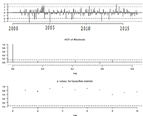
Figure 9: Selected Model Residuals Plots for Minimum Temperature
shows that the residuals are white noise. The results also showed that the residuals are non-significant with Ljung – Box test p-value. From the above tests, it is clear that the fitted model is adequate since the residuals are white noise. That is, SARIMA (2, 0, 1) (2, 1, 0)12.is adequate for
modeling the monthly minimum temperature series in Bangladesh.
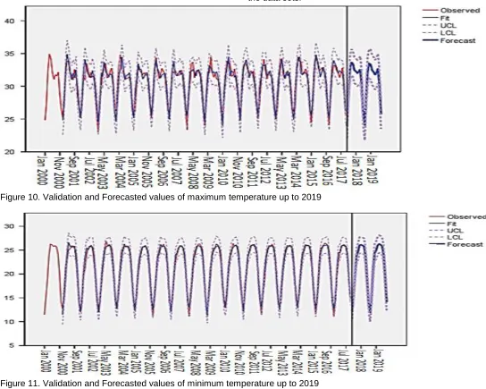
Model validation & Forecasting
In order to test the adequacy and predictive ability of the chosen models, the actual data sets, predicted values, lower and upper limits are plotted and displayed in Figure 10 & 11. The graphs show that the predicted values are well-fitted through the original data with the lower and upper limits containing majorities of the original data. This indicates that the models chosen for maximum and minimum temperature series are the best fitted ones for the data sets.
Figure 10. Validation and Forecasted values of maximum temperature up to 2019
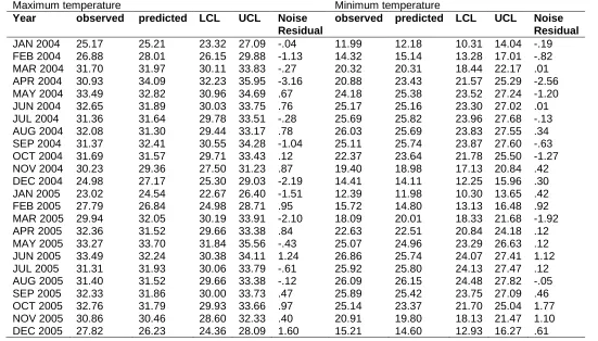
From Table 7, it is to be remarkable that the observed values verses the predicted values as well as the noise residuals that affirms the adequacy of the chosen maximum and minimum time series models.
Table 7: Observed and fitted values for the Period 2004-2005
Maximum temperature Minimum temperature
Year observed predicted LCL UCL Noise
Residual
observed predicted LCL UCL Noise
Residual
JAN 2004 25.17 25.21 23.32 27.09 -.04 11.99 12.18 10.31 14.04 -.19 FEB 2004 26.88 28.01 26.15 29.88 -1.13 14.32 15.14 13.28 17.01 -.82 MAR 2004 31.70 31.97 30.11 33.83 -.27 20.32 20.31 18.44 22.17 .01 APR 2004 30.93 34.09 32.23 35.95 -3.16 20.88 23.43 21.57 25.29 -2.56 MAY 2004 33.49 32.82 30.96 34.69 .67 24.18 25.38 23.52 27.24 -1.20 JUN 2004 32.65 31.89 30.03 33.75 .76 25.17 25.16 23.30 27.02 .01 JUL 2004 31.36 31.64 29.78 33.51 -.28 25.69 25.82 23.96 27.68 -.13 AUG 2004 32.08 31.30 29.44 33.17 .78 26.03 25.69 23.83 27.55 .34 SEP 2004 31.37 32.41 30.55 34.28 -1.04 25.11 25.74 23.87 27.60 -.63 OCT 2004 31.69 31.57 29.71 33.43 .12 22.37 23.64 21.78 25.50 -1.27 NOV 2004 30.23 29.36 27.50 31.23 .87 19.40 18.98 17.13 20.84 .42 DEC 2004 24.98 27.17 25.30 29.03 -2.19 14.41 14.11 12.25 15.96 .30 JAN 2005 23.02 24.54 22.67 26.40 -1.51 12.39 11.98 10.30 13.65 .42 FEB 2005 27.79 26.84 24.98 28.71 .95 15.72 14.80 13.13 16.48 .92 MAR 2005 29.94 32.05 30.19 33.91 -2.10 18.09 20.01 18.33 21.68 -1.92 APR 2005 32.36 31.52 29.66 33.38 .84 22.63 22.51 20.84 24.18 .12 MAY 2005 33.27 33.70 31.84 35.56 -.43 25.07 24.96 23.29 26.63 .12 JUN 2005 33.49 32.24 30.38 34.11 1.24 26.86 25.74 24.07 27.41 1.12 JUL 2005 31.31 31.93 30.06 33.79 -.61 25.92 25.80 24.13 27.47 .12 AUG 2005 31.40 31.52 29.66 33.38 -.12 26.09 26.15 24.48 27.82 -.05 SEP 2005 32.33 31.86 30.00 33.73 .47 25.89 25.42 23.75 27.09 .46 OCT 2005 32.76 31.79 29.93 33.66 .97 25.14 23.37 21.70 25.04 1.77 NOV 2005 30.86 30.46 28.60 32.33 .40 20.91 19.80 18.13 21.47 1.10 DEC 2005 27.82 26.23 24.36 28.09 1.60 15.21 14.60 12.93 16.27 .61
Forecasting
Forecasting helps in planning and decision making process since it gives an insight of the future uncertainty using the past and current behavior of given observations. Further accuracy tests such as MAE, MAPE and RMSE must therefore be carried out on the model. The Table 8 shows a summary of ME, RMSE and MAE for both maximum and minimum temperature models.
Table 8: Forecasting Accuracy Statistic
Maximum temperature model SARIMA (1, 0, 0) (1, 1, 0)12
Minimum temperature model SARIMA (2, 0, 1) (2, 1, 0)12
Stationary R-squared .304 .314
R-squared .877 .968
RMSE .949 .867
MAPE 2.378 3.362
MAE .716 .622
Here, it is to be forecasted the monthly temperature based on the selected models SARIMA (1, 0, 0) (1, 1, 0)12 for maximum
Table 9: Forecasting Monthly temperatures
Maximum temperature Minimum temperature
95% CI 95% CI
Year Forecast LCL UCL Forecast LCL UCL JAN 2018 23.95 22.09 25.82 12.25 10.58 13.92 FEB 2018 28.80 26.83 30.78 15.30 13.62 16.97 MAR 2018 32.60 30.61 34.58 20.14 18.45 21.83 APR 2018 33.69 31.70 35.67 23.86 22.16 25.55 MAY 2018 33.43 31.45 35.42 24.70 23.01 26.40 JUN 2018 32.46 30.48 34.45 26.03 24.33 27.72 JUL 2018 32.27 30.29 34.26 26.12 24.43 27.81 AUG 2018 32.02 30.04 34.01 25.97 24.27 27.66 SEP 2018 32.20 30.21 34.19 25.80 24.11 27.50 OCT 2018 32.59 30.60 34.58 23.80 22.10 25.49 NOV 2018 30.13 28.15 32.12 18.91 17.21 20.60 DEC 2018 25.89 23.91 27.88 14.04 12.35 15.74 JAN 2019 24.01 21.77 26.24 11.87 10.03 13.71 FEB 2019 28.79 26.53 31.06 15.21 13.37 17.05 MAR 2019 32.27 30.00 34.54 20.85 19.01 22.69 APR 2019 33.45 31.18 35.71 24.45 22.61 26.29 MAY 2019 33.32 31.05 35.59 24.93 23.09 26.77 JUN 2019 32.44 30.18 34.71 25.99 24.15 27.83 JUL 2019 32.20 29.93 34.46 26.27 24.43 28.11 AUG 2019 31.73 29.46 34.00 26.14 24.29 27.98 SEP 2019 32.12 29.86 34.39 25.82 23.98 27.66 OCT 2019 32.70 30.43 34.96 24.15 22.30 25.99 NOV 2019 30.03 27.76 32.30 19.33 17.49 21.17 DEC 2019 25.74 23.47 28.00 14.10 12.26 15.94
CONCLUSIONS
To sum up the whole discussion it is to be noteworthy that for both maximum and minimum temperatures are unsteady from month to month though the maximum temperature is more fluctuating (standard deviation=2.7) compared to the minimum temperature (standard deviation=4.8). However, through the years, there is a distinct increasing trend for minimum temperature proving the fact that global warming is in fact a reality. On the other hand, maximum temperatures seem to be comparatively steady. Both maximum and minimum temperature series exhibited high seasonality. The minimum temperature also displayed an upward trend. The two series were made stationary. The best model for maximum temperature is SARIMA (1, 0, 0) (1, 1, 0)12 and for minimum temperature
is SARIMA (2, 0, 1) (2, 1, 0)12. The model residuals for both
series are near normality as most points fall on the straight line with a few close to it. From the model validation results, the projected values are well-fitted through the original data with the lower and upper limits encompassing bulks of the original data. The selected SARIMA models give two-year projected monthly maximum and minimum temperatures that can help decision makers to establish priorities for equipping themselves against upcoming weather changes. The forecasts also show that the minimum temperature of Bangladesh will continue with the upward trend.
ACKNOWLEDGEMENTS
The author would like to thank the anonymous reviewers for their helpful comments.
REFERENCES
Aidoo E (2010). Modeling and forecasting inflation rates in Ghana: An application of SARIMA models. Högskolan Dalarna, School of Technology and Business Studies. Brockwell, Peter J, Davis RA (2002). Introduction to Time
Series and Forecasting, 2nd.edn. Springer-Verlang. Box GEP, Jenkins GM, Reinsel GC (1976). Time Series
Analysis, Forecasting and Control, 3rd edn. Prentice Hall, Englewood Clifs, NJ.
Burnham KP, Anderson DR (1998). Model Selection and Inference. Springer Verlag, New York.
Corliss D (2009). Time series Analysis: an introduction using Base SAS and STAT,NewYork, U.S.A.
Chris C (2004). The Analysis of Time Series: An Introduction, John Wiley & Sons, NewYork, U.S.A. Gurudeo AT, Mahbub I. (2010). “Time Series Analysis of
Rainfall and Temperature Interactions in Coastal Catchments”, J of Math. and Stat. 6 (3): 372-380. Nigar S, Mahedi H. (2015). Forecasting Temperature in
Oluwafemi SO, Femi JA, Oluwatosi TD. (2010). Time Series Analysis of Rainfall and Temperature in South West Nigeria, The Pacific J. of Sci. and Techno. 11(2):552-564.
Syeda J. (2012). Trend and Variability Analysis, and Forecasting of Maximum Temperature in Bangladesh, J. Environ. Sci. & Natural Resources. 5(2): 119 -128. Spyros M, Wheelwright SC, Hyndman RJ (1998).
Forecasting: Methods and Applications, John Wiley & Sons, Inc., U.S.A.
Shumway RH, and Stoffer DS (2006). Time Series Analysis and Its Applications With R Examples, Springer Science & Business Media, LLC, NY, USA.
www.data.gov.bd
Accepted 5 September 2018
Citation: Doulah S. (2018). Forecasting Temperatures in Bangladesh: An Application of SARIMA Models. International Journal of Statistics and Mathematics, 5(1): 108-118.