VOLUME 38, ARTICLE 59, PAGES 1815
,
1842
PUBLISHED 7 JUNE 2018
http://www.demographic-research.org/Volumes/Vol38/59/ DOI: 10.4054/DemRes.2018.38.59
Research Article
The effects of family and location on wealth:
A longitudinal study of the US North, 1850–1870
Alice Kasakoff
Andrew Lawson
Purbasha Dasgupta
Michael DuBois
Stephen Feetham
This publication is part of the Special Collection on “Spatial analysis in historical demography: Micro and macro approaches,” organized by Guest Editors Martin Dribe, Diego Ramiro Fariñas, and Don Lafreniere.
© 2018 Alice Kasakoff et al.
T This open-access work is published under the terms of the Creative Commons Attribution 3.0 Germany (CC BY 3.0 DE), which permits use, reproduction, and distribution in any medium, provided the original author(s) and source are given credit.
1 Introduction 1816
2 Inequality and mobility in the region 1817
2.1 Economic context 1817
2.2 Wealth differences between counties: Bayesian spatial analysis 1818
3 The genealogical sample 1819
4 Individual real property in the US North: 1850 to 1870 1820
4.1 Wealth 1820
4.2 The completer sample 1821
5 Bayesian analysis 1823
5.1 Spatial and family effects 1823
5.1.1 Models 1823
5.1.2 Results 1826
5.2 Wealth of fathers and sons 1828
6 Moving and occupational changes 1830
7 Discussion 1831
7.1 Spatial and temporal effects 1831
7.2 Family effects 1832
8 Conclusions 1833
9 Acknowledgements 1834
References 1835
The effects of family and location on wealth:
A longitudinal study of the US North, 1850–1870
Alice Kasakoff1
Andrew Lawson2 Purbasha Dasgupta3
Michael DuBois4
Stephen Feetham5
Abstract
BACKGROUND
Family effects can be confounded with spatial effects, since family members live near each other.
OBJECTIVE
Our aim is to find out whether a father’s wealth was related to his son’s wealth when spatial effects are included in the model. The data is from the United States from 1850 to 1870. Since the data comes from genealogies we are also able to test for deeper family effects lasting several generations.
METHODS
This article uses Bayesian longitudinal methods that incorporate spatial effects. The data comes from the genealogies of nine New England families that have been linked to the US censuses of 1850, 1860, and 1870, which had information on real property, the dependent variable in our analysis.
RESULTS
No relationship was found between the wealth of the father and his sons in our data, nor were the deeper family effects significant. Spatial effects were also not significant.
1 Department of Geography, University of South Carolina, Columbia, South Carolina, USA. Email: [email protected].
2 Department of Public Health Sciences, Medical University of South Carolina, Charleston, South Carolina,
USA.
3 United Way of Central Indiana, Indianapolis, Indiana, USA. 4 York County (South Carolina) Government, York, USA.
However, there was a strong temporal effect: Men were wealthier in 1860 than they were in 1850 or 1870.
CONCLUSION
There is evidence of economic mobility in a rapidly expanding population and economy
such as the United States was during the 19th century. Since temporal effects were more
important than spatial effects the amount of mobility might be transitory and highly dependent upon the particular time period and cohort being studied.
CONTRIBUTION
The article illustrates the usefulness of methods that include spatial effects for the study of economic mobility, particularly in studies of family effects, and the importance of including both spatial and temporal effects when analyzing economic mobility.
1. Introduction
Many studies have documented family effects on income (Bowles, Gintis, and Groves 2008; Solon et al. 1991; Solon 1992, 1999, 2002), but since family members also tend to cluster in space, some portion of the ‘inheritance’ of wealth might come simply from living in the same environment. Chetty et al. (2014) have shown that children raised in different parts of the United States today have very different prospects of moving upward in the economic hierarchy. In the last 20 years methods have developed to model spatial effects systematically, which, however, Chetty et al. (2014) did not use. We employ longitudinal Bayesian methods to model both family and spatial effects. The data is from a genealogical sample of native-born men living in the northeastern United States between 1850 and 1870, whose wealth is known from the censuses of 1850, 1860, and 1870. If family effects persist after the spatial effects are controlled for, we can be more confident that they indeed reflect family connections instead of characteristics of the places where the families lived.
We used similar methods in an earlier paper (Kasakoff, Lawson, and Van Meter 2014) where we analyzed the wealth of men drawn from the same genealogical dataset for a single year, 1860. We found a significant random spatial effect and also family effects even when spatial effects were in the models. The wealth of men in 1860 was related to the wealth of their fathers. The wealth of brothers was related after the father had died even after controlling for the spatial clustering of families
the censuses, the spatial organization of the economy changed. Farming declined in New England in the face of cheaper grain from the Midwest and industrialization spread from the core manufacturing area in southern New England to northern New England and New York State (Meyer 2003). The Civil War affected the north where the men we are studying lived (e.g., Gates 1965; Jaremski 2014). Thus, it is necessary to use methods capable of taking both spatial and temporal changes into account when studying family effects on wealth.
2. Inequality and mobility in the region
2.1 Economic context
According to Piketty (2014), in colonial societies like the 19th century United States
wealth was less concentrated than in other countries at the time. They experienced high
rates of population growth during the 18th and 19th centuries due to both natural increase
and immigration, and these conditions automatically led to more economic mobility and less reliance on inherited wealth. Piketty contends that we are now in a period where the population has stabilized, leading to greater inequality and greater importance of inherited wealth (see recent reports of the soon-to-be-peaking inheritances of baby boomers in Canada and the United States [MetLife 2010]). Piketty reports that by 1910 the share of the top 10% in the United States had risen to 80%, approaching that of Europe at that time. Since the 1960s, inequality in the United States has exceeded inequality in Europe (Piketty 2014: 348–349). Many have argued that the change from
real to human capital as the basis for earnings led to greater equality in the 20th century,
but given the rise of inequality that does not seem to be the case.
It is not clear when inequality in the United States began to increase. There have been few studies of the relationship between father’s economic status and that of his
children in the 19th century. It is difficult to find records that link the two, but Kearl and
Pope (1986b) used census data and tax lists to study this in Utah. While inequality was less than in Europe early on, Lindert and Williamson (2012), using estimates of incomes based on dividing the population into occupations or classes, find that inequality (of households, not individuals) in the United States increased between 1774 and 1860 when his study ends. Steckel and Moehling (2001) find that inequality had increased in New England during the period we are studying, based on tax lists. If inequality is due to inherited wealth, then one would expect an increase in inequality during the period we are studying.
and operated and were almost identical in size. One would expect more inequality outside of farming, where people did not necessarily own land. However, within farming, inequality should have increased over time, as areas providing perishables to urban markets saw increased land values compared with areas away from urban centers. Following Piketty, one would expect that having a wealthy father would have become more important during the 20 years of our study.
During this period there was an ideal of equal inheritance (Ditz 1986). However, due to population growth there was little opportunity to purchase farms in the same area. It was not usual to subdivide farms. Farmers living in regions that were becoming more marginal due to the developing national economy could only afford to move west to where land was cheaper or leave farming altogether. In this period farms in the hill areas of northern New England were losing value (Wilson 1936) while those along transportation routes and near cities were gaining value, so that among farmers the father’s wealth might mask the spatial differences that were emerging, making it even more important that we employ techniques capable of distinguishing between family effects and spatial effects. The wealth of fathers could affect the wealth of their sons – even if the sons left farming – whether through actual wealth or through social or human capital.
It might also be the case that inheritance was less important during times of transition than in times when the economy was more stable. Periods of economic instability might provide more opportunity: ‘luck’ might influence success, and, while leading to fewer social ties, migration away from the area of the family home might also lead to more opportunities. Recent research has found that families uprooted by Katrina fared better than those that stayed in their old neighborhoods (Gladwell 2015). The pattern of settlement was changing from the pioneering pattern, where the family moved after the death of the grandfather and when there were several sons old enough to clear land (Adams and Kasakoff 1984) to one in which the sons scattered even while their father was alive, leaving one son behind to care for the elderly parents (Kasakoff 2010). The different destinies of the different sons would lessen the importance of the father’s wealth. However, our earlier finding that brothers’ wealth was related even after the death of the father (Kasakoff, Lawson, and Van Meter 2014) shows that, at least in 1860, there was a family effect on wealth.
2.2 Wealth differences between counties: Bayesian spatial analysis
in New York than in New England, but nevertheless the zones around cities and transport routes in New England maintained the value of their farmland, producing perishable products and hay for horses. While the soil mattered, farm wealth was greatest along water transportation routes: the Erie Canal in New York State, the Hudson River going north from New York City, and the canal linking the Hudson to Lake Champlain. However, soil quality was negatively related to manufacturing capital, which was concentrated along rivers that could provide waterpower but which were not navigable.
Both the number of acres farmed and farm values peaked in the 1860s. In New York and Vermont farmers saw the value of their real property increase, while it declined in the rest of New England. The manufacturing core in New England was already established by 1850, after which there was a slight but steady expansion until 1870. Beyond the core, manufacturing increased in Northern Pennsylvania and along the Erie Canal into New York State. However, manufacturing in these areas did not reach the level of the core manufacturing area.
3. The genealogical sample
The men we study were descended patrilineally from nine founders who arrived before 1650 in what is now Massachusetts. Their descendants multiplied rapidly and settled across the north of the US, where they became ‘Yankees.’ In 1850, the date of the first census to systematically record individual wealth in the form of real property, some descendants had moved into the Midwest but most were living in New England, New York, and northern Pennsylvania (see Rosenberry 1962). By 1850 the men we are studying were five to eight generations removed from the founder.
In this paper we focus on men found in all three censuses that record real property: 1850, 1860, and 1870. The family information comes from genealogy while the wealth information is drawn from matching individuals to the manuscript censuses in the three years of interest. The men we are studying had on average three male siblings who survived to age 20. High fertility in townships that were settled early left its traces in large clusters of relatives that persisted for long periods of time. Such clustering, found in many colonizing societies, makes it all the more important to control for spatial effects when studying family effects on wealth.
To assess representativeness of the genealogical sample compared to the general population at the time, we compared the households of individuals in our sample found in the 1850 census with a comparable sample from the public use sample (IPUMS; Ruggles et al. 2015). Since our sample only includes native-born, we used IPUMS households in which at least one person was born in the same states as the majority of people in the genealogical sample (New England area, New York, Pennsylvania, the MidWest). 16% of the IPUMS sample comprised households with US-born adult children of more recent immigrants, while the genealogical sample had none. The 1870 census was the first to ask about the birthplace of parents so it was not possible to distinguish people like those in our sample from the native-born sons of more recent migrants to the United States from Germany and Ireland. It is generally thought that the longer a family lived in the United States the wealthier it would be. However, the men in the genealogical sample were only slightly wealthier than the IPUMS sample: For those with real property the median wealth was $1,500 while for those in IPUMS it was $1,000. A higher proportion of the IPUMS sample had no real property, as one would expect if their parents had come to the United States more recently. The proportion of farmers was also quite close in the two samples. Thus, the men in our sample are probably fairly representative of the native-born men descended from the earliest Europeans to come to the United States. The Gini coefficients for the completers (men living in New England, New York, or Pennsylvania in the 1850, 1860, and 1870 censuses) of between .68 (1850) and .64 (1870) are nearly identical to those previously reported for the northeast in 1860: Pope [2000: 129] reported a Gini coefficient of .65 for the northeast in 1860, although his figures include both real and personal property and were for more rural areas.
4. Individual real property in the US North: 1850 to 1870
4.1 Wealth
Most contemporary studies of inequality focus on income. However, in the 19th century
effects on wealth were greater than those on income. We model individual rather than household wealth because households may split or disappear over time. However, the analysis includes a variable that codes whether father and son lived in the same household.
4.2 The completer sample
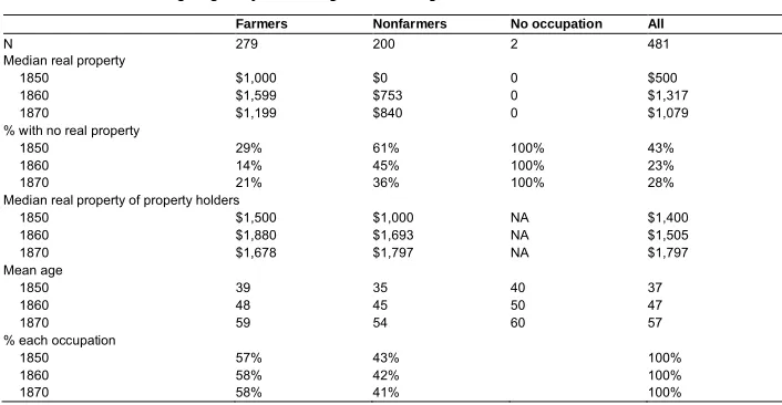
We began with the ‘full sample’ of 1,734 men in the genealogical dataset aged 20 or older who were located in the United States in the 1850 census. Since the spatial methods require a contiguous area with a minimal density of observations we could only analyze the ‘completer’ sample, a subset of 481 men found in each of the three censuses and who had remained within the geographic areas of New England, New York State, and northern Pennsylvania during those years. Attrition of the full 1850 sample was largely due to deaths, but also to men leaving the study area, usually for the Midwest, and to our inability to match individuals to both subsequent censuses. The full sample illustrates the opportunity that existed in the Midwest (Stewart 2006). By 1870 both farmers and nonfarmers in the Midwest were wealthier than men who stayed in the study region (see Table A-2, which compares the full and completer samples in detail).
Table 1: Real property of completer sample
Farmers Nonfarmers No occupation All
N 279 200 2 481
Median real property
1850 $1,000 $0 0 $500
1860 $1,599 $753 0 $1,317
1870 $1,199 $840 0 $1,079
% with no real property
1850 29% 61% 100% 43%
1860 14% 45% 100% 23%
1870 21% 36% 100% 28%
Median real property of property holders
1850 $1,500 $1,000 NA $1,400
1860 $1,880 $1,693 NA $1,505
1870 $1,678 $1,797 NA $1,797
Mean age
1850 39 35 40 37
1860 48 45 50 47
1870 59 54 60 57
% each occupation
1850 57% 43% 100%
1860 58% 42% 100%
1870 58% 41% 100%
Note: Missing occupations imputed from other censuses or the genealogy. Those with no occupation had no such information from any of these sources or they had equal numbers of farm and nonfarm occupational listings. Real property has been converted to 1850 dollars using conversion in Officer (2007).
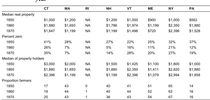
Between 1850 and 1870 there was no increase in the proportion of nonfarmers in our sample, even though the number of farms in southern New England decreased, probably because the cohort design does not allow us to study younger men just coming into the labor force. However, the completer sample does show the spatial differences in farming wealth in our county-level analysis. Usually wealth is strongly related to age as people accumulate property over time. But Table 2 shows that the median real property of farmers living in Massachusetts, New Hampshire, and Maine did not increase as expected due to the aging of the cohort between 1850 and 1870, while it did in New York, Vermont, Connecticut, and Pennsylvania.
Table 2: Real property of farmers in completer dataset by state and census year
CT MA RI NH VT ME NY PA
Median real property
1850 $1,000 $1,200 NA $1,200 $1,000 $900 $1,000 $562
1860 $1,880 $1,693 NA $1,786 $1,974 $1,199 $2,350 $1,880
1870 $1,647 $1,199 NA $1,199 $1,498 $720 $2,396 $1,528
Percent zero
1850 41% 28% NA 27% 22% 25% 32% 37%
1860 26% 7% NA 5% 16% 11% 21% 12%
1870 35% 7% NA 14% 28% 20% 27% 19%
Median of property holders
1850 $3,000 $2,000 NA $1,500 $1,425 $1,100 $1,800 $1,000
1860 $1,880 $1,693 NA $1,880 $2,350 $1,411 $2,820 $1,880
1870 $2,396 $1,199 NA $1,199 $2,396 $1,079 $2,994 $1,858
Proportion farmers
1850 17 43 0 40 41 51 65 14
1860 19 44 1 40 44 52 63 16
1870 20 43 1 36 43 54 67 16
5. Bayesian analysis
5.1 Spatial and family effects 5.1.1 Models
In order to analyze the longitudinal data presented in this project we have adopted a Bayesian hierarchical modeling paradigm. As we have repeated measures of the real wealth of individuals in our sample we can construct a longitudinal Bayesian model for the wealth dynamics. Bayesian models are characterized by hierarchical structures in parameters and are ideal for dealing with contextual and dynamic modeling issues (such as group characteristics, and changes with time). We assume that our outcome is
defined asyij wherei = 1,…,n denotes the individuals andj = 1,…,3 the time periods
(1850, 1860, 1870). We consider the general model in the form
yij :N(μij,κ–1) μij =xijtβ +v
i(iϵk) +ui(iϵk) +λj
Here the expected value of wealth is modeled as a function of a set of (possibly
random terms are spatial:vi(iϵk) +ui(iϵk), wherei th person is within thek th spatial unit,
and the temporal effect:λj.
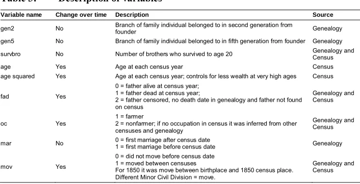
We tested two different types of models. In the first, the parameters were assumed constant for the three census years. In these, the data might have changed but the parameter for the variable was constant over time. For example, as time went on more men’s fathers died and this was included in the model. But the estimate for the effect of the father’s death was assumed to be the same at all three dates. However, whether or not the father had died could have affected wealth differently at each census date. Since men were leaving farming and so fewer men depended on inheriting land, it might have become less important over time. Therefore we also tested models in which the estimates for certain variables could vary over time. For the model with estimates that did not vary over time, we tested several different models. When we determined the model that fitted best, we then added the time-varying estimates to that model. The dependent variable was the log of real property at each census year, so we had 479 * 3 = 1,437 observations (two individuals whose occupations were missing were eliminated). We added a small positive constant ($2) to each real property value from the census so that we could log the real property. The spatial effects were modeled at the county level.
Table 3: Description of variables
Variable name Change over time Description Source
gen2 No Branch of family individual belonged to in second generation fromfounder Genealogy
gen5 No Branch of family individual belonged to in fifth generation from founder Genealogy
survbro No Number of brothers who survived to age 20 Genealogy andCensus
age Yes Age at each census year Census
age squared Yes Age at each census year; controls for less wealth at very high ages Census
fad Yes
0 = father alive at census year; 1 = father dead at census year;
2 = father censored, no death date in genealogy and father not found on census
Genealogy and Census
oc Yes 1 = farmer2 = nonfarmer; if no occupation in census it was inferred from other censuses and genealogy
Genealogy and Census
mar No 0 = first marriage after census date1 = first marriage before census date Genealogy
mov Yes
0 = did not move before census date 1 = moved between censuses
For 1850 it was move between birthplace and 1850 census place. Different Minor Civil Division = move.
Genealogy and Census
more recent family effects we did the same for the fifth generation, ‘gen5.’ 60% of the men in the completer sample were seven generations from the founder who came to America. Our analysis of father’s wealth captures more recent family effects.
Model 1: Covariate model with time as a factor. We used the variables above, adding a dummy variable for time: the three census dates.
Model 2: Model 1 plus two individual random effects: ‘ind1’ (a random effect for each individual) and ‘indT’ (a random effect for each individual at each census year).
Model 3: Model 2 plus two spatial effects: ‘region’ (a random effect for each county) and ‘region1’ (the correlated spatial effect, i.e., measuring the correlation of the spatial effects of adjoining counties). Because several counties’ boundaries changed over the study period due to growth and/or subdivision, we standardized all county boundaries to those in effect in 1850.
In addition to these three models, we tested other alternatives for each of the three models to see if we could improve the model fit:
(a) The basic covariate model above with time as a factor.
(b) MOV was replaced with the crow-flies distance of the moves from census to census. For 1850 we used the distance from the birthplace given in the genealogy to the place of enumeration in 1850. This was logged, and if zero was given a value of 1.
(c) Added real property per capita for the county where the individual was living (logged). The total real property of the county was divided by the population. In cases where the boundaries had changed, the population was redistributed back to the 1850 boundaries. The value of real property was distributed back on the basis of the area that had changed.
Improvements in model fit were measured by the Deviance Information Criterion (DIC) (Spiegelhalter et al. 2002). It is generally accepted that a reduction of the DIC by five to ten units represents a significant improvement in the fit of the model. This may occur even if the variables added to the model are not significant. In addition, the effective number of parameters in a model (pD) is also used as a secondary criterion for model parsimony.
5.1.2 Results
Table 4 displays the results of a variety of models fitted to these data. Of the three major models (1a, 2a, 3a) the best fit was for Model 2. The model fit was not improved by the addition of spatial effects (Model 3) or by the addition of the county per capita real property (Model 3c above), or by including only the county real property term and taking out the correlated spatial effect (Model 3d). Among the variants of Model 2, crow-flies distance moved (logged) did not improve the fit over a simple variable coding whether or not a move had occurred.
Table 4: Goodness of fit results for fitted models
Model Variables fitted DIC pD
1a Y ~ time+ age+age square + OC+ gen2+ gen5+ survbro+ fad+ mar+ mov 7,278.90 13.65
1b 1a - mov + log of distance 7,278.79 13.65
1c 1b + county level wealth variable 7,280.67 14.65
2a 1a + indRE+ timeRE 7,075.70 252.96
2b 1b + indRE+ timeRE 7,077.49 259.07
2c 1b + indRE+ timeRE + county level wealth variable 7,078.55 262.07
3a 1a + indRE+ timeRE + UH spatial effect +CH spatial effect 7,078.56 267.52
3b 1b + indRE+ timeRE + UH spatial effect +CH spatial effect 7,080.33 266.73
3c Y ~ time + county level wealth variable + age+ age square + OC+ gen2 + gen5 +survbro + fad+ mar+ log of distance + indRE+ timeRE + UH spatial effect +CH spatial effect
7,081.56 267.68
3d Y ~ time + county level wealth variable + age+ age square+ OC+ gen2 + gen5 +
+survbro+ fad+ log of distance+ mar+ indRE+ timeRE + UH spatial effect 7,078.18 264.00
Note: indRE: independent individual random effect; timeRE: independent time random effect; UH spatial effect: independent random effect of county; CH spatial effect: correlated random effect of county.
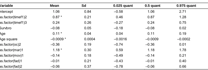
gen5 or gen2 (see Table 5: DIC = 7,064.85; pD = 247.14). This model had no spatial effects. It is possible that the reason we found no spatial effects was that they changed over time. To test for this we created a dummy variable (STINT = space time interaction) with unique values for each combination of county and time period. The addition of this variable to Model 2a did not improve the fit of the model.
Table 5: Estimates for model 2a without gen2 and gen5 without STINT Variable Mean Sd 0.025 quant 0.5 quant 0.975 quant
Intercept 1.06 0.84 –0.58 1.06 2.71
as.factor(timef1)2 0.87 * 0.21 0.46 0.87 1.28
as.factor(timef1)3 0.24 0.26 –0.27 0.24 0.75
Survbro –0.08 0.05 –0.18 –0.08 0.02
Age 0.11 * 0.04 0.04 0.11 0.19
Age square –0.0009 * 0.0004 –0.0016 –0.0009 –0.0002
as.factor(oc)2 –0.36 0.19 –0.74 –0.36 0.01
as.factor(mar)1 1.18 * 0.30 0.59 1.18 1.78
as.factor(mov)1 –0.14 0.18 –0.49 –0.14 0.21
as.factor(fad)1 –0.01 0.21 –0.43 –0.01 0.40
as.factor(fad)2 –0.06 0.37 –0.78 –0.06 0.66
Note: DIC = 7,064.85; pD = 247.14. Starred effects were statistically significant. 1850 Timef1= 1850; Timef2 = 1860; Timef3 =1870. In all other cases, the numbers next to each discrete variable are the value of that variable contrasted with 0.
In Model 2a, the best fitting model (Table 5), real property increased in 1860 over 1850 and this was significant. In 1870 it declined compared with 1850 (not significant). Age was significantly related to real property and age squared was negatively related. This is important because, as we saw in looking at the descriptive statistics, it could be difficult to distinguish cohort from temporal effects in our analysis. Here we have both in the analysis and they are both significant. The only other significant variable was marriage. Being married led to higher wealth. It was surprising that occupation had no significant effect, given what we have seen in the descriptive statistics. Actually, the estimates are very close to significance (if the .5 quantile is centered between the .025 and .972 quantiles this is truly not significant, but if the distribution around the .5 quantile is skewed it is closer to significance. The estimate of occupation is very skewed towards the negative, which means that nonfarmers had less wealth.) This is also true of the number of surviving brothers, where the negative sign means that the more brothers who survived to adulthood the less wealth a man would have.
fathers were censored, supporting the argument that many of the censored fathers were actually dead. The proportion married also increased with age/time. If moving were more likely in young adulthood and tapered off with age, as it does in contemporary data, then it too would be related to age. 39% of the completers moved between birth and 1850, 14% between 1850 and 1860, and 10% between 1860 and 1870. Although the first interval is longer than the decades between censuses, the slowing down could be due to the aging of the sample. Occupation also is related to age/time, since the younger men were more apt to be nonfarmers. Because of the collinearity we decided to drop the analysis with estimates that changed over time.
We have decided to mention a few results to show how such models are capable of distinguishing general temporal trends from the specific ways particular variables affect wealth over time. In the model with time-dependent estimates the effect of time itself was nearly identical to that in the model without time-dependent estimates. Thus, there was still a general significant effect of time in which men were wealthier in 1860 than in 1850 and wealth declined in 1870 (compared with 1850). There were also two significant time-dependent effects. First, occupation significantly decreased wealth in 1870; that is, being a nonfarmer led to significantly less wealth in 1870 compared with 1850. In 1860 the sign was positive; that is, farmers had more wealth. Moving between birth and 1850 led to increased wealth in 1850, but moving between 1850 and 1860 and between 1860 and 1870 decreased wealth, although it was only in 1860–1870 that this was statistically significant. Both of these effects may reflect the formation of a group of poor men in New England, men in the oldest settled areas who had left farming and moved to urban areas. These findings will be explored in more detail in a later section.
5.2 Wealth of fathers and sons
lessened over time, so that by 1870 the age of the sons was 52, while the average age of the fathers found in 1850 was 60. (The DIC was no different when the age difference between father and son was included, but because it is important to control for this, we report the estimates for this model.) The model is of the form:
yij:1+f timej +survbroi+ageij+ageij2+f occupi +f(mari)+f(movi)
+f fadi +log fareali +fasnadiffi,
wheref() denotes a factorial effect.
Table 6: Estimates for effect of the wealth of the father in 1850 on that of his son: Model 2a without gen2 and gen5 without STINT
Variable Mean Sd 0.025 quant 0.5 quant 0.975 quant
Intercept 4.22 * 1.62 1.04 4.22 7.41
as.factor(timef1)2 0.85 * 0.34 0.19 0.85 1.51
as.factor(timef1)3 0.03 0.47 –0.90 0.03 0.96
Survbro –0.06 0.08 –0.21 –0.06 0.09
Age –0.06 0.06 –0.18 –0.06 0.07
Age square 0.0012 0.0007 –0.0001 0.0012 0.0025
as.factor(oc)2 –0.12 0.27 –0.65 –0.12 0.41
as.factor(mar)2 1.52 * 0.38 0.77 1.52 2.27
as.factor(mov)1 –0.22 0.25 –0.72 –0.22 0.28
as.factor(fad)1 0.10 0.34 –0.57 0.10 0.77
as.factor(fad)2 –1.07 0.62 –2.28 –1.07 0.15
Logfareal50 –0.05 0.05 –0.14 –0.05 0.05
fasnadiff 0.003 0.023 –0.043 0.003 0.048
Note: DIC = 3,445.353; pD = 148.232. Starred variables are significant. See Table 5 for explanation of the other variables.
The DIC for a model without fareal or fasnadiff was 3,444.11, so adding these variables did not improve the model fit. The sign on the father’s wealth was negative and not significant, although it was somewhat skewed towards the negative. The age difference between the two was also not significant. Interestingly, the age effects were not significant in this analysis. This is quite unusual in the analysis of individual wealth. It seems that the effects of age in this younger group were entirely the effect of being married and whether or not one’s father was dead. Also, the time factor for 1870 had a much lower estimate than it did in the model that included all individuals. The 1870 decline was greater for this younger cohort and the 1860 peak more pronounced.
affected wealth. In order to model the interaction between coresidence and the wealth of the son we added an interaction term between being married and father’s wealth. We assigned the value of 2 to being married and 1 to being unmarried and multiplied that by the log of the father’s wealth. This would model the greater effect of father’s wealth on the wealth of married men. The effect of ‘logfareal’ was smaller and ‘mar’ was no longer significant, but neither was the interaction. Perhaps this younger cohort of completers was most affected by the changes in the economy, especially those between 1860 and 1870. Their wealth decreased during that time more than it had for the entire group of men. This would support the idea that during a time of transition the parents were unable to cushion the economic effect on their sons, at least those who remained in the region.
6. Moving and occupational changes
Both being a nonfarmer and moving prior to the census were associated with less wealth in 1870; in 1860 these effects existed but were not significant. Was a mobile underclass forming? We contrast three wealth groups, the top 10%, the bottom, and the rest. The thresholds for the top were $3,000 and above in 1850, $5,000 and above in 1860, and $8,000 and above in 1870. In order to avoid the effects of age on property ownership we defined the bottom as men between the ages of 35 and 60 with no real property, but the other categories included men of all ages. 11% were at the bottom in 1860 and this grew to 17% in 1870.
22% moved between 1860 and 1870 and 26% in the prior decade. Those at the bottom in 1860 were much more likely to have moved during both decades (1850 to 1860 = 39%; 1860 to 1870 = 36%). Moves were not as frequent in the top 10%: Wealthy nonfarmers in the study area did not move at all in the decade between 1860 and 1870. Those who did moved less far (median distance 9 miles) than the bottom (median 24 miles). The movers at the bottom in this decade did not usually go to cities.
7. Discussion
7.1 Spatial and temporal effects
There were significant temporal effects but no significant spatial effects, despite the evidence for changes in farm values in the study area during the period (also see spatial effects in the county-level analysis (Kasakoff et al. 2012)). Spatially sensitive measures of changes in wealth, such as the value of real property in each county at each date or a random effect for each county over time, did not improve model fit. In our analysis of individual wealth in 1860 using similar techniques, the random spatial effect at the county level improved model fit considerably. This effect might have represented counties where our families migrated early in the settlement process and got good land.
The absence of spatial effects in these models does not mean they did not exist. Nonfarmers were concentrated in southern New England where farms were declining in value, so occupation may mask spatial effects. Occupation was significant in our analysis of 1860, although not in the longitudinal analysis we present here. However, it was highly skewed in the direction of farmers being less wealthy. The real property of farmers declined in the oldest areas, and nonfarmers’ property holdings came to exceed those of farmers in 1870. It is also possible that the clustering of the families in the locations where they first settled has made it difficult to discern spatial effects that characterize the entire region. Also, spatial effects could exist at a smaller scale. When we plotted wealth among farmers on a soil map of one of the counties we found the wealthiest individuals lived in townships closest to rivers, probably due to the better soils there.
However, there was a significant temporal effect. There was a large and significant increase in real property between 1850 and 1860 and then a decrease from that point to a point only slightly above that of 1850, which was not statistically significant. This same effect was present in the analysis of the effect of the father’s wealth on that of his sons, even though that sample was much smaller and younger. The change in the source of grains from New York to the Midwest had already occurred and even before 1860 many farms in southern New England had lost value, yet real property held by these men increased. Because age was in the model, this is not due to the expected increase of wealth over the life course. The decline between 1860 and 1870 was not significant but, as we have seen, there are signs that a rural proletariat was developing.
nonfarmers too because of increased demand for goods, whether farm products or manufactured goods such as shoes, fabric for uniforms, and weaponry, all of which were produced in New England’s factories. By 1870 this part of the north had divided into two areas: those where farm values had declined (Massachusetts, Maine, and New Hampshire) and those where they stayed the same (New York, Pennsylvania, Connecticut, and Vermont) (see Table above and Wilson 1936). Vermont sent products to New York City via the Hudson River and new rail links and Connecticut was proximate to New York City. This suggests that it was the development of urban markets and transportation, not the war, which affected farmers the most.
One reason we do not see more of a decline between 1860 and 1870 may be that migrants from outside the United States, not included in our study, provided a safety net for native-born men by taking the least well-paying, nonfarming jobs. However, they lived largely in cities: In most of the largely rural counties where our sample lived, less than 10% of the population was foreign. The emergence of a mobile proletariat among older native-born men born during the period we are studying means that men in this group lost wealth despite the availability of foreign labor.
7.2 Family effects
The deep family effects that the genealogy allowed us to examine did not improve the model fit. This suggests that effects of earlier family decisions to move and pioneer (within the study area) were not lasting. (In the analysis for 1860 only gen2 improved the model fit. Maybe the peaking of farmers’ wealth at this date represented the last time when those decisions would have an effect on the group that remained in the area that had been settled the longest.) This study did not find evidence for Mare’s (2011) suggestion that inequality has deep roots in previous generations. However, a more recent decision to leave the study area for the Midwest did affect farmers’ wealth (see Table A-2). The only ‘family factor’ that proved to be significant was quite immediate: Marriage meant a man was more wealthy, which is not surprising given the long discussion in the literature of how when couples established new households in the West a certain amount of property was required for marriage (e.g., Engelen and Wolf 2005).
wealth of their fathers. Why then did we find in our study of 1860 that the wealth of brothers whose fathers were dead was correlated? We were unable to test for such an effect in the longitudinal analysis, but it is possible this effect would have disappeared by 1870 due to the increasing poverty of men who lived in certain parts of New England.
Another reason we did not find family effects in our longitudinal analysis may be that the 1860 analysis used the sum of real and personal property while the longitudinal analysis used only real property. In 1860, when personal property was first included in the census, slightly over half of the completers’ property was real estate. This proportion fell only slightly between 1860 and 1870, from 57% to 52%. Since more people had no real property in 1870 than in 1860 (22% in 1860 vs. 28% in 1870), this could have accounted for the decline. Farmers had a greater proportion of their total property in real estate than nonfarmers, as one would expect (65% in 1860 compared with 47% for nonfarmers in 1860). Extrapolating wealth on the basis of real property is more accurate for farmers than for nonfarmers.
It is difficult to study intergenerational effects on wealth using a cohort design. Because father’s wealth was from the census we could use only the younger men whose fathers were more apt to be alive. Father’s wealth was not significant and the sign was negative. In our analysis of 1860 it was significant, also with a negative sign, which we related to the coresidence of sons with their parents. Men still living at home usually had no wealth and had not married. This effect had outweighed the effect of those who had married and left home in 1860 in the subset with living fathers that we used – a younger group than the sample as a whole.
However, it is also possible that effects come and go quickly and affect certain cohorts more than others. 1860 may well have been the last moment the old family spatial hubs conferred advantage. The peak at this time for farmers may have been why our analysis for 1860 showed a significant effect of occupation but the longitudinal analysis did not.
8. Conclusions
the available sample. Most of the sons were still living at home. There were no significant differences in wealth between family branches in early generations.
These findings support Piketty’s observation that high rates of demographic increase and economic growth promote equality and economic mobility. Under these conditions, inheritance and family effects should be less important than in societies with lower rates of increase and economic growth, as existed in Europe at the time. Despite the spatial differences in wealth in both sectors in the region we are studying, the effect of growing up in a particular setting may not have been as important as it is in the United States today, when the population is growing much more slowly. Even though we did not find spatial or family effects in this analysis we would like to underscore the importance of methods of analysis that incorporate both. In order to tease out how families affect wealth, their effects need to be separated from the different economic characteristics of the places where family members reside.
Sjaastad (1962) wrote that economists should view migration as an investment whose benefits might be reaped by future generations, as Chetty et al. (2014) have demonstrated for a contemporary cohort in the United States. Our study of 1860 found family effects and spatial effects, which we hypothesized resulted from the timing of a family’s arrival in a particular community, but the longitudinal study we report in this article did not find such effects. Migration to the frontier paid off but eventually waned as the area developed and transportation and proximity to cities became more important for wealth. As research on the effect of previous generations on outcomes develops, models capable of distinguishing family effects from spatial proximity, such as those used here, will be necessary. However, temporal effects are important as well. We do not know how long intergenerational effects last. In our case, intergenerational effects may have been strongest at the 1860 peak and may have lessened thereafter. Thus, it will be important to also include temporal effects in such analyses.
9. Acknowledgements
References
Adams, J.W. and Kasakoff, A.B. (1984). Family and community in colonial New
England: The view from genealogies. Journal of Family History 9(1): 24–43.
doi:10.1177/036319908400900102.
Bowles, S., Gintis, S., and Groves, M.O. (eds.) (2008). Unequal chances: Family
background and economic success. Princeton: Princeton University Press. Chetty, R., Hendren, N., Kline, P., and Saez, E. (2014). Where is the land of
opportunity? The geography of intergenerational mobility in the United States. Quarterly Journal of Economics 129(4): 1553–1623.doi:10.3386/w19843.
Ditz, T.L. (1986).Property and kinship: Inheritance in early Connecticut, 1750–1820.
Princeton: Princeton University Press.doi:10.1515/9781400858293.
Engelen, T. and Wolf, A.P. (eds.) (2005). Marriage and the family in Eurasia:
Perspectives on the Hajnal hypothesis. Amsterdam: Askant.
Gates, P.W. (1965).Agriculture and the Civil War. New York: Knopf.
Gladwell, M. (2015, August 24). Starting over. The New Yorker: 32–37.
https://www.newyorker.com/magazine/2015/08/24/starting-over-dept-of-social-studies-malcolm-gladwell.
Jaremski, M. (2014). National Banking’s role in U.S. industrialization, 1850–1900. Journal of Economic History 74(1): 109–140. doi:10.1017/S0022050714000 047.
Kasakoff, A.B. (2010). Which sons lived closest to their elderly fathers? Sibling differences among native born families in the US North in 1850. In: Arrizabalaga, M-P., Bolovan, I., Eppel, M., Kok, J., and Nagata, M.L. (eds.). Many paths to happiness? Studies in population and family history. Amsterdam: Askant: 119–140.
Kasakoff, A.B., Lawson, A.B., Dasgupta, P., Feetham, S., and DuBois, M. (2013). Spatial inequality in wealth: A Bayesian analysis of the northeastern U.S. in
1860: Does space matter? Spatial Demography 1(1): 56–95. doi:10.1007/
BF03354887.
Kasakoff, A.B., Lawson, A.B., and Van Meter, E.M. (2014). A Bayesian analysis of the spatial concentration of individual wealth in the US North during the nineteenth
century.Demographic Research 30(36): 1035–1074.doi:10.4054/DemRes.2014.
Kearl, J.R. and Pope, C.L. (1984). Mobility and distribution.Review of Economics and Statistics 66(2): 192–199.doi:10.2307/1925819.
Kearl, J.R. and Pope, C.L. (1986a). Choices, rents and luck: Economic mobility of nineteenth-century Utah households. In: Engerman, S. and Gallman, R. (eds.). Long-term factors in American economic growth. Chicago: University of Chicago Press: 215–260.
Kearl, J.R. and Pope, C.L. (1986b). Unobservable family and individual contributions
to the distributions of income and wealth.Journal of Labor Economics 4(3, Part
2): S48–S79.doi:10.1086/298120.
Lindert, P.H. and Williamson, J.G. (2012). American incomes 1774–1860. Cambridge:
National Bureau of Economic Research (Working paper 18396). doi:10.3386/
w18396.
Mare, R.D. (2011). A multigenerational view of inequality.Demography 48(1): 1–23.
doi:10.1007/s13524-011-0014-7.
MetLife (2010). Inheritance and wealth transfer to baby boomers. Boston: Center for Retirement Research (A study by the Center for Retirement Research at Boston College for the MetLife Mature Market Institute).
Meyer, D.R. (2003).The roots of American industrialization. Baltimore: Johns Hopkins
University Press.
Officer, L.R. (2007). An improved long-run consumer price index for the United States. Historical Methods 40(3): 135–148.doi:10.3200/HMTS.40.3.135-148.
Piketty, T. (2014).Capital in the twenty-first century. Cambridge: Belknap.doi:10.415
9/9780674369542.
Pope, C. (2000). Inequality in the nineteenth century. In: Engerman, S.L. and Gallman,
R. (eds.). The Cambridge economic history of the United States, Vol. II.
Cambridge: Cambridge University Press: 109–142.doi:10.1017/CHOL9780521
553070.004.
Rosenberry, L.K.M. (1962). The expansion of New England: The spread of New
England settlement and institutions to the Mississippi River 1620–1865. New York: Russell.
Ruggles, S., Genadek, K., Goeken, R., Grover, J., and Sobek, M. (2015). Integrated public use microdata series: Version 6.0 [dataset]. Minneapolis: University of
Sjaastad, L.A. (1962). The costs and returns of human migration. Journal of Political Economy70(5, Part 2): 80–93.doi:10.1086/258726.
Solon, G. (1992). Intergenerational income mobility in the United States. American
Economic Review 82(3): 393–408.
Solon, G. (1999). Intergenerational mobility in the labor market. In: Ashenfelter, O.C.
and Card, D. (eds.).Handbook of labor economics. Amsterdam: Elsevier: 1761–
1800.doi:10.1016/S1573-4463(99)03010-2.
Solon, G. (2002). Cross-country differences in intergenerational earnings mobility. Journal of Economic Perspectives 16(3): 59–66.doi:10.1257/089533002760278 712.
Solon, G., Corcoran, M., Gordon, R., and Laren, D. (1991). A longitudinal analysis of
sibling correlations in economic status. Journal of Human Resources 26(3):
509–534.doi:10.2307/146023.
Spiegelhalter, D.J., Best, N.G., Carlin, B.P., and Van Der Linde, A. (2002). Bayesian
measures of model complexity and fit.Journal of the Royal Statistical Society,
Series B 64(4): 583–639.doi:10.1111/1467-9868.00353.
Steckel, R.H. and Moehling, C.M. (2001). Rising inequality: Trends in the distribution
of wealth in industrializing New England.Journal of Economic History 61(1):
160–183.doi:10.1017/S0022050701025086.
Stewart, J.I. (2006). Migration to the agricultural frontier and wealth accumulation,
1860–1870. Explorations in Economic History 43(4): 547–577. doi:10.1016/
j.eeh.2005.08.002.
Wilson, H.F. (1936).The hill country of northern New England.New York: Columbia
Appendix: Comparison of the ‘completer’ and ‘full’ samples
1. Attrition
The full sample consists of the 1,754 men aged 20 years or more in the families we are studying found in the 1850 census. However, we were only able to analyze 481 ‘completers,’ men who lived within the study area and were found in the census at all three dates. In what follows we discuss the difference between the completers and the larger sample. There was attrition from the full sample due to death, migration outside the study area (New England, the state of New York and some counties in northern Pennsylvania), and the inability to find men who were alive in all three censuses.
1.1 Death
Death is the major reason for attrition in our sample, accounting for the loss of at least 1,000 men. The genealogies provided death dates for 71% of the men we were tracing: 500 had died by 1870. 243 died between 1850 and 1860 (14%) and 257 between 1860 and 1870 (33% of those alive in 1860). Since this is a cohort that aged over time, a rising death rate is to be expected. From 1850 to 1860 there was no difference in the death rates within and outside the study area, but from 1860 to 1870 the death rate inside was higher (20%) than the rate outside (16%), reflecting the fact that the men outside were younger (by four years in 1860 and three in 1870).
1.2 Leaving the study area
Moving outside the study area was the second most important cause of attrition. Ohio
was settled in the first decade of the 19th century, the rest of the Midwest in the second.
1.3 Censorship
If the genealogy did not provide a death date and we did not find an individual in the census, we considered him censored. In all, censorship accounted for 591 cases of men not found at all three dates, several of whom were probably dead but whose deaths were unrecorded by the genealogist. The genealogists, most of whom lived in New England, did a less thorough job following men living outside the study area; also, perhaps, the records outside the study area were less complete. 74% of the men living inside the study area in 1850 had death dates in the genealogy, compared with 60% of the men living outside. In 1870 there was a bigger difference (71% v. 52%). 17% of the men who had lived within the study area were censored ten years later in 1860, compared with 25% of the men who had lived outside. The pattern continued with 22% of the men found inside the study area in 1860 censored ten years later, compared with 28% of the men who lived outside.
7% of the men found in 1850 were found in 1870 but not in 1860. This also varied by study area. We were less likely to find men (and to be able to link them to the genealogy) outside the study area than within it. Since the men within the study area were older, and many of the cases of censorship were actually deaths, the genealogists must have done a worse job following individuals, particularly younger men, in the Midwest than it seems from these statistics.
2. Wealth in the full sample
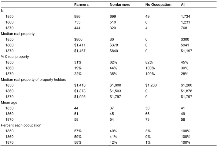
Overall, the wealth of the full sample increased over time (see Table A-1), which is not surprising because wealth is related to age. As one would expect, farmers had more real property than nonfarmers and there were fewer farmers with no real estate at all. When farmers and nonfarmers are combined there was an increase in real property between 1860 and 1870 – due, however, entirely to the men who had left farming. There was no increase in the median real property of farmers between 1860 and 1870, although the age of the men in the sample had increased by seven years. (The age difference from census to census is not ten years: Because of the deaths of older men, the sample gets younger over time.) The wealth of nonfarmers, on the other hand, increased dramatically, not only due to fewer men with no real property at all, but because men with property had more over time.
Table A-1: Real Property of Men age 20 or older in 1850 in the full sample Farmers Nonfarmers No Occupation All
N
1850 986 699 49 1,734
1860 735 510 6 1,231
1870 444 320 4 768
Median real property
1850 $800 $0 0 $300
1860 $1,411 $378 0 $941
1870 $1,467 $840 0 $1,197
% 0 real property
1850 31% 62% 82% 45%
1860 19% 44% 100% 30%
1870 22% 35% 100% 28%
Median real property of property holders
1850 $1,410 $1,000 $1,200 $1,200
1860 $1,878 $1,503 0 $1,878
1870 $1,995 $1,797 0 $1,797
Mean age
1850 44 37 50 41
1860 51 45 66 49
1870 58 54 73 56
Percent each occupation
1850 57% 40% 3% 100%
1860 59% 41% 0% 100%
1870 58% 42% 1% 100%
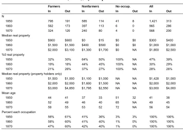
Table A-2: Wealth of men found in study area (‘In’) contrasted with men found outside the area (‘Out’), by occupation
Farmers Nonfarmers No occup. All
In Out In Out In Out In Out
N
1850 795 191 585 114 41 8 1,421 313
1860 562 173 397 113 6 0 965 286
1870 324 120 240 80 4 0 568 200
Median real property
1850 $900 $600 $0 $15 $0 $0 $300 $400
1860 $1,500 $1,500 $400 $500 $0 $0 $1,000 $1,000
1870 $2,000 $3,100 $1,300 $1,700 $0 NA $1,800 $2,500
%0 real property
1850 32% 30% 64% 50% 100% NA 47% 39%
1860 19% 18% 44% 45% 100% NA 30% 29%
1870 21% 26% 37% 27% 100% NA 28% 26%
Median real property (property holders only)
1850 $1,500 $1,000 $1,100 $1,000 NA NA $1,428 $1,000
1860 $2,000 $2,000 $1,600 $1,500 NA NA $2,000 $2,000
1870 $3,000 $4,850 $1,795 $2,550 NA NA $3,000 $4,000
Mean age
1850 44 41 37 33 51 32 41 38
1860 52 49 46 40 65 NA 49 45
1870 58 55 53 52 72 NA 56 54
Percent each occupation
1850 56% 61% 41% 36% 3% 3% 100% 100%
1860 58% 60% 41% 40% 1% 0% 100% 100%
1870 47% 60% 42% 40% 1% 0% 100% 100%