TOPSIS APPROACH TO CHANCE CONSTRAINED MULTI - OBJECTIVE MULTI- LEVEL QUADRATIC PROGRAMMING PROBLEM

(1)

[Pramanik et al., 3(6): June, 2016] ISSN 2349-4506

Impact Factor: 545

G

lobal

J

ournal of

E

ngineering

S

cience and

R

esearch

M

anagement

TOPSIS APPROACH TO CHANCE CONSTRAINED MULTI - OBJECTIVE MULTI-

LEVEL QUADRATIC PROGRAMMING PROBLEM

**Surapati Pramanik*, Durga Banerjee, B. C. Giri**

* Department of Mathematics, Nandalal Ghosh B.T. College, Panpur, P.O.-Narayanpur, District –North

24 Parganas, West Bengal, India-743126

Ranaghat Yusuf Institution, P. O. Ranaghat, Dist. Nadia, India-741201

Department of Mathematics, Jadavpur University, Jadavpur, West Bengal, India-700032

DOI:

10.5281/zenodo.55308

KEYWORDS

:

Multi – level programming, Multi – objective Decision Making, TOPSIS, Fuzzy Goal Programming, Chance Constraints.

ABSTRACT

This paper presents TOPSIS approach to solve chance constrained multi – objective multi – level quadratic programming problem. The proposed approach actually combines TOPSIS and fuzzy goal programming. In the TOPSIS approach, most appropriate alternative is to be finding out among all possible alternatives based on both the shortest distance from positive ideal solution (PIS) and furthest distance from the negative ideal solution (NIS). PIS and NIS for all objective functions of each level have been determined in the solution process. Distance functions which measure distances from PIS and NIS have been formulated for each level. The membership functions of the distance functions have been constructed and linearized in order to approximate nonlinear membership functions into equivalent linear membership functions. Stanojevic’s normalization technique for normalization has been employed in the proposed approach. For avoiding decision deadlock, each level decision maker provides relaxation on the upper and lower bounds of the decision variables. Two FGP models have been developed in the proposed approach. Euclidean distance function has been utilized to identify the optimal compromise solution. An illustrative example has been solved to demonstrate the proposed approach.

INTRODUCTION

Multilevel programming (MLP) is very useful technique to solve hierarchical decision making problem with multiple decision makers (DMs) in a hierarchical system. In MLP, each level DM independently controls some variables and tries to optimize his own objectives. For the successful running of a multilevel system, DMs try to find out a way/solution so that each level DM is satisfied at reasonable level. There are many approaches to solve MLP problem (MLPP) in the literature. Ananndalingam [1] proposed mathematical programming model of decentralized multi-level systems in crisp environment.

Lai [2] at first developed an effective fuzzy approach by using the concept of tolerance membership functions of fuzzy set theory [3] for solving MLPPs in 1996. Shih et al. [4] extended Lai’s concept by employing non-compensatory max-min aggregation operator for solving MLPPs. Shih and Lee [5] further extended Lai’s concept by introducing the compensatory fuzzy operator for obtaining satisfactory solution for MLPP. Sakawa et al. [6] developed interactive fuzzy programming to solve MLPP. Sinha [7, 8] further established an alternative fuzzy mathematical programming for MLPP. Pramanik and Roy [9] established fuzzy goal programming (FGP) approach to solve MLPP and presented sensitive analysis on relaxation provided by the upper level decision maker.. Linear plus linear fractional multilevel multi objective programming problem had been studied by Pramanik et al [10]. Han et al. [11] presented a case study on production inventory planning using reference based uncooperative multi follower tri level decision problem based on K – th best algorithm.

(2)

[Pramanik et al., 3(6): June, 2016] ISSN 2349-4506

Impact Factor: 545

G

lobal

J

ournal of

E

ngineering

S

cience and

R

esearch

M

anagement

Pramanik and Banerjee [17] developed chance constrained BLPP with quadratic objective functions. In their study [17] they converted chance constraints into deterministic constraints and solved the problem using FGP models. Pramanik et al. [18] studied linear plus linear fractional chance constrained BLPP. Pramanik et al. [19] also studied multilevel linear programming problem with chance constraints based on FGP.

TOPSIS stands for technique for order preference by similarity to ideal solution. In TOPSIS approach, most appropriate alternative is to be selected among all alternatives based on the shortest distance from positive ideal solution (PIS) and furthest distance from negative ideal solution (NIS). TOPSIS approach reduces multiple numbers of conflicting objectives to two objectives; one is the minimum of distance function which measures distance from PIS and another is the maximum of distance function which measures distance from NIS. Hwang and Yoon [20] introduced the TOPSIS approach to solve multi – attribute decision making problem. Lai et al. [21] established TOPSIS method for solving multi – objective decision making (MODM) problem. Chen [22] developed TOPSIS to solve multi criteria decision making. Jahanshahloo et al. [23] extended TOPSIS for decision making problem with fuzzy data. They used triangular fuzzy numbers for rating of each alternatives and weight of each criterion using  - cut method for normalization.

In neutrosophic environment Biswas et al. [24] proposed TOPSIS method for multi attribute decision making. In the evaluation process, Biswas et al. [24] employed linguistic variables to present the ratings of each alternative with respect to each attribute characterized by single-valued neutrosophic number. Biswas et al. [24] employed neutrosophic aggregation operator to aggregate all the opinions of decision makers. Dey et al. [25] studied generalized neutrosophic soft multi attribute group decision making based on TOPSIS. Pramanik et al. [26] established TOPSIS for single valued neutrosophic soft expert set based multi-attribute decision making problems. Dey et al. [27] studied TOPSIS for solving multi-attribute decision making problem under bi-polar neutrosophic environment.

Wang and Lee [28] developed fuzzy TOPSIS approach based on subjective weights and objective weights. Subjective weights are normalized into comparable scale. They adopted Shannon’s entropy [29] theory and defined closeness coefficient. Baky and Abo-Sinna [30] studied non-linear MODM problem using TOPSIS approach. Baky [31] developed interactive TOPSIS algorithms for solving multi – level non – linear multi – objective decision making problem. Dey et al. [32] studied TOPSIS approach to linear fractional MODM problem based on FGP. In their study they compared obtained results with Baky and Abo-Sinna’s [33] method and obtained better satisfactory results in terms of distance function.

In the present paper, we have presented TOPSIS approach to solve chance constrained multi-level multi objective quadratic programming problem. In the proposed approach, firstly, we have transformed chance constraints into equivalent deterministic constraints using known means and variances and confidence levels. PIS and NIS have been calculated for each objective function of each level. We have employed first order Taylor series for each nonlinear membership function to convert them into linear membership function. Then we have normalized them using Stanojevic’s normalization technique [34]. The above process has been done for each level and using FGP model to find optimal solution for each level separately. Each level DM provides his choice on the upper and lower bounds of the decision variables under his control. Two FGP models have been developed to get the optimal solution. Euclidean distance function has been used to find out the most appropriate optimal solution. The proposed TOPSIS method has been illustrated by solving a CCMLMOQPP.

(3)

[Pramanik et al., 3(6): June, 2016] ISSN 2349-4506

Impact Factor: 545

G

lobal

J

ournal of

E

ngineering

S

cience and

R

esearch

M

anagement

PROBLEM FORMULATION

Consider the following CCMLMOQPP.

1 x

MaxZ1 ( x ) =

1 x

MaxZ1 (x1,x2,...,xp)= 1

Max

x (Z11 ( x ), Z12 ( x ), ..., Z1 m1( x )) [FLDM] (1) 2

x

MaxZ2 ( x ) =

2 x

Max Z2 (x1,x2,...,xp) = 2

Max

x (Z21 ( x ), Z22 ( x ), ..., Z2m2( x )) [SLDM] (2)

. . .

p x

MaxZp( x ) =

p x

MaxZp(x1,x2,...,xp) = p x

Max(Zp1 ( x ), Zp2 ( x ), ...,

Z

pm_p( x )) [LLDM] (3)

Subject to

S

x = (

x



(

x

1

,

x

2

,...,

x

p

)



R

n: Pr (Ax _ 

B) I and x



0). (4)

Where

p s sp 3 s 2 s 1 s

p 2 23 22 21

p 1 13 12 11

a ... a a a

... ... ... ...

a ... a a a

a ... a a a A



    

 

    

 



1 s s 2 1

,

b

,...,

b

)

b

(

B



_

 ,

I are vectors of orders1and I is a vector having s numbers of 1, xi(xi1,xi2,...,xin_i),





(



1

,



2

,

...,



s

)

, i = 1, 2, …, p; n = n1+ n2 + …+ np

x d x 2 1 x c ) x (

Z t _ij

ij

ij   , (i = 1, 2, ..., p; j = 1, 2, ..., mi) (5)

Where c_ijis a vector of order 1n and dijis a vector of ordernn.

CONVERSION

OF

CHANCE

CONSTRAINTS

INTO

EQUIVALENT

DETERMINISTIC CONSTRAINTS

Consider the chance constraints of the form i i 1 p

1 j ij j

s ,..., 2 , 1 i ,

1 ) b x a

Pr(    



Using [17], the constraints can be written as follows:

1 i

i 1 i p

1 j ij j

s ,..., 2 , 1 i ) b var( ) ( ) b ( E x

a    

 

 (6)

Now, consider the chance constraints of the form

s ,..., 1 s i ,

1 ) b x a

Pr( i i 1

p

1 j ij j

  

   



Using [17], the constraint can be written as follows:

s ,..., 1 s i ,

) b var( ) ( ) b ( E x

a i i 1

1 i p

1 j ij j

  

  

 

 (7) 0

x ₍₈₎

where E(bi)and var(bi)are the expectation and variance of the random variable biand (.), (.) 1





(4)

[Pramanik et al., 3(6): June, 2016] ISSN 2349-4506

Impact Factor: 545

G

lobal

J

ournal of

E

ngineering

S

cience and

R

esearch

M

anagement

TOPSIS APPROACH

TOPSIS model for the FLDM

Consider the first level problem as

1 x

MaxZ1 ( x ) =

1 x

MaxZ1 (x1,x2,...,xp)= 1

Max

x (Z11 ( x ), Z12 ( x ), ...,Z1 m1( x )) [FLDM]

Subject to xS

Let 



_S 1j  1j

x Z (x) Z

Max and 



_S 1j  1j

x Z (x) Z

Min (j = 1, 2, …, m1) be the PIS and NIS for the FLDM. The distance

functions measuring the distances from the PIS and NIS can be defined as follows:

q / 1 1 m 1 j q j 1 j 1 j 1 j 1 q j ) 1 F ( PIS q ) Z Z ) x ( Z Z ( ) x ( d                  and q / 1 1 m 1 j q j 1 j 1 j 1 j 1 q j ) 1 F ( NIS q ) Z Z Z ) x ( Z ( ) x ( d                  (9) Thus the problem becomes

) x ( d Min PIS(F1)

q ) x ( d Max NIS(F1)

q

Subject to xS.

Construction of membership function for

d

(

x

q d * ) 1 F ( PIS x x ij ) 1 F ( PIS q d p 1 i 1 n 1 j * ) 1 F ( PIS ij ij * ) 1 F ( PIS ) 1 F ( PIS q d ) 1 F ( PIS q

d  

         

  (12)

Let Max (x) (xNIS(F1)*)

) 1 F ( NIS q d ) 1 F ( NIS q d S

x   and x (x ,x ,...,x )

* ) 1 F ( NIS p * ) 1 F ( NIS 2 * ) 1 F ( NIS 1 * ) 1 F ( NIS 

( _NIS₍_F₁₎

q d * ) 1 F ( NIS x x ij ) 1 F ( NIS q d p 1 i 1 n 1 j * ) 1 F ( NIS ij ij * ) 1 F ( NIS ) 1 F ( NIS q d ) 1 F ( NIS q

d  

         

(5)

[Pramanik et al., 3(6): June, 2016] ISSN 2349-4506

Impact Factor: 545

G

lobal

J

ournal of

E

ngineering

S

cience and

R

esearch

M

anagement

Stanojevic’s normalization technique

Adopting Stanojevic’s normalization technique [34], the linear membership functions can be normalized as follows:

) 1 F ( PIS ) 1 F ( PIS

) 1 F ( PIS )

1 F ( PIS q d )

1 F ( PIS q

d _b _a

a ) x ( ˆ ) x (

  



 wherea Minˆ _PIS₍_F₁₎(x)

q d S x ) 1 F (

PIS  



 b Maxˆ PIS(F1)(x) q d S x ) 1 F (

PIS  



 (14)

) 1 F ( NIS ) 1 F ( NIS

) 1 F ( NIS )

1 F ( NIS q d )

1 F ( NIS q

d _b _a

a ) x ( ˆ ) x (

  



 wherea Minˆ _NIS₍_F₁₎(x)

q d S x ) 1 F (

NIS  



 b Maxˆ NIS(F1)(x) q d S x ) 1 F (

NIS  



 (15)

FGP model to obtain satisfactory solution for FLDM

Using the FGP model of Pramanik and Banerjee [17] in order to obtain the satisfactory solution for the FLDM, the FGP model appears as:

S x

1 Min

 

 (16)

, 1 d

) x

( PIS(F1) )

1 F ( PIS q

d  

 

, 1 d

) x

( NIS(F1) )

1 F ( NIS q

d  

 

, 1 d

0

, 1 d

0

, d

) 1 F ( NIS

) 1 F ( PIS

) 1 F ( NIS 1

) 1 F ( PIS 1

 

 

   

Subject to xS

Solving the above model, the satisfactory solution for the FLDM has been obtained as )

x ..., , x , x (

x F1*

p * 1 F 2 * 1 F 1 * 1

F 

TOPSIS model for the SLDM

Let 



 2j  2j S

x Z (x) Z

Max and 



_S 2j  2j

x Z (x) Z

Min (j = 1, 2, …, m2) be the PIS and NIS for the SLDM. The distance

functions measuring the distances from the PIS and NIS can be defined as

q / 1 2

m

1 j

q

j 2 j 2

j 2 j 2 q j )

2 F ( PIS

q )

Z Z

) x ( Z Z ( )

x ( d

    

   

   

  



and

q / 1 2

m

1 j

q

j 2 j 2

j 2 j

2 q j )

2 F ( NIS

q )

Z Z

Z ) x ( Z ( )

x ( d

    

   

  



  



(17) Thus the problem becomes

) x ( d Min PISq (F2)

) x ( d Max NIS(F2)

q

Subject to xS

d

(

x

),

d

NIS(F2)

(

x

)

q ) 2 F ( PIS q

Let 



 d (x)(d (x))

Min PIS(F2) q )

2 F ( PIS q S

x and

 

 d (x)(d (x))

Max PIS(F2) q )

2 F ( PIS q S x

d

PIS(F2)

(

x

)

(6)

[Pramanik et al., 3(6): June, 2016] ISSN 2349-4506

Impact Factor: 545

G

lobal

J

ournal of

E

ngineering

S

cience and

R

esearch

M

anagement

) x ( d )) x ( d ( 1 )) x ( d ( ) x ( d )) x ( d ( )) x ( d ( )) x ( d ( ) x ( d )) x ( d ( ) x ( d )) x ( d ( , 0 ) x ( ) 2 F ( PIS q ) 2 F ( PIS q ) 2 F ( PIS q ) 2 F ( PIS q ) 2 F ( PIS q ) 2 F ( PIS q ) 2 F ( PIS q ) 2 F ( PIS q ) 2 F ( PIS q ) 2 F ( PIS q ) 2 F ( PIS q ) 2 F ( PIS q d                (18)

Let 



 d (x)(d (x))

Min NIS(F2) q ) 2 F ( NIS q S x and  

 d (x)(d (x))

Max NIS(F2) q ) 2 F ( NIS q S x

d

NIS(F2)

(

x

)

) x ( d )) x ( d ( 1 )) x ( d ( ) x ( d )) x ( d ( )) x ( d ( )) x ( d ( )) x ( d ( ) x ( d )) x ( d ( ) x ( d , 0 ) x ( ) 2 F ( NIS q ) 2 F ( NIS q ) 2 F ( NIS q ) 2 F ( NIS q ) 2 F ( NIS q ) 2 F ( NIS q ) 2 F ( NIS q ) 2 F ( NIS q ) 2 F ( NIS q ) 2 F ( NIS | q ) 2 F ( NIS q ) 2 F ( NIS q d                (19)

Let Max (x) (xPIS(F2)*)

) 2 F ( PIS q d ) 2 F ( PIS q d S

x   and x (x ,x ,...,x )

* ) 2 F ( PIS p * ) 2 F ( PIS 2 * ) 2 F ( PIS 1 * ) 2 F ( PIS 

( _PIS₍_F₂₎

q d * ) 2 F ( PIS x x ij ) 2 F ( PIS q d p 1 i 2 n 1 j * ) 2 F ( PIS ij ij * ) 2 F ( PIS ) 2 F ( PIS q d ) 2 F ( PIS q

d  

        

  (20)

Let Max (x) (xNIS(F2)*)

) 2 F ( NIS q d ) 2 F ( NIS q d S

x   and x (x ,x ,...,x )

* ) 2 F ( NIS p * ) 2 F ( NIS 2 * ) 2 F ( NIS 1 * ) 2 F ( NIS 

( NIS(F2)

q d * ) 2 F ( NIS x x ij ) 2 F ( NIS q d p 1 i 2 n 1 j * ) 2 F ( NIS ij ij * ) 2 F ( NIS ) 2 F ( NIS q d ) 2 F ( NIS q

d  

         

  (21)

Stanojevic normalization technique

Adopting Stanojevic’s normalization technique [34] the linear membership functions have been normalized as follows: ) 2 F ( PIS ) 2 F ( PIS ) 2 F ( PIS ) 2 F ( PIS q d ) 2 F ( PIS q

d _b _a

a ) x ( ˆ ) x (    

 wherea Minˆ _PIS₍_F₂₎(x)

q d S x ) 2 F (

PIS  



 ,b Maxˆ PIS(F2)(x) q d S x ) 2 F (

PIS  

  (22) ) 2 F ( NIS ) 2 F ( NIS ) 2 F ( NIS ) 2 F ( NIS q d ) 2 F ( NIS q

d _b _a

a ) x ( ˆ ) x (    

 wherea Minˆ _NIS₍_F₂₎(x)

q d S x ) 2 F (

NIS  



 ,b Maxˆ NIS(F2)(x) q d S x ) 2 F (

NIS  



 (23)

FGP model to obtain satisfactory solution for SLDM

Using the model of Pramanik and Banerjee [17] in order to obtain the satisfactory solution for the SLDM, the FGP model can be written as:

S x 2 Min

 

 (24)

1 d

) x

( PIS(F2) ) 2 F ( PIS q

d  

  , , 1 d ) x

( NIS(F2) ) 2 F ( NIS q

d  

 

, d_PIS₍_F₂₎ 2     

2 dNIS(F2), , 1 d

(7)

[Pramanik et al., 3(6): June, 2016] ISSN 2349-4506

Impact Factor: 545

G

lobal

J

ournal of

E

ngineering

S

cience and

R

esearch

M

anagement

, 1 d

0 _NIS ₍_F₂₎

Solving the above model, the obtained satisfactory solution for the SLDM has been denoted by ) x ..., , x , x (

x F2*

p * 2 F 2 * 2 F 1 * 2

F  _.

TOPSIS model for the LLDM

Let 



_S pj  pj

x Z (x) Z

Max and 



 pj  pj S

x Z (x) Z

Min (j = 1, 2, …, mp) be the PIS and NIS for the LLDM. The distance

functions measuring the distances from the PIS and NIS can be defined as follows:

q / 1 p m 1 j q pj pj pj pj q j ) Fp ( PIS q ) Z Z ) x ( Z Z ( ) x ( d                  and q / 1 p m 1 j q pj pj pj pj q j ) Fp ( NIS q ) Z Z Z ) x ( Z ( ) x ( d                  (25) Thus the problem becomes

) x ( d Min PIS(Fp)

q ) x ( d Max NIS_q (Fp) Subject to xS

d

(

x

q d * ) Fp ( PIS x x ij ) Fp ( PIS q d p 1 i np 1 j * ) Fp ( PIS ij ij * ) Fp ( PIS ) Fp ( PIS q d ) Fp ( PIS q

d  

         

  (28)

Let Max (x) (xNIS(Fp)*)

) Fp ( NIS q d ) Fp ( NIS q d S

x   and x (x ,x ,...,x )

* ) Fp ( NIS p * ) Fp ( NIS 2 * ) Fp ( NIS 1 * ) Fp ( NIS 

(8)

[Pramanik et al., 3(6): June, 2016] ISSN 2349-4506

Impact Factor: 545

G

lobal

J

ournal of

E

ngineering

S

cience and

R

esearch

M

anagement

) x ( ˆ )

x ) x ( (

) x x ( ) x ( )

x

( _NIS₍_Fp₎

q d * ) Fp ( NIS x x ij

) Fp ( NIS q d p

1 i

p n

1 j

* ) Fp ( NIS ij ij *

) Fp ( NIS ) Fp ( NIS q d ) Fp ( NIS q

d  

 

 

 

 



  (29)

Stanojevic’s normalization technique

Adopting Stanojevic’s normalization technique [34] the linear membership functions can be normalized as follows:

) Fp ( PIS ) Fp ( PIS

) Fp ( PIS )

Fp ( PIS q d )

Fp ( PIS q

d _b _a

a ) x ( ˆ ) x (

  



 wherea Min ˆ _PIS₍_Fp₎(x)

q d S x ) Fp (

PIS  



 ,b Maxˆ PIS(Fp)(x) q d S x ) Fp (

PIS  



 (30)

) Fp ( NIS ) Fp ( NIS

) Fp ( NIS )

Fp ( NIS q d )

Fp ( NIS q

d _b _a

a ) x ( ˆ ) x (

  

 

wherea Minˆ _NIS₍_Fp₎(x)

q d S x ) Fp (

NIS  



 ,b Maxˆ NIS(Fp)(x) q d S x ) Fp (

NIS  



 (31)

FGP model to obtain satisfactory solution for LLDM

Using the model of Pramanik and Banerjee [17] in order to obtain the satisfactory solution for the LLDM, the FGP model can be written as:

S x

p Min

 



(32)

, 1 d

) x

( PIS(Fp) )

p ( PIS q

d  

 

, 1 d

) x

( NIS(Fp) )

Fp ( NIS q

d  

 

, 1 d

0 ; 1 d

0

, d ; d

) Fp ( NIS )

Fp ( PIS

) Fp ( NIS p ) Fp ( PIS p

 

  



 

Solving the above model, the obtained satisfactory solution for the SLDM has been denoted by )

x ..., , x , x (

x Fp*

p * Fp 2 * Fp 1 * Fp 

SELECTION OF PREFERENCE BOUNDS

In the multi – level decision making problem, the goals of all levels are generally conflicting. To execute the decision making in the real situation, cooperation between DMs is needed. For the overall satisfaction, each level DM provides some relaxation on their decision variables. So, the i-th level provides the upper and lower bounds on the decision variable xi. Let tLi(Fi)and

) Fi ( R i

t be the lower and upper bounds on the decision variables (i = 1, 2, …, p). Then the bounds can be written as follows:

) Fi ( R i * Fi i i ) Fi ( L i * Fi

i t x x t

x     (33) Wherexi(xi1,xi2,...,xin_i),x (x ,x ,...,x )

* Fi

i in * Fi

2 i * Fi

1 i * Fi

i  ,

t

(

t

,

t

,...,

t

)

) Fi ( L

i in ) Fi ( L

2 i ) Fi ( L

1 i ) Fi ( L

i



,

t

(

t

,

t

,...,

t

)

) Fi ( R

i in ) Fi ( R

2 i ) Fi ( R

1 i ) Fi ( R i



FGP MODELS

Using FGP model of Pramanik and Banerjee [17], the two FGP models have been presented as follows:

Model – 1

Min  (34) Subject to

, 1 d

) x

( _PIS₍_Fi₎ )

Fi ( PIS q

d  

(9)

[Pramanik et al., 3(6): June, 2016] ISSN 2349-4506

Impact Factor: 545

G

lobal

J

ournal of

E

ngineering

S

cience and

R

esearch

M

anagement

,

1 d

) x

( NIS(Fi) )

Fi ( NIS q

d  

 

, 1 d

0

, 1 d

0

, d

) Fi ( NIS

) Fi ( PIS

) Fi ( NIS ) Fi ( PIS

 

 

   

p ..., , 2 , 1 i for , t x x t

x_iFi* _iL(Fi) _i _iFi* R_i(Fi) 

S x . Model – 2

) 35 ( )

d w d

w (

Min NIS(Fi) NIS i p

1

i PIS(Fi) PIS i

 

 _ 

 

, 1 d

) x ( to subject

) Fi ( PIS )

Fi ( PIS q

d  

 

, 1 d

) x

( NIS(Fi) )

Fi ( NIS q

d  

 

, 1 d

0

, 1 d

0

) Fi ( NIS

) Fi ( PIS

 

 

, 1 ) w w

( NISi p

1 i

PIS

i  

 

p ..., , 2 , 1 i for , t x x t

x R(Fi)

i * Fi i i ) Fi ( L i * Fi

i     

S x .

SELECTION OF OPTIMAL SOLUTION

Zeleny’s distance function [35] can be defined as follows:

r / 1 r K

1

k k

r k

r( ,K) [ (1 ) ]

L    

 (36)

Here, _kmeans attribute level and K 1

1

k k

 

 r(0r)denotes the distance parameter and krepresents the

degree of closeness between compromise solution and individual best solution of the k – th objective function. In this paper, we consider r = 2, then distance function becomes K 2 1/2

1

k k

2 k

2( ,K) [ (1 ) ]

L    

 (37)

For the maximization problem, _kis the ratio of the compromise solution and individual best solution of the k – th objective function. For the minimization type, the ratio would be reversed. Minimum L₂reflects the best optimal compromise solution.

NUMERICAL EXAMPLE

Consider the following numerical example to illustrate the proposed approach. ]

FLDM [ ) x x x z ); 4 x ( ) 3 x )( 2 x ( z (

max 3

2 2 2 1 12 3 2

1 11 1 x

       

] SLDM [ ) x x x z ; x x x ( z (

max ₂₁ ₁ ₂ ₃ ₂₂ ₁ ₂ ₃ 2

x

  



] LLDM [ ) x x 3 x 2 z ); 5 x )( 1 x ( ) 7 x ( z (

max 2 3

2 1 32 3 1 2

31 3 x

      

Subject to

1 1

3 2

1 x x b ) 1

x (

(10)

[Pramanik et al., 3(6): June, 2016] ISSN 2349-4506

Impact Factor: 545

G

lobal

J

ournal of

E

ngineering

S

cience and

R

esearch

M

anagement

2 2

3 2

1 5x 3x b ) 1

x 2 (

Pr       ,

3 3

3 2

1 4x 2x b ) 1

x 3 (

Pr      , x1 0, x2  0, x3  0.

The means, variances and the confidence levels are given below: E(b1) = 3, var(b1) = 2, 1 = 0.03

E(b2) = 12, var(b2) =8, 2= 0.01

E(b3) =10, var(b3) = 18, 3= 0.05

Using (6), (7) the chance constraints involved in the proposed problem have been transformed into equivalent deterministic constraints as:

666 . 5 x x

x1 2 3 ,

576 . 18 x 3 x 5 x

2 1 2 3

 ,

021 . 3 x 2 x 4 x

3 1 2 3 , First level MODM problem

] FLDM [ ) x x x z ); 4 x ( ) 3 x )( 2 x ( z (

max 3

2 2 2 1 12 3 2

1 11 1 x

       

Subject to

666 . 5 x x

x1 2 3 ,

576 . 18 x 3 x 5 x

2 1 2 3

 ,

021 . 3 x 2 x 4 x

3 1 2 3 ,

x1 0, x2  0, x3  0.

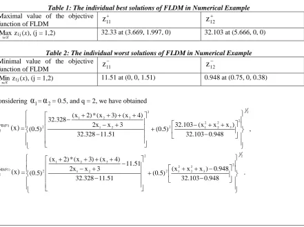
The individual best solutions (PISs) and the individual worst solutions (NISs) of the objective functions considered by the FLDM subject to the constraints have been respectively shown in the Table 1 and Table 2.

Table 1: The individual best solutions of FLDM in Numerical Example

Maximal value of the objective function of FLDM



11

z

₁₂

S x

Max



 z1j (x), (j = 1,2) 32.33 at (3.669, 1.997, 0) 32.103 at (5.666, 0, 0)

Table 2: The individual worst solutions of FLDM in Numerical Example

Minimal value of the objective function of FLDM



11

z

₁₂

S x

Min



 z1j (x), (j = 1,2) 11.51 at (0, 0, 1.51) 0.948 at (0.75, 0, 0.38)

Considering

α

₁=

α

₂= 0.5, and q = 2, we have obtained

) x ( dPIS(F!)

2 = ,

948 . 0 103 . 32

) x x x ( 103 . 32 ) 5 . 0 ( 51

. 11 328 . 32

3 x 2x

) 4 x ( ) 3 x ( * ) 2 x ( 328 . 32 ) 5 . 0 (

2 1

2 3 2 2 2 1 2

2

2 1

3 2

1

2

      

      

   

 

    

   

 

   

 

  

   



) x ( dNIS(F1)

2 =

2 1

2 3

2 2 2 1 2 2

2 1

3 2

1

2

948 . 0 103 . 32

948 . 0 ) x x x ( ) 5 . 0 ( 51

. 11 328 . 32

51 . 11 3

x 2x

) 4 x ( ) 3 x ( * ) 2 x ( ) 5 . 0 (

      

      

   

 

    

   

 

   

 



 



   

(11)

[Pramanik et al., 3(6): June, 2016] ISSN 2349-4506

Impact Factor: 545

G

lobal

J

ournal of

E

ngineering

S

cience and

R

esearch

Min

+(x3 –

0) ) 0 , 0 , 666 . 5 ( x at 3 NIS(F1) 2 d x ) x (            

=ˆ NIS(F1)(x)

2 d



= 1 + 3.3128((x1 – 5.666)



0.4696 + (x2 – 0)



0.2734+ (x3 – 0)0.0677),

Normalizing ˆ PIS(F1)(x)

2 d

 andˆ NIS(F1)(x)

2 d

 , we have obtained the following,

) x ( PIS(F1) 2 d

 = _PIS(F1) _PIS(F1)

PIS(F1) PIS(F1) 2 d a b a ) x ( ˆ   

, where

b

PIS(F1)=

S

Max

 x ) x ( ˆ _PIS(F1) 2 d

 = 0.999 and

a

PIS(F1)=

S

Min

 x ) x ( ˆ _PIS(F1) 2 d

 = -0.431;

) x ( NIS(F1) 2 d

 = _NIS(F1) _NIS(F1)

NIS(F1) NIS(F1) 2 d a b a ) x ( ˆ   

, where

b

NIS(F1)=

S

Max



x (x)

ˆ _NIS(F1)

2 d

 = 1 and

a

NIS(F1)=

S

Min



x (x)

ˆ _NIS(F1)

2 d

 = -7.476. Solve the model (16) in order to get the satisfactory solution of FLDM:

(12)

[Pramanik et al., 3(6): June, 2016] ISSN 2349-4506

Impact Factor: 545

G

lobal

J

ournal of

E

ngineering

S

cience and

R

esearch

M

anagement

, 1 d

) x

( NIS(F₁) )

1 F ( NIS q

d  

 

, 1 d

0

, 1 d

0

,. d

, d

) 1 F ( NIS

) 1 F ( PIS

) 1 F ( NIS 1

) 1 F ( PIS 1

 

 

   

666 . 5 x x

x1 2 3 ,

576 . 18 x 3 x 5 x

2 1 2 3

 ,

021 . 3 x 2 x 4 x

3 1 2 3 ,

x1 0, x2  0, x3  0.

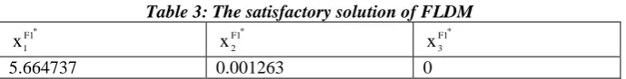
The satisfactory solution of FLDM has been provided in the Table 3.

Table 3: The satisfactory solution of FLDM

* F1 1

x F1*

2

x F1*

3

x

5.664737 0.001263 0

Suppose that the FLDM decides x1F1*= 5.66 with upper tolerance R(F1) 1

t = 0.34 and lower tolerance L(F1) 1

t = 3.66 such that 5.66 – 3.66



x1



5.66 + 0.34.

8.2 Second level MODM problem

] SLDM [ ) x x x z ; x x x ( z (

max ₂₁ ₁ ₂ ₃ ₂₂ ₁ ₂ ₃

2 x

  



Subject to

666 . 5 x x

x1 2 3 ,

576 . 18 x 3 x 5 x

2 1 2 3

 ,

021 . 3 x 2 x 4 x

3 1 2 3 ,

x1 0, x2  0, x3  0.

,he individual best solutions (PISs) and the individual worst solutions (NISs) of the objective functions considered by the SLDM subject to the constraints have been respectively shown in the Table 4 and Table 5.

Table 4: The individual best solutions of SLDM in Numerical Example

Maximal value of the objective function of SLDM



2 1

z z_{2 2}

S x

Max



 z2j (x), (j = 1,2) 5.941871 at (0.26, 1.43, 3.98) 7.326 at (3.67, 1.997, 0)

Table 5: The individual worst solutions of SLDM in Numerical Example

Minimal value of the objective function of SLDM



2 1

z z2 2

S x

Min_

 z2j (x), (j = 1,2) 0 at (0, 0, 1.51) 0 at (1.007, 0, 0)

Considering

α

₁=

α

₂= 0.5, and q = 2, we have obtained

) x ( dPIS(F2)

2 = ,

0 326 . 7

) x x x ( 326 . 7 ) 5 . 0 ( 0

942 . 5

) x x x ( 942 . 5 ) 5 . 0 (

2 1 2 3 2 1 2

2 3 2 1 2

    

  

  



   

  



  

) x ( dNIS(F2)

2 =

2 1 2 3 2 1 2 2 3 2 1 2

0 326 . 7

0 ) x x x ( ) 5 . 0 ( 0 942 . 5

0 x x x ) 5 . 0 (

    

  

   

 

   

  



  

(13)

[Pramanik et al., 3(6): June, 2016] ISSN 2349-4506

Impact Factor: 545

G

lobal

J

ournal of

E

ngineering

S

cience and

R

esearch

M

anagement

Now,



d

PIS(F2)

(

x

)





2 =

S

Min



x

PIS(F2) 2

d (x) = 0.129 at (2.59, 1.817, 1.259);



d

PIS(F2)

(

x

)





2 =

S

Max



x

PIS(F2) 2

d (x) = 0.6499 at (1.007,0, 0);



d

NIS(F2)

(

x

)





2 =

S

Max



x

NIS(F2) 2

d (x) = 0.5877 at (3.669, 1.997, 0);



d

NIS(F2)

(

x

)





2 =

S

Min



x

NIS(F2) 2

d (x) = 0.065 at (0.6, 0, 0.609).

The membership functions of PIS(F2) 2

d (x) and NIS(F2) 2

, 129

. 0 ) x ( d if 1,

6499 . 0 ) x ( d 129 . 0 if , 129 . 0 6499 . 0

) x ( d 6499 . 0

) x ( d 0.6499 if 0,

) x (

PIS(F2) 2

PIS(F2) 2 PIS(F2)

2

PIS(F2) 2

PIS(F2) 2 d

      



 

 



 

) x (

NIS(F2) 2 d

 =





      



 





5877 . 0 ) x ( d if 1,

5877 . 0 ) x ( d 065 . 0 if , 065 . 0 5877 . 0

065 . 0 -) x ( d

065 . 0 ) x ( d if 0,

NIS(F2) 2

NIS(F2) 2 NIS(F2)

2

NIS(F2) 2

2 d

 and NIS(F2)(x)

2 d

 can be transformed into equivalent linear membership functionsˆ PIS(F2)(x)

2 d

) x (

PIS(F2) 2 d





~ ˆ PIS(F2)(x)

2 d



= 1 + (x1 – 2.59)0.2835+ (x2 – 1.817)0.3854 + (x3 – 1.259)0.2980

) x (

NIS(F2) 2 d





~ ˆ NIS(F2)(x)

2 d



= 1 + (x1 – 0.6) (-0.1245) + (x2 – 0) (-0.1257) + (x3 – 0.609)(-0.083),

Normalizing ˆ PIS(F2)(x)

2 d

 , we have obtained

) x (

PIS(F2) 2 d

 = _PIS(F2) _PIS(F2)

PIS(F2) PIS(F2)

2 d

a b

a ) x ( ˆ

  

, where

b

) x ( Min

) 2 F ( PIS )

2 F ( PIS q d

2

 

 



, 1 d

) x

( NIS(F2) )

2 F ( NIS q

d  

 





2 dPIS(F2),





2 dNIS(F2), 1 d

0 _PIS ₍_F₂₎  , 1 d

0 _NIS ₍_F₂₎  ,

666 . 5 x x

x1 2 3 ,

576 . 18 x 3 x 5 x

2 1 2 3

 ,

021 . 3 x 2 x 4 x

3 1 2 3 ,

x1 0, x2  0, x3  0.

(14)

[Pramanik et al., 3(6): June, 2016] ISSN 2349-4506

Impact Factor: 545

G

lobal

J

ournal of

E

ngineering

S

cience and

R

esearch

M

anagement

Table 6: The satisfactory solution of SLDM

* F2 1

x F2*

2

x F2*

3

x

3.669308 1.996692 0

Assume that the SLDM decides xF22*= 1.997 with upper tolerance R(F2) 2

t = 0.003 and lower tolerance L(F2) 2

t =1.997 such that 1.997 – 1.997



x2



1.997 + 0.003.

Last level MODM problem

] LLDM [ ) x x 3 x 2 z ); 5 x )( 1 x ( ) 7 x ( z (

max 2 3

2 1 32 3 1 2

31 3 x

      

Subject to

666 . 5 x x

x1 2 3 ,

576 . 18 x 3 x 5 x

2 1 2 3

 ,

021 . 3 x 2 x 4 x

3 1 2 3 ,

x1 0, x2  0, x3  0.

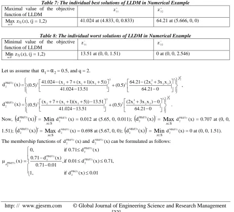
The individual best solutions (PISs) and the individual worst solutions (NISs) of the objective functions of the LLDM subject to the constraints have been respectively shown in the Table 7 and Table 8.

Table 7: The individual best solutions of LLDM in Numerical Example

Maximal value of the objective function of LLDM



3 1

z z3 2

S x

Max



 z3j (x), (j = 1,2) 41.024 at (4.833, 0, 0.833) 64.21 at (5.666, 0, 0)

Table 8: The individual worst solutions of LLDM in Numerical Example

Minimal value of the objective function of LLDM



3 1

z z3 2

S x

Min_

 z3j (x), (j = 1,2) 13.51 at (0, 0, 1.51) 0 at (0, 0, 2.546)

Let us assume that

α

₁=

α

₂= 0.5, and q = 2.

) x ( dPIS(F3)

2 = ,

0 21 . 64

) x x 3 x 2 ( 21 . 64 ) 5 . 0 ( 51

. 13 024 . 41

)) 5 x )( 1 x ( 7 x ( 024 . 41 ) 5 . 0 (

2 1 2 3 2 2 1 2

2 3 1 2

2

    

  

   

 

   

  





    

) x ( dNIS(F3)

2 =

2 1 2 3 2 2 1 2 2 3

1 2

2

0 21 . 64

0 ) x x 3 x 2 ( ) 5 . 0 ( 51

. 13 024 . 41

51 . 13 )) 5 x )( 1 x ( 7 x ( ) 5 . 0 (

    

  

   

 

  

   



     

.

Now,



d

PIS(F3)

(

x

)





2 =

S

Min



x

PIS(F3) 2

d (x) = 0.012 at (5.65, 0, 0.011);



d

PIS(F3)

(

x

)





2 =

S

Max



x

PIS(F3) 2

d (x) = 0.707 at (0, 0, 1.51);



d

NIS(F3)

(

x

)





2 =

S

Max



x

NIS(F3) 2

d (x) = 0.698 at (5.67, 0, 0);



d

NIS(F3)

(

x

)





2 =

S

Min



x

NIS(F3) 2

d (x) = 0 at (0, 0, 1.51). The membership functions of PIS(F3)

2

d (x) and NIS(F3) 2

, 01 . 0 ) x ( d if 1,

71 . 0 ) x ( d 01 . 0 if , 01 . 0 71 . 0

) x ( d 71 . 0

) x ( d 71 0. if 0,

) x (

PIS(3) 2

PIS(F3) 2 PIS(F3)

2

PIS(F3) 2

PIS(F3) 2 d

      

  

 



(15)

[Pramanik et al., 3(6): June, 2016] ISSN 2349-4506

Impact Factor: 545

G

lobal

J

ournal of

E

ngineering

S

cience and

R

esearch

M

anagement

) x (

NIS(F3) 2 d

 =

      

  





698 . 0 ) x ( d if 1,

698 . 0 ) x ( d 0 if , 0 698 . 0

0 -) x ( d

0 ) x ( d if 0,

NIS(F3) 2

NIS(F3) 2 NIS(F3)

2

NIS(F3) 2

2 d

 and NIS(F3)(x)

2 d

 can be transformed into equivalent linear membership functionsˆ PIS(F3)(x)

2 d

) x (

PIS(F3) 2 d





~ ˆ PIS(F3)(x)

2 d



= 1 +0.0093((x1 – 5.65)0.00333+ (x2 – 0)*0.00309 + (x3 – 0.01)0.00047)

) x (

NIS(F3) 2 d





~ ˆ NIS(F3)(x)

2 d



= 1 + 1.02474((x1 – 5.67) 0.72871 + (x2 – 0) 0.18832+ (x3 – 0)0.48636),

Now, Normalize ˆ PIS(F3)(x)

2 d

 we get the following,

) x (

PIS(F3) 2 d

 = _PIS(F3) _PIS(F3)

PIS(F3) PIS(F3)

2 d

a b

a ) x ( ˆ

  

, where PIS(F3)

b

3

Min 

, 1 d

) x

( PIS(F3) )

3 F ( PIS q

d  

 

, 1 d

) x

( _NIS₍_F₃₎ )

3 F ( NIS q

d  

 

, 1 d

0

, 1 d

0

, d

) 3 F ( NIS

) 3 F ( PIS

) 3 F ( NIS 3

) 3 F ( PIS 3

 

 

   

666 . 5 x x

x1 2 3 ,

576 . 18 x 3 x 5 x

2 1 2 3

 ,

021 . 3 x 2 x 4 x

3 1 2 3 ,

x1 0, x2  0, x3  0.

The satisfactory solution of LLDM has been provided in the Table 9.

Table 9: The satisfactory solution of FLDM

* F3 1

x F3*

2

x F3*

3

x

5.666 0 0

Assume that the LLDM decides F3* 3

x = 0 with upper tolerance R(F3) 3

t = 1 and lower tolerance L(F3) 3

t =0 such that 0-0



x3



0 + 1.

(16)

[Pramanik et al., 3(6): June, 2016] ISSN 2349-4506

Impact Factor: 545

G

lobal

J

ournal of

E

ngineering

S

cience and

R

esearch

M

anagement

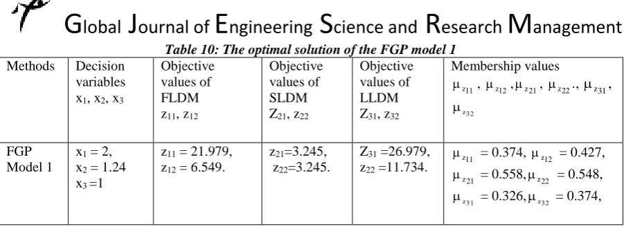
Table 10: The optimal solution of the FGP model 1

Methods Decision variables x1, x2, x3

Objective values of FLDM z11, z12

Objective values of SLDM Z21, z22

Objective values of LLDM Z31, z32

Membership values 11

z

 , 12 z

 ,

21 z

 , .,

22 z

 ,

31 z



3 2 z



FGP Model 1

x1 = 2,

x2 = 1.24

x3 =1

z11 = 21.979,

z12 = 6.549.

z21=3.245,

z22=3.245.

Z31 =26.979,

z22 =11.734.

11 z

 = 0.374, 12 z

 = 0.427, 21

z

 = 0.558, 22 z

 = 0.548,

3 1 z

 = 0.326,

3 2 z

 = 0.374,

The optimal solution of the FGP Model 2 is shown in the Table 11.

Table 11: The optimal solution of the FGP model 2

Methods Decision variables x1, x2, x3

Objective values of FLDM z11, z12

Objective values of SLDM Z21, z22

Objective values of LLDM Z31, z32

Membership values 11

z

 , 12 z

 ,

21 z

 , z₂₂., z31,

3 2 z



FGP Model 2

x1 = 2,

x2 = 1.24

x3 =1

z11 = 21.979,

z12 = 6.549.

z21=3.245,

z22=3.245.

Z31 =26.979,

z22 =11.734.

11 z

 = 0.374, 12 z

 = 0.427, 21

z

 = 0.558, 22 z

 = 0.548,

3 1 z

 = 0.326,

3 2 z

 = 0.374,

Note1. Two tables show the two FGP Models provide the same results

CONCLUSION

In the paper we have developed TOPSIS approach to solve chance constrained multi-level multi objective quadratic programming problem. In the proposed approach two FGP models have been developed and solved. Further, the proposed approach can be extended to solve multi-level multi objective quadratic programming problem with fuzzy coefficient of objective functions. If the coefficients of constraints are taken as random variables, the proposed concept can also be adopted.

REFERENCES

1. Anandalingam, G. (1988). A mathematical programming model of decentralized multi-level systems, Journal of the Operational Research Society 39 (11), 1021-1033.

2. Lai, Y. J. (1996). Hierarchical optimization: a satisfactory solution, Fuzzy Sets and Systems 77 (3), 321– 335.

3. Zadeh

4. Shih, H. S., Lai, Y. J., Lee, E. S. (1996). Fuzzy approach for multi-level programming problems, Computers & Operations Research 23 (1), 73-91.

5. Shih, H. S., Lee, E. S. (2000). Compensatory fuzzy multiple level decision making, Fuzzy Sets and Systems 114 (1), 71-87.

6. Sakawa, M., Nishizaki, I., Uemura, Y. (1998). Interactive fuzzy programming for multilevel linear programming problems, Computers and Mathematics with Applications 36 (2), 71-86.

7. Sinha, S. (2003). Fuzzy mathematical programming applied to multi-level programming problems, Computers and Operations Research 30(9), 1259 – 1268.

8. Sinha, S. (2003). Fuzzy programming approach to multi-level programming problems, Fuzzy Sets and Systems 136(2), 189 – 202.

(17)

[Pramanik et al., 3(6): June, 2016] ISSN 2349-4506

Impact Factor: 545

G

lobal

J

ournal of

E

ngineering

S

cience and

R

esearch

M

anagement

10. Pramanik, S., Banerjee, D., Giri, B. C. (2015). Multi-level multi-objective linear plus linear fractional programming problem based on FGP approach, International Journal of Innovative Science Engineering and Technology 2 (6), 153-160.

11. Han, J., Lu, J., Hu, Y., Zhang, G. (2015). Tri-level decision-making with multiple followers: model, algorithm and case study, Information Sciences 311, 182–204.

12. Pramanik, S. (2012). Bilevel programming problem with fuzzy parameter: a fuzzy goal programming approach, Journal of Applied Quantitative Methods 7(1), 09-24.

13. Pramanik, S., Dey, P.P. (2011). Bi-level multi-objective programming problem with fuzzy parameters, International Journal of Computer Applications 30 (10), 13-20.

14. Pramanik, S., Dey, P.P, Giri, B.C. (2011). Decentralized bilevel multiobjective programming problem with fuzzy parameters based on fuzzy goal programming, Bulletin of Calcutta Mathematical Society. 103 (5), 381—390.

15. Pramanik, S. (2015). Multilevel programming problems with fuzzy parameters: a fuzzy goal programming approach, International Journal of Computer Applications 122 (21), 34-41.

16. Sakawa, M., Nishizaki, I., Uemura, Y. (2000). Interactive fuzzy programming for multi-level linear programming problems with fuzzy parameters, Fuzzy Sets and Systems 109 (1), 03 – 19.

17. Pramanik, S., Banerjee, D. (2012). Chance constrained quadratic bilevel programming problem, International Journal of Modern Engineering Research 2(4), 2417-2424.

18. Pramanik, S., Banerjee, D., Giri, B.C. (2012). Chance Constrained Linear Plus Linear Fractional Bi-level Programming Problem, International Journal of Computer Applications 56(16), 34-39.

19. Pramanik, S., Banerjee, D., Giri, B.C. (2015). Chance constrained multi-level linear programming problem, International Journal of Computer Applications 120 (18), 01-06.

20. Hwang, C. L., Yoon, K. (1981). Multiple attribute decision making: Methods and applications, Springer-Verlag, Helderberg.

21. Lai, Y. J., Liu, T. J., Hwang, C. J. (1994). TOPSIS for MODM, European Journal of Operational Research 76 (3), 486-500.

22. Chen, C. T. (2000). Extensions of the TOPSIS for group decision-making under fuzzy environment, Fuzzy Sets and Systems 114 (1), 1–9.

23. Jahanshahloo, G. R., Hosseinzadeh L. F., Izadikhah, M. (2006). Extension of the TOPSIS method for decision – making problems with fuzzy data, Applied Mathematics and Computation 181, 1544 - 1551. 24. Biswas, P., Pramanik, S., Giri, B.C. (2015). TOPSIS method for multi-attribute group decision making under single-valued neutrosophic environment, Neural Computing and Applications. DOI: 10.1007/s00521-015-1891-2.

25. Dey, P.P., Pramanik, S. Giri, B.C. (2015). Generalized neutrosophic soft multi-attribute group decision making based on TOPSIS, Critical Review 11, 41- 55.

26. Dey, P.P., Pramanik, S., Giri, B.C. (2015).TOPSIS for single valued neutrosophic soft expert set based multi-attribute decision making problems, Neutrosophic Sets and Systems 10, 88- 95.

27. Dey, P.P., Pramanik, S., Giri, B.C. (2016). TOPSIS for solving multi-attribute decision making problems under bi-polar neutrosophic environment, In Smarandache, F. & Pramanik, S.(Eds) “New Trends in Neutrosophic Theories and Applications", Bruxelles: EuropaNova. In Press.

28. Wang, T. C., Lee, H. (2009). Developing a fuzzy TOPSIS approach based on subjective weights and objective weights, Experts Systems with Applications 36, 8980 – 8985.

29. Shannon, C. E., Weaver, W. (1947). The mathematical theory of communication, Urbana: The University of Illinois Press.

30. Abo-Sinna, M. A., Amer, A. H., Ibrahim, A. S. (2008). Extensions of TOPSIS for large scale multi-objective non-linear programming problems with block angular structure, Applied Mathematical Modelling 32 (3), 292–302.

31. Baky, I. A. (2014). Interactive TOPSIS algorithms for solving multi-level non - linear multi – objective decision – making problems, Applied Mathematical Modelling 38, 1417-1433.

32. Dey, P. P., Pramanik, S., Giri, B. C. (2014). TOPSIS approach to linear fractional bi-level MODM problem based on fuzzy goal programming, Journal of Industrial Engineering International 10, 173–184. 33. Baky, I. A. and Abo-Sinna, M. A. (2013). TOPSIS for bi-level MODM problems, Applied Mathematical

(18)

[Pramanik et al., 3(6): June, 2016] ISSN 2349-4506

Impact Factor: 545

G

lobal

J

ournal of

E

ngineering

S

cience and

R

esearch

M

anagement

34. Stanojević, B. (2013). A note on Taylor series approach to fuzzy multiple objective linear fractional programming, Information Sciences 243, 95-99.