The Thirty-Third AAAI Conference on Artificial Intelligence (AAAI-19)
Weighted Oblique Decision Trees
∗Bin-Bin Yang, Song-Qing Shen, Wei Gao
National Key Laboratory for Novel Software TechnologyNanjing University, Nanjing, 210023, China {yangbb, shensq, gaow}@lamda.nju.edu.cn
Abstract
Decision trees have attracted much attention during the past decades. Previous decision trees include axis-parallel and oblique decision trees; both of them try to find the best splits via exhaustive search or heuristic algorithms in each iteration. Oblique decision trees generally simplify tree structure and take better performance, but are always accompanied with higher computation, as well as the initialization with the best axis-parallel splits. This work presents the Weighted Oblique Decision Tree (WODT) based on continuous optimization with random initialization. We consider different weights of each instance for child nodes at all internal nodes, and then obtain a split by optimizing the continuous and differentiable objective function of weighted information entropy. Extensive experiments show the effectiveness of the proposed algorithm.
Introduction
Decision trees have attracted much attention in many real applications such as computer vision (Bosch, Zisserman, and Munoz 2007) and information retrieval (Fuhr and Pfeifer 1994). The classical decision trees include CART (Breiman et al. 1984), ID3 (Quinlan 1986), C4.5 (Quin-lan 1993), etc. This motivates a series of studies (Murthy, Kasif, and Salzberg 1994; Loh and Shih 1997; Breiman 2001; Geurts, Ernst, and Wehenkel 2006; Shotton et al. 2013b; Fan 2016; Abuzaid et al. 2016; Zhou and Feng 2017). Recent years have witnessed an increasing popularity on decision trees, for example, Microsoft Kinect makes real time human pose estimation from single depth images by decision trees trained on millions of examples (Shotton et al. 2013a).
The basic idea of decision trees is to seperate data with some certain splitting criterion, recursively. This procedure requires an optimization at each internal node of the tree, which partitions the training data in the node into subsets according to some splitting criteria, such as information gain (Quinlan 1993) or Gini impurity index (Breiman et al. 1984). A large number of decision trees have been developed to exploit univariate split functions, according to the feature value below some threshold or not. We call it axis-parallel decision tree since the split at each node can be viewed as
∗
Supported by the National Key R&D Program of China (2017YFB1001903), NSFC(61751306, 61876078).
Copyright c2019, Association for the Advancement of Artificial Intelligence (www.aaai.org). All rights reserved.
an axis-parallel hyperplane in the feature space, and these trees have made successful applications (Cicalese, Laber, and Saettler 2014; Shotton et al. 2013a).
The axis-parallel decision trees may yield complex tree structure and increase computational cost, when decision boundaries are not parallel to axes. Hence, an oblique split is introduced to make a multivariate linear combina-tion of features followed by binary quantizacombina-tion. Generally, oblique decision trees simplify tree structure and achieve better performance (Breiman et al. 1984; Heath, Kasif, and Salzberg 1993; Brodley and Utgoff 1995; Loh and Shih 1997; Amasyali and Ersoy 2008; Robertson, Price, and Reale 2013; Kontschieder et al. 2015). While training oblique decision trees is always followed with high running-time cost, as well as the initialization with best axis-parallel splits (Murthy, Kasif, and Salzberg 1994; Norouzi et al. 2015).
This work introduces another oblique decision tree based on continuous optimization with random initialization. The main contributions can be summarized as follows:
• Motivated from weighted information entropy, we consider different weights of each instance for child nodes at all internal nodes, and then obtain a split by optimizing a continuous and differentiable objective function. Here we introduce the ‘soft’ splitting instead of ‘hard’ splitting to tackle the intractability for continuous optimization. Our method proceeds with random initialization, whereas previous oblique decision trees require initialization with the best axis-parallel splits.
• Extensive experiments show that our method simplifies tree structure, and achieves significantly better perfor-mance than state-of-the-art algorithms of decision trees. Our experiments also show that previous oblique decision trees can not obtain small-size trees without the best axis-parallel splitting initialization. Moreover, our method takes relatively less running-time cost, especially for datasets of dimensionality larger than200, such asusps,proteinand
mnist. We finally analyze the tree depths of the proposed WODT method.
Relevant Work
Decision trees have a long history from the early work (Mes-senger and Mandell 1972), which employed a measure of node impurity based on the distribution of class labels for each internal node. Quinlan (1993) and Breiman et al. (1984) introduced the famous C4.5 and CART decision trees based on entropy and Gini index, respectively. Loh and Shih (1997) presented a two-step QUEST tree by spliting each node with significance tests. Due to simplicity and interpretabil-ity, a large number of axis-parallel decision trees have been developed in the literature (Domingos and Hulten 2000; Zhou and Chen 2002; Geurts, Ernst, and Wehenkel 2006; Shotton et al. 2013a; Abuzaid et al. 2016), and decision trees have been used as base learners for ensemble algorithms such as boosting and bagging (Breiman 2001; Friedman 2001; Zhou 2012).
Oblique decision trees present another way to construct compact trees and achieve better performance, and the main difference lies in the splits of multivariate linear combinations over features. CART (Breiman et al. 1984) can be applied to oblique decision tree by optimizing the coefficients of oblique splits based on the coordinate descent method. Murthy, Kasif, and Salzberg (1994) made a refinement of CART to find a local optimum by multiple restarts and random perturba-tions. Some statistical techniques are suggested for oblique decision trees, such as least square method and linear discrim-inant analysis (Brodley and Utgoff 1995; Loh and Shih 1997; Bennett and Blue 2002; L´opez-Chau et al. 2013).
There are also some heuristic oblique decision trees with good performance under proper assumptions (Amasyali and Ersoy 2008; Manwani and Sastry 2012). In addition, various models have been developed by combining neural networks with decision trees, but with complex structure and high computational cost (Str¨omberg, Zrida, and Isaksson 1991; Guo and Gelfand 1992; Setiono and Liu 1999; Kontschieder et al. 2015). Norouzi et al. (2015) proposed the oblique de-cision tree by optimizing a continuous loss, which upper bounds the empirical 0/1 loss with the-best-axis-parallel-split initialization. Our method utilizes the robust sigmoid function to obtain a continuous and differentiable objective function, and proceeds with random initialization.
Preliminaries
LetX ⊂RdandY ={1,2, ..., C}denote the instance and
label space, respectively. Suppose thatDis an (unknown) underlying distribution over the product spaceX × Y. Let
Sm ={(x1, y1),(x2, y2), ...,(xm, ym)}be a training data,
where each example is drawn i.i.d. from the distributionD. An oblique decision tree is generally constructed as fol-lows. An instancex∈ Xis directed from the root of the tree down through internal nodes to a leaf node. Each leaf node specifies a distribution over the label spaceY, and each inter-nal node performs a binary test by evaluating a split function
sθ(x) :Rd→R. Ifsθ(x)<0, thenxis directed to the left
child node; and the right child otherwise. Here,sθ(x) =θTx
is parameterized byθ∈Rd, and we further incorporate an
offset parameter to obtain split functions of the formθTx+b
by appending a constant ”+1” to the feature vector.
For each internal node, we aim to find a parameterθfor a good oblique split. However, it is difficult to make direct continuous optimization w.r.t.θ, since the indicator function
I[sθ(x)<0]is a discontinuous and piecewise-constant
func-tion (Breiman et al. 1984; Murthy, Kasif, and Salzberg 1994; Norouzi et al. 2015). Here,I[·]denotes the indicator function, which returns 1 if the argument is true and 0 otherwise.
Our WODT Method
Motivated from weighted information entropy (Guias¸u 1971), this section introduces another oblique decision tree based on instance weights. The basic idea is to consider different weights of each instance for child nodes when searching for split parameters, and obtain a good oblique split by optimiz-ing a continuous and differentiable objective function. We use the ‘soft’ splitting instead of ‘hard’ splitting to tackle the intractability for gradient-based optimization.
At an internal node, letSbe the set of training examples in this node. Without loss of generality, we assume
S ={(x1, y1),(x2, y2), ...,(xn, yn)} for n≤m.
Given split parameterθ, we compute the weight w.r.t. the left child node by selecting sigmoid function over the negative of the split functionsθ(x), i.e.,
σ(−sθ(x)) =σ(−θTx) = 1/(1 +eθ
Tx ),
and the weight w.r.t. right child node is given by
1−σ(−sθ(x)) = 1−σ(−θTx) =σ(θTx).
LetSLandSRdenote the set of training examples and the
corresponding weights w.r.t. the left and right child nodes, respectively, i.e.,
SL={((xi, yi), wiL)|w L
i =σ(−θ Tx
i),(xi, yi)∈S}, SR={((xi, yi), wiR)|w
R i =σ(θ
Tx
i),(xi, yi)∈S}.
LetWLandWR be the sum of weights w.r.t. the left and
right child nodes, respectively, that is,
WL(θ) =
X
((xi,yi),wiL)∈SL
wiL,
WR(θ) =
X
((xi,yi),wiR)∈SR
wRi .
We further denote byWk
LandWRk the sum of weights in left
and right child nodes w.r.t. each classk∈ Y, respectively, by
WLk(θ) = X
((xi,yi),wLi)∈SL
I[yi=k]wLi,
WRk(θ) = X
((xi,yi),wRi)∈SR
I[yi=k]wRi .
We finally have the objective functionE(θ)as
E(θ) =WL(θ)HL(θ) +WR(θ)HR(θ),
whereHLandHRare the left and right weighted information
entropies, respectively. More precisely, we have
HL(θ) =− C
X
k=1
Wk L(θ) WL(θ)
log2W
k L(θ) WL(θ) ,
HR(θ) =− C
X
k=1
Wk R(θ) WR(θ)
log2W
Algorithm 1InduceSubtree(S, D, d)of Weighted Oblique Decision Tree (WODT)
Input: Training dataS, maximum tree depthD, depth of the current noded
1: Create a nodepbased on dataS
2: if Examples in dataSall belong to classk∈ Ythen 3: Nodepis a leaf node labelled with classk
4: end if
5: if d > D then
6: Nodepis a leaf node labelled with the majority class
k0∈ Y 7: end if
8: Calculate the split parameterθby the L-BFGS algorithm according to Eqns. (1) and (2)
9: Obtain the training data for the left-child and right-child nodes according to Eqns.(3) and (4), respectively. 10: The left subtree of nodep: InduceSubtree(L, D, d+ 1) 11: The right subtree of nodep: InduceSubtree(R, D, d+ 1) Output: A decision subtree with the root nodep
The objective functionE(θ)can be further expressed as
E(θ) =WLlog2WL+WRlog2WR
−
C
X
k=1
WLklog2WLk−
C
X
k=1
WRklog2WRk. (1)
It is easy to observe that the objective functionE(θ)is continuous and differentiable w.r.t. the split parameterθ, and we could make use of standard optimization techniques to find a good split parameterθ, such as gradient-descent and quasi-Newton method. It is important to calculate the gradient functiong(θ)of our objective functionE(θ), that is,
g(θ) =dE(θ)/dθ.
We have
g(θ)·ln 2 = (1 + lnWL) dWL
dθ + (1 + lnWR) dWR
dθ
−
C
X
k=1
(1 + lnWLk)dW
k L
dθ −
C
X
k=1
(1 + lnWRk)dW
k R dθ .
Fromσ(−z) = 1−σ(z),σ0(z) =σ(z)(1−σ(z)), we have
dWL
dθ =
n
X
i=1
σ(−θTxi)[1−σ(−θTxi)](−xi)
=−
n
X
i=1
[1−σ(θTxi)]σ(θTxi)xi=− dWR
dθ .
For simplicity, we denote by
βi=σ(θTxi)[1−σ(θTxi)]xi,
and we have dWR/dθ = Pni=1βi. Similarly, we have dWLk/dθ =−dWRk/dθanddWRk/dθ =Pn
i=1I[yi=k]βi.
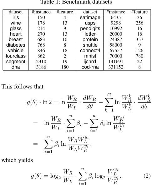
Table 1: Benchmark datasets
dataset #instance #feature dataset #instance #feature
iris 150 4 satimage 6435 36
wine 178 13 usps 9298 256
glass 214 9 pendigits 10992 16
heart 270 13 letter 20000 16
breast 683 10 protein 24387 357
diabetes 768 8 shuttle 58000 9
vehicle 846 18 connect4 67557 126
fourclass 862 2 mnist 70000 780
segment 2310 19 ijcnn1 141691 22
dna 3186 180 cod-rna 331152 8
This follows that
g(θ)·ln 2 = lnWR
WL
· dWR
dθ −
C
X
k=1 lnW
k R Wk L
· dW
k R dθ
= lnWR
WL
·
n
X
i=1
βi− n
X
i=1
βiln Wyi
R Wyi
L
=
n
X
i=1
βiln
WRW
yi
L WLWRyi
,
which yields
g(θ) = log2WR
WL
·
n
X
i=1
βilog2
Wyi
L Wyi
R
. (2)
In the implementation, we can use vectorization methods to accelerate our WOTD method according to Eqns. (1) and (2). We also optimize the objective functionE(θ)based on the L-BFGS algorithm, where we initialize the parameterθ
with random vectors. This is quite different from previous oblique decision trees which require the initialization with the best axis-parallel splits. The parameterθis not initialized to the zero vector so as to avoid the zero gradient.
Given the split parameterθ, we partition data as follows:
L = {(x, y)∈S|θTx<0}, (3)
R = {(x, y)∈S|θTx≥0}. (4)
As can be seen, we make use of the direction of split param-eterθto partition data, while the objective functionE(θ)is related with norm and direction of parameterθ simultane-ously. A natural idea is to make an additional constraint over the norm of θand then utilize the projection or Lagrange multiplier as in the work (Norouzi et al. 2015). Here, we do not make any additional constrain sinceσ(θTx)will be ap-proximated by floating-point numbers in the implementation of the proposed method.
Algorithm 1 presents the detailed description of the weighted oblique decision subtree. Given an instancex∈ X and weighted oblique decision tree of Algirhtm 1, we predict the label of instancexaccording to the leaf node at the end of the path traversed by instancex.
Experiments
Table 2: Comparison of test accuracies (mean±std.) on benchmark datasets.•/◦indicates that WODT is significantly better/worse than the corresponding method (pairwiset-tests at95%significance level). ‘N/A’ means that no results were obtained after running out 250000 seconds (about 3 days).
dataset our WODT APDT CO2 CO2r OC1 OC1r CART-LC CART-LCr
iris .9733±.0248 .9467±.0499• .9467±.0540• .9263±.0526• .9600±.0442 .9400±.0554• .9467±.0499• .9000±.1125• wine .9665±.0323 .9271±.0529• .9271±.0579• .8818±.0565• .9213±.0456• .8876±.1293• .9494±.0450 .9045±.0529• glass .6216±.0256 .6521±.1215 .6521±.0517◦ .5837±.0740• .6168±.1056 .6075±.0810 .7056±.0763◦ .6215±.1142
heart .7630±.0429 .7370±.0737 .7370±.0300• .7167±.0446• .7593±.0668 .7815±.0898 .6815±.1285• .7556±.0529
breast .9590±.0099 .9466±.0581 .9346±.0458• .9378±.0190• .9341±.0608• .9356±.0639• .9414±.0271• .9517±.0173• diabetes .7161±.0191 .7090±.0486 .6908±.0370• .6953±.0306• .6667±.0387• .6914±.0541• .7161±.0335 .6784±.0379• vehicle .7069±.0383 .7045±.1603 .7223±.0466 .6501±.0180• .6418±.1568• .6927±.1050 .6702±.1212 .7069±.0402
fourclass .9896±.0043 .9843±.0164 .9809±.0191• .8778±.0203• .9350±.0875• .9118±.1139• .9548±.1283 .9664±.0252• segment .9623±.0099 .9660±.0869 .9558±.0417 .8653±.0587• .8355±.1560• .9143±.0809• .9580±.0167 .9242±.0214• dna .9250±.0167 .9039±.0241• .8820±.0162• .7578±.0178• .8331±.0114• .8516±.1031• .8980±.0176• .8711±.0102• satimage .8760±.0097 .8485±.0217• .8480±.0126• .8139±.0103• .8485±.0115• .8159±.0248• .8510±.1034 .8360±.0177• usps .9058±.0050 .8620±.0341• N/A .5879±.0300• .8729±.0180• .7200±.0320• .6542±.0772• .5999±.0258• pendigits .9660±.0025 .9177±.0849• .9104±.0987• .7503±.0343• .9374±.0042• .9094±.0608• .9342±.0062• .9248±.0028• letter .8786±.0030 .8672±.0777 .8041±.0578• .7215±.0011• .8142±.0162• .7764±.0254• .8530±.0026• .7688±.0122• protein .5957±.0052 .4887±.0191• .5218±.0084• .4285±.0064• .5406±.0244• .5606±.0162• .5248±.0087• .4770±.0047• shuttle .9990±.0002 .9999±.0014 .9914±.0135• .9177±.0115• .9995±.0011 .9982±.0023 .9998±.0005◦ .9986±.0008• connect4 .7415±.0041 .7527±.0261 .7131±.0201• .6457±.0000• .7312±.0342 .7060±.0189• .7400±.0108 .7249±.0044• mnist .9434±.0013 .8806±.0101• N/A N/A .7557±.0240• .7941±.0203• .8890±.0051• .8393±.0147• ijcnn1 .9703±.0014 .9670±.0020• .9634±.0011• .9056±.0002• .9047±.0045• .9005±.0082• .9519±.0033• .9603±.0023• cod-rna .9543±.0016 .9433±.0969 .8767±.0663• .6667±.0016• .7838±.0363• .9230±.0606• .8001±.0017• .9365±.0014•
win/tie/loss 9/11/0 17/2/1 20/0/0 15/5/0 16/4/0 11/7/2 17/3/0
and then make empirical comparisons of our WODT method with state-of-the-art algorithms of decision trees. We further investigate tree sizes based on the cardinality of leaf node, and show the comparisons of running time. We finally analyze the training and generalization performance with respect to different tree depths.
Experimental Setting
We conduct our experiments on twenty benchmark datasets, as summarized in Table 11. Most datasets have been well-studied in previous studies on decision trees. The features have been scaled to[−1,1]for all datasets.
We compare our proposed WODT method with state-of-the-art algorithms of decicions tree as follows:
• CART-LC: CART for oblique decision trees with best axis-parallel splitting initialization (Breiman et al. 1984)
• CART-LCr: CART for oblique decision trees with random initialization (Breiman et al. 1984)
• OC1: Oblique decision trees induced by coordinate descent method, multiple restarts and random perturbations with best axis-parallel splitting initialization (Murthy, Kasif, and Salzberg 1994)
• OC1r: Oblique decision trees induced by coordinate de-scent method, multiple restarts and random perturbations with random initialization (Murthy, Kasif, and Salzberg 1994)
• CO2: Oblique decision trees induced by optimizing a con-tinuous upper bound on the empirical loss with best axis-parallel splitting initialization (Norouzi et al. 2015)
1
http://www.ics.uci.edu/˜mlearn/MLRepository.html
• CO2r: Oblique decision trees induced by optimizing a continuous upper bound on the empirical loss with random initialization (Norouzi et al. 2015)
• APDT: axis-parallel decision trees (Quinlan 1993)
We implement the OC1 method as in the work of (Murthy, Kasif, and Salzberg 1994)2, but slightly modify it so that the tree grows up to the fullest extent unless reaching the maxi-mal tree depth. For the CO2 method, we excute 2 trials of 5-cv to select regularization parameterν∈ {0.1,1,4,10,43,100} and the learning rateη∈ {0.003,0.01,0.03}as in the work (Norouzi et al. 2015). We take the default parameters as in the work of (Murthy, Kasif, and Salzberg 1994) for OC1, OC1r, CART-LC and CART-LCr. We also select information gain as the criterion for APDT, OC1, OC1r, CART-LC and CART-LCr. Our WODT method does not require additional hyper-parameter.
The performance of all methods are evaluated by 10 trials of 5-fold cross validation with different random seeds, and the performance is obtained by averaging over 50 runs. All experiments are performed on a node of computational cluster with 16 CPUs (Intel Xeon Core 3.0GHz) running RedHat Linux Enterprise 5 with 48GB main memory.
Experimental Results
Table 2 shows the test accuracy comparisons of our method with other methods. As can be seen, our WODT method significantly outperforms those oblique decision trees with random initialization, such as CO2r, OC1r and CART-LCr, since the win/tie/loss counts show that our WODT wins for most times and never loses. It is also observable that our WODT achieves better or comparable performance with CO2,
2
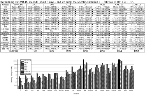
Table 3: Comparison of leaves cardinality (mean±std.) on benchmark datasets.•/◦indicates that our WODT generates fewer/more leaf nodes than the corresponding method (pairwiset-tests at95%significance level). ‘N/A’ means that no results were obtained after running out 250000 seconds (about 3 days), and we adopt the scientific notationa±b(Ec)=a×10c±b×10c.
dataset our WODT APDT CO2 CO2r OC1 OC1r CART-LC CART-LCr
iris .5200±.1170(E1) .7800±.1200(E1)• .8000±.0200(E1)• .1500±.0000(E2)• .5400±.0699(E1) .5589±.1440(E2)• .6500±.0900(E1) .1080±.0343(E3)•
wine .3400±.0490(E1) .7500±.1100(E1)• .7500±.5200(E1)• .2710±.1095(E2)• .5100±.1200(E1)• .3730±.3080(E2)• .5100±.1600(E1)• .8400±.6500(E1)•
glass .4620±.0240(E2) .3620±.0220(E2)◦ .3620±.0250(E2)◦ .2976±.0842(E3)• .8120±.4630(E2)• .3566±.0462(E3)• .5280±.2380(E2) .5901±.0662(E3)•
heart .2320±.0412(E2) .3429±.0279(E2)• .3429±.0520(E2)• .9797±.0862(E3)• .7120±.4700(E2)• .1949±.0467(E3)• .9090±.3660(E2)• .3639±.0598(E3)•
breast .1400±.0210(E2) .2320±.0200(E2)• .2390±.0960(E2)• .5391±.1154(E3)• .3279±.2910(E2)• .9020±.4100(E2)• .4610±.1889(E2)• .1943±.0458(E3)•
diabetes .1082±.0044(E3) .1041±.0047(E3)◦ .1049±.0226(E3) .1841±.0256(E4)• .1409±.0940(E3) .4521±.1076(E3)• .1565±.0367(E3)• .9519±.0910(E3)•
vehicle .1140±.0087(E3) .1055±.0031(E3)◦ .2236±.0105(E3)• .1508±.0172(E4)• .1840±.0895(E3) .6143±.1993(E3)• .2148±.0539(E3)• .1133±.0098(E4)•
fourclass .1860±.0242(E2) .2170±.0240(E2)• .2320±.0540(E2)• .3289±.1830(E2)• .2950±.1920(E2) .4360±.2680(E2)• .1989±.1250(E2) .4520±.2420(E2)•
segment .6419±.0248(E2) .5570±.0279(E2)◦ .2232±.1011(E3)• .3252±.1256(E3)• .1108±.0537(E3)• .3972±.1203(E3)• .8800±.2849(E2)• .7347±.1109(E3)•
dna .1601±.0170(E2) .1194±.0094(E3)• .4130±.1079(E3)• .5216±.1290(E3)• .1723±.0147(E3)• .2904±.0222(E3)• .1242±.0211(E3)• .3371±.0214(E3)•
satimage .2103±.0121(E3) .3298±.0278(E3)• .6102±.0736(E3)• .5791±.0354(E4)• .5258±.1346(E3)• .1913±.0144(E4)• .5137±.0719(E3)• .2818±.0198(E4)•
usps .1500±.0096(E3) .3389±.0517(E3)• N/A .5295±.0964(E4)• .5100±.0073(E3)• .9744±.0367(E3)• .6143±.0974(E3)• .1227±.0022(E4)•
pendigits .1494±.0407(E3) .2094±.0597(E3)• .1508±.0502(E3) .3315±.0760(E3)• .3970±.0050(E3)• .1107±.0150(E4)• .1941±.0424(E3)• .1890±.0121(E4)•
letter .1213±.0023(E4) .1752±.0063(E4)• .1198±.0167(E4) .1787±.0171(E4)• .2083±.0100(E4)• .1056±.0020(E5)• .1804±.0122(E4)• .1610±.0025(E5)•
protein .4572±.0173(E3) .2849±.0050(E4)• .3044±.0031(E4)• .4398±.0003(E5)• .3329±.1120(E4)• .1502±.0054(E4)• .3165±.0017(E4)• .1586±.0058(E4)•
shuttle .8115±.0363(E2) .2739±.0409(E2)◦ .1459±.0589(E3)• .3091±.0855(E3)• .3979±.2100(E2)◦ .4869±.1146(E3)• .3410±.0310(E2)◦ .8264±.0474(E3)•
connect4 .2976±.0069(E4) .9700±.0657(E4)• .1388±.0054(E5)• .5242±.0000(E5)• .1041±.0296(E5)• .6458±.2000(E4)• .1065±.0074(E5)• .7490±.0254(E4)•
mnist .7371±.0270(E3) .3329±.0167(E4)• N/A N/A .2500±.0119(E4)• .2032±.0002(E4)• .3279±.0118(E4)• .1910±.0020(E4)•
ijcnn1 .7180±.0078(E3) .8742±.2904(E3)• .1566±.0218(E4)• .2327±.0016(E5)• .1724±.1793(E3)◦ .1006±.0937(E4)• .1611±.0181(E4)• .9714±.0205(E4)•
cod-rna .7743±.0031(E4) .2751±.0174(E4)◦ .9501±.5928(E3)◦ .1000±.0000(E3)◦ .7283±.0290(E4)◦ .1240±.0280(E5)• .9594±.1264(E3)◦ .1535±.0121(E5)•
win/tie/loss 14/0/6 15/3/2 19/0/1 13/4/3 20/0/0 15/3/2 20/0/0
iris wine glass heart breast diabetes vehicle fourclass segment dna satimage usps pendigits letter protein shuttle connect4 mnist ijcnn1 cod-rna
0.01 0.1 1 10 100 1000 10000 100000
T
r
a
i
n
i
n
g
t
i
m
e
(
s
e
c
o
n
d
s
)
Datasets our WODT
APDT CO2 CO2r OC1 OC1r CART-LC CART-LCr
Figure 1: Comparison of the running time (in seconds) of WODT and other decision trees on benchmark datasets. Notice that the
y-axis is in log-scale. Full black columns imply that no results were returned after running out 250000 seconds (about 3 days).
OC1 and CART-LC, though these oblique decision trees are accompanied with the best axis-parallel splitting initialization in the implementation. In comparison with the axis-parallel decision tree (APDT) method, our proposed WODT method achieves comparable performance for small-size datasets, and shows its superior for datasets of size larger than5000, such assatimageandpendigits.
Table 3 shows the comparisons of leaves cardinality of our WODT with other methods. As can be seen, our WODT has fewer leaves than the oblique decision trees with random initialization such as CO2r, OC1r and CART-LCr, except for datasetcod-rna. We think that CO2r gets invalid partitons repeatedly until this method runs up to the maximal depth and returns with a deep and thin tree, which results in such few leaves. This analysis is also supported in Table 2 that our WODT method and CO2r achieve accuracy rates of 0.9543 and 0.6667, respectively.
It is also observable, from Table 3, that our WODT method has fewer, or as many leaves as those oblique decision trees with the best axis-parallel splitting initialization. Moreover, we notice that the previous oblique decision trees are not easy to obtain small-size trees without the best axis-parallel
splitting initialization, and the oblique decision trees with random initialization could produce more leaves, which may cause overfitting and take relatively poor performance as shown in Table 2.
We also compare the running time of WODT and the other decision tree methods, and the average CPU time (in sec-onds) is shown in Figure 1. As can be seen, our WODT takes comparable running time with the traditional axis-parallel decision tree (APDT) method. It is also observable that our WODT takes much less running time than the state-of-the-art oblique decision trees with the best axis-parallel splitting ini-tialization or random iniini-tialization in most cases. In particular, our WODT is about 100 times faster than the other decision tree methods for the datasets of feature dimensionality larger than200, such asusps,proteinandmnist.
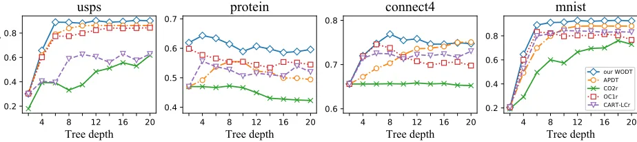
Depth Analysis
We finally analyze the influence of tree depths. Due to page limitation, we only present empirical results on four datasets
4 8 12 16 20
Tree depth
0.2 0.4 0.6 0.8
Te
st a
cc
ura
cy
usps
4 8 12 16 20
Tree depth
0.4 0.5 0.6
0.7
protein
4 8 12 16 20
Tree depth
0.6 0.7
0.8
connect4
4 8 12 16 20
Tree depth
0.2 0.4 0.6 0.8
mnist
our WODT APDT CO2r OC1r CART-LCr
Figure 2: The influence on test accuracy with respect to tree depths for different methods.
4 8 12 16 20
Tree depth
0.2 0.4 0.6 0.8 1.0
Tra
ini
ng a
cc
ura
cy
usps
4 8 12 16 20
Tree depth
0.5 0.6 0.7 0.8 0.9
1.0
protein
4 8 12 16 20
Tree depth
0.7 0.8 0.9
1.0
connect4
4 8 12 16 20
Tree depth
0.2 0.4 0.6 0.8
1.0
mnist
our WODT APDT CO2r OC1r CART-LCr
Figure 3: The influence on training accuracy with respect to tree depths for different methods.
Figure 2 shows the relationships between test accuracies and tree depths. Here the tree depth ranges from 2 to 20 with interval 2, and we compare our WODT with four decision trees: APDT, CO2r, OC1 and CART-LCr for simplicity, and the trends are similar to other methods such as CO2, OC1 and CART-LC. As can be seen, our WODT achieves the best performance at different depths in comparison with the other four methods, and it is also observable that our WODT method tends to achieve better generalization performance only with a shallow decision tree.
Figure 3 shows the relationships between the training ac-curacies and tree depths, where the range and compared methods are similar to those of Figure 2. As can be seen, our WODT method achieves better training accuracies than the others, which shows its stronger ability to fit data of our method. It is noteworthy that our WODT method and axis-parallel decision tree (APDT) method well fit datasetusps
andmnistat a depth of20while WODT achieves better test accuracies as shown in Figure 2. This illustrates that optimiz-ing the objective function in this work could yield a robust split by considering weighted entropy.
Conclusions
Oblique decision trees have attracted much attention during the past decades, and previous decision trees rely on the best axis-parallel splitting initialization with high computational cost. This work presents new Weighted Oblique Decision Tree (WODT). The basic idea is motivated from the weighted entropy, and we optimize the continuous and differentiable objective function with random initialization to find the split for each internal node. Extensive experiments show the
ef-fectiveness and robustness of our proposed method. In the future, an interesting work is to construct oblique decision trees based on ‘sparse’ splits by optimizing our objective function under the`1penalty, which may present better inter-pretability and efficiency for prediction. Another interesting future work is to construct ensemble methods, such as ran-dom forests and boosting, based on our WODT method.
References
Abuzaid, F.; Bradley, J. K.; Liang, F. T.; Feng, A.; Yang, L.; Zaharia, M.; and Talwalkar, A. S. 2016. Yggdrasil: An optimized system for training deep decision trees at scale. InAdvances in Neural Information Processing Systems 31, 3817–3825.
Amasyali, M. F., and Ersoy, O. 2008. Cline: A new decision-tree family. IEEE Transactions on Neural Networks 19(2):356–363.
Bennett, K. P., and Blue, J. A. 2002. A support vector machine approach to decision trees. InProceedings of the IEEE International Joint Conference on Neural Networks, 2396–2401.
Bosch, A.; Zisserman, A.; and Munoz, X. 2007. Image classification using random forests and ferns. InProceedings of the IEEE International Conference on Computer Vision, 1–8.
Breiman, L. I.; Friedman, J. H.; Olshen, R. A.; and Stone, C. J. 1984. Classification and Regression Trees (CART). Encyclopedia of Ecology40(3):582–588.
Brodley, and Utgoff, P. 1995. Multivariate decision trees. Machine Learning19(1):45–77.
Cicalese, F.; Laber, E.; and Saettler, A. M. 2014. Diagno-sis determination: Decision trees optimizing simultaneously worst and expected testing cost. InProceedings of the 31st International Conference on Machine Learning, 414–422.
Domingos, P., and Hulten, G. 2000. Mining high-speed data streams. InProceedings of the 6th ACM SIGKDD Conference on Knowledge Discovery and Data Mining, 71–80.
Fan, L. 2016. Accurate robust and efficient error estimation for decision trees. InProceedings of the 33rd International Conference on Machine Learning, 239–247.
Friedman, J. H. 2001. Greedy function approximation: A gradient boosting machine. Annals of Statistics29(5):1189– 1232.
Fuhr, N., and Pfeifer, U. 1994. Probabilistic information retrieval as a combination of abstraction, inductive learn-ing, and probabilistic assumptions. ACM Transactions on Information Systems12(1):92–115.
Geurts, P.; Ernst, D.; and Wehenkel, L. 2006. Extremely randomized trees. Machine Learning63(1):3–42.
Guias¸u, S. 1971. Weighted entropy.Reports on Mathematical Physics2(3):165–179.
Guo, H., and Gelfand, S. B. 1992. Classification trees with neural network feature extraction. IEEE Transactions on Neural Networks3(6):923–933.
Heath, D.; Kasif, S.; and Salzberg, S. 1993. Induction of oblique decision trees. InProceedings of the 13th Interna-tional Joint Conference on Artificial Intelligence, 1002–1007. Kontschieder, P.; Fiterau, M.; Criminisi, A.; and Rota Bulo, S. 2015. Deep neural decision forests. InProceedings of the IEEE International Conference on Computer Vision, 1467–1475.
Loh, W.-Y., and Shih, Y.-S. 1997. Split selection methods for classification trees.Statistica Sinica7(4):815–840.
L´opez-Chau, A.; Cervantes, J.; L´opez-Garc´ıa, L.; and Lam-ont, F. G. 2013. Fisher’s decision tree.Expert Systems with Applications40(16):6283–6291.
Manwani, N., and Sastry, P. S. 2012. Geometric decision tree. IEEE Transactions on Systems, Man, and Cybernetics 42(1):181–92.
Messenger, R., and Mandell, L. 1972. A modal search technique for predictive nominal scale multivariate analysis. Journal of the American Statistical Association67(340):768– 772.
Murthy, S. K.; Kasif, S.; and Salzberg, S. 1994. A system for induction of oblique decision trees. Journal of Artificial Intelligence Research2(1):1–32.
Norouzi, M.; Collins, M. D.; Fleet, D. J.; and Kohli, P. 2015. CO2 forest: Improved random forest by continuous opti-mization of oblique splits.arXiv preprint arXiv:1506.06155, 2015.
Quinlan, J. R. 1986. Induction of decision trees. Machine Learning1(1):81–106.
Quinlan, J. R. 1993. C4.5: Programs for Machine Learning. Morgan Kaufmann Publishers.
Robertson, B.; Price, C.; and Reale, M. 2013. CARTopt: A random search method for nonsmooth unconstrained op-timization. Computational Optimization and Applications 56(2):291–315.
Setiono, R., and Liu, H. 1999. A connectionist approach to generating oblique decision trees. IEEE Transactions on Systems, Man, and Cybernetics29(3):440–444.
Shotton, J.; Girshick, R.; Fitzgibbon, A.; Sharp, T.; Cook, M.; Moore, R.; Moore, R.; Kohli, P.; Criminisi, A.; and Kipman, A. 2013a. Efficient human pose estimation from single depth images.IEEE Transactions on Pattern Analysis and Machine Intelligence35(12):2821–2840.
Shotton, J.; Sharp, T.; Kohli, P.; Nowozin, S.; Winn, J.; and Criminisi, A. 2013b. Decision jungles: Compact and rich models for classification. InAdvances in Neural Information Processing Systems 28, 234–242.
Str¨omberg, J.-E.; Zrida, J.; and Isaksson, A. 1991. Neural trees-using neural nets in a tree classifier structure. In Pro-ceedings of the IEEE International Conference on Acoustics, Speech and Signal Processing, 137–140.
Zhou, Z.-H., and Chen, Z.-Q. 2002. Hybrid decision tree. Knowledge-Based Systems15(8):515–528.
Zhou, Z.-H., and Feng, J. 2017. Deep forest: Towards an alternative to deep neural networks. InProceedings of the 26th International Joint Conference on Artificial Intelligence, 3553–3559.