The Thirty-Third AAAI Conference on Artificial Intelligence (AAAI-19)
Tensor Ring Decomposition with Rank Minimization on
Latent Space: An Efficient Approach for Tensor Completion
Longhao Yuan,
1,2Chao Li,
2Danilo Mandic,
5Jianting Cao,
1,2,4,†Qibin Zhao
2,3,†1Graduate School of Engineering, Saitama Institute of Technology, Japan
2Tensor Learning Unit, RIKEN Center for Advanced Intelligence Project (AIP), Japan
3School of Automation, Guangdong University of Technology, China
4School of Computer Science and Technology, Hangzhou Dianzi University, China
5Department of Electrical and Electronic Engineering, Imperial College London, United Kingdom
Abstract
In tensor completion tasks, the traditional low-rank tensor de-composition models suffer from the laborious model selec-tion problem due to their high model sensitivity. In particu-lar, for tensor ring (TR) decomposition, the number of model possibilities grows exponentially with the tensor order, which makes it rather challenging to find the optimal TR decom-position. In this paper, by exploiting the low-rank structure of the TR latent space, we propose a novel tensor comple-tion method which is robust to model seleccomple-tion. In contrast to imposing the low-rank constraint on the data space, we in-troduce nuclear norm regularization on the latent TR factors, resulting in the optimization step using singular value de-composition (SVD) being performed at a much smaller scale. By leveraging the alternating direction method of multipli-ers (ADMM) scheme, the latent TR factors with optimal rank and the recovered tensor can be obtained simultaneously. Our proposed algorithm is shown to effectively alleviate the bur-den of TR-rank selection, thereby greatly reducing the com-putational cost. The extensive experimental results on both synthetic and real-world data demonstrate the superior per-formance and efficiency of the proposed approach against the state-of-the-art algorithms.
Introduction
Tensor decompositions aim to find latent factors in tensor-valued data (i.e., the generalization of multi-dimensional arrays), thereby casting large-scale and intractable tensor problems into a multilinear tensor latent space of low-dimensionality (very few degrees of freedom designated by the rank). The latent factors within tensor decomposition can be considered as the latent features of data, which makes them an ideal set of bases to predict missing entries when the acquired data is incomplete. The specific forms and op-erations among latent factors determine the type of sor decomposition. The most classical and successful ten-sor decomposition models are the Tucker decomposition
Copyright c2019, Association for the Advancement of Artificial Intelligence (www.aaai.org). All rights reserved.
This work was supported by JSPS KAKENHI (Grant No. 17K00326, 15H04002, 18K04178), JST CREST (Grant No. JP-MJCR1784), and the National Natural Science Foundation of China (Grant No. 61773129).
The code is available at: https://github.com/yuanlonghao/TRLRF †
Corresponding authors: [email protected], [email protected]
(TKD) and the CANDECOMP/PARAFAC (CP) decompo-sition (Kolda and Bader 2009). More recently, the matrix product state/tensor-train (MPS/TT) decomposition has be-come very attractive, owing to its super-compression and computational efficiency properties (Oseledets 2011). Cur-rently, a generalization of TT decomposition, termed the tensor ring (TR) decomposition, has been studied across scientific disciplines (Zhao et al. 2016a; 2018). These ten-sor decomposition models have found application in var-ious fields such as machine learning (Wang et al. 2018; Novikov et al. 2015; Anandkumar et al. 2014; Kanagawa et al. 2016), signal processing (Cong et al. 2015), image/video completion (Liu et al. 2013; Zhao et al. 2016b), compressed sensing (Gandy, Recht, and Yamada 2011), to name but a few. Tensor completion is one of the most important appli-cations of tensor decompositions, with the goal to recover an incomplete tensor from partially observed entries. The theo-retical lynchpin in tensor completion problems is the tensor low-rank assumption, and the methods can mainly be cate-gorized into two types: (i) tensor-decomposition-based ap-proach and (ii) rank-minimization-based apap-proach.
Tensor decomposition based methods find latent factors of tensor by the incomplete tensor, and then the latent fac-tors are used to predict the missing entries. Many comple-tion algorithms have been proposed based on alternating least squares (ALS) method (Grasedyck, Kluge, and Kramer 2015; Wang, Aggarwal, and Aeron 2017), gradient-based method (Yuan, Zhao, and Cao 2017; Acar et al. 2011), to mention but a few. Though ALS and gradient-based algo-rithms are free from burdensome hyper-parameter tuning, the performance of these algorithms is rather sensitive to model selection, i.e., rank selection of the tensor decompo-sition. Moreover, since the optimal rank is generally data-dependent, it is very challenging to specify the optimal rank beforehand. This is especially the case for Tucker, TT, and TR decompositions, for which the rank is defined as a vec-tor; it is therefore impossible to find the optimal ranks by cross-validation due to the immense possibilities.
differ-ent definitions of tensor rank, various nuclear norm reg-ularized algorithms have been proposed (Liu et al. 2013; Imaizumi, Maehara, and Hayashi 2017; Liu et al. 2014; 2015). Rank minimization based methods do not need to specify the rank of the employed tensor decompositions be-forehand, and the rank of the recovered tensor will be au-tomatically learned from the limited observations. However, these algorithms face multiple large-scale singular value de-composition (SVD) operations on the 2D unfoldings of the tensor when employing the nuclear norm and numerous hyper-parameter tuning, which in turn leads to high com-putational cost and low efficiency.
To address the problems of high sensitivity to rank se-lection and low computational efficiency which are inherent in traditional tensor completion methods, in this paper, we propose a new algorithm named tensor ring low-rank fac-tors (TRLRF) which effectively alleviates the burden of rank selection and reduces the computational cost. By virtue of employing both nuclear norm regularization and tensor de-composition, our model provides performance stability and high computational efficiency. The proposed TRLRF is ef-ficiently solved by the ADMM algorithm and it simulta-neously achieves both the underlying tensor decomposition and completion based on TR decomposition. Our main con-tributions in this paper are:
• A theoretical relationship between the multilinear tensor rank and the rank of TR factors is established, which al-lows the low-rank constraint to be performed implicitly on TR latent space. This has led to fast SVD calculation on small size factors.
• The nuclear norm is further imposed to regularize the TR-ranks, which enables our algorithm to always obtain a sta-ble solution, even if the TR-rank is inappropriately given. This highlights rank-robustness of the proposed TRLRF algorithm.
• An efficient algorithm based on ADMM is developed to optimize the proposed model, so as to obtain the TR-factors and the recovered tensor simultaneously.
Preliminaries and Related Works
Notations
The notations in (Kolda and Bader 2009) are adopted in this paper. A scalar is denoted by a standard lowercase letter or an uppercase letter, e.g.,x, X ∈ R, and a vector is de-noted by a boldface lowercase letter, e.g.,x ∈ RI. A
ma-trix is denoted by a boldface capital letter, e.g.,X∈RI×J.
A tensor of order N ≥ 3 is denoted by calligraphic let-ters, e.g., X ∈ RI1×I2×···×IN. The set {X(n)}N
n=1 :=
{X(1),X(2), . . . ,X(N)} denotes a tensor sequence, with X(n) being then-th tensor of the sequence. Where
appro-priate, a tensor sequence can also be written as [X]. The representations of matrix sequences and vector sequences are designated in the same way. An element of a tensor X ∈ RI1×I2×···×IN of index (i
1, i2, . . . , iN) is denoted
byX(i1, i2, . . . , iN)orxi1i2...iN. The inner product of two tensorsX,Y with the same sizeRI1×I2×···×IN is defined
ashX,Yi=P
i1
P
i2· · ·
P
iNxi1i2...iNyi1i2...iN. Further-more, the Frobenius norm of X is defined by kXkF = p
hX,Xi.
We employ two types of tensor unfolding (matricization) operations in this paper. The standard mode-n unfolding (Kolda and Bader 2009) of tensor X ∈ RI1×I2×···×IN is denoted by X(n) ∈ RIn×I1···In−1In+1···IN. Another mode-n unfolding of tensorX which is often used in TR operations (Zhao et al. 2016a) is denoted by X<n> ∈
RIn×In+1···INI1···In−1. Furthermore, the inverse operation of unfolding is matrix folding (tensorization), which trans-forms matrices to higher-order tensors. In this paper, we only define the folding operation for the first type of mode-n unfolding as foldn(·), i.e., for a tensor X, we have
foldn(X(n)) =X.
Tensor ring decomposition
The tensor ring (TR) decomposition is a more general de-composition model than the tensor-train (TT) decomposi-tion. It represents a tensor of higher-order by circular multi-linear products over a sequence of low-order latent core ten-sors, i.e., TR factors. Forn= 1, . . . , N, the TR factors are denoted byG(n)∈
RRn×In×Rn+1and each consists of two rank-modes (i.e., mode-1and mode-3) and one dimension-mode (i.e., dimension-mode-2). The syntax {R1, R2, . . . , RN+1}
de-notes the TR-rank which controls the model complexity of TR decomposition. The TR decomposition applies trace op-erations and all of the TR factors are set to be 3rd-order; thus the TR decomposition relaxes the rank constraint on the first and last core of TT toR1 =RN+1. Moreover, TR
decom-position linearly scales to the order of the tensor, and in this way it overcomes the ‘curse of dimensionality’. In this case, TR can be considered as a linear combination of TTs and hence offers a powerful and generalized representation abil-ity. The element-wise relation of TR decomposition and the generated tensor is given by:
X(i1, i2, . . . , iN) =Trace
( N Y
n=1
G(in) n
)
, (1)
where Trace{·} is the matrix trace operation, G(in)
n ∈
RRn×Rn+1 is theinth mode-2slice matrix ofG(n), which
can also be denoted byG(n)(:, in,:)according to the Matlab
notation.
Tensor completion
Completion by TR decomposition Tensor
2015), TRWOPT (Yuan et al. 2018) and TRALS (Wang, Ag-garwal, and Aeron 2017). To the best of our knowledge, there are two proposed TR-based tensor completion algo-rithms: the TRALS and TRWOPT. They apply the same op-timization model which is formulated as:
min
[G]
kPΩ(T −Ψ([G]))k2F, (2)
where the optimization objective is the TR factors, [G], PΩ(T)denotes all the observed entries w.r.t. the set of
in-dices of observed entries represented byΩ, andΨ([G]) de-notes the approximated tensor generated by[G]. Every ele-ment ofΨ([G])is calculated by equation (1). The two algo-rithms are both based on the model in (2). However, TRALS applies alternative least squares (ALS) method and TR-WOPT uses a gradient-based algorithm to solve the model, respectively. They perform well for both low-order and high-order tensors due to the high representation ability and flex-ibility of TR decomposition. However, these algorithms are shown to suffer from high sensitiveness to rank selection, which would lead to high computational cost.
Completion by nuclear norm regularization The model
of rank minimization-based tensor completion can be for-mulated as:
min
X Rank(X) +
λ
2kPΩ(T −X)k
2
F, (3)
whereX is the recovered low-rank tensor, and Rank(·)is a rank regularizer. The model can therefore find the low-rank structure of the data and approximate the recovered tensor. Because determining the tensor rank is an NP-hard problem (Hillar and Lim 2013; Kolda and Bader 2009), work in (Liu et al. 2013) and (Signoretto et al. 2014) extends the concept of low-rank matrix completion and defines tensor rank as a sum of the rank of mode-nunfolding of the object ten-sor. Moreover, the convex surrogate named nuclear norm is applied to the tensor low-rank model and it simultaneously regularizes all the mode-nunfoldings of the object tensor. In this way, the model in (3) can be reformulated as:
min
X
N
X
n=1
kX(n)k∗+ λ
2kPΩ(T −X)k
2
F, (4)
wherek · k∗denotes the nuclear norm regularization in the
form of a sum of the singular values of the matrix. Usually, the model is solved by ADMM algorithms and it is shown to have fast convergence and good performance when data size is small. However, when dealing with large-scale data, the multiple SVD operations in the optimization step will be intractable due to high computational cost.
Tensor Ring Low-rank Factors
To solve the issues traditional tensor completion methods have, we impose low-rankness on each of the TR factors and so that our basic tensor completion model is formulated as follow:
min
[G],X
N
X
n=1
kG(n)k∗+ λ
2kX −Ψ([G])k
2
F,
s.t. PΩ(X) =PΩ(T).
(5)
To solve (5), we first need to deduce the relation of the tensor rank and the corresponding core tensor rank, which can be explained by the following theorem.
Theorem 1. Given an N-th order tensor X ∈
RI1×I2×···×IN which can be represented by equation (1),
then the following inequality holds for alln= 1, . . . , N:
Rank(G((2)n))≥Rank(X(n)). (6)
Proof. For then-th core tensorG(n), according to the work
in (Zhao et al. 2016a), we have:
X<n>=G
(n) (2)(G
(6=n)
<2>)>, (7)
whereG(6=n)∈RRn+1×
QN
i=1,i6=nIi×Rnis a subchain tensor generated by merging all but then-th core tensor. Hence, the relation of the rank satisfies:
Rank(X<n>)≤min{Rank(G
(n)
(2)),Rank(G (6=n)
<n>)}
≤Rank(G((2)n)).
(8)
The proof is completed by
Rank(X<n>) =Rank(X(n))≤Rank(G (n)
(2)). (9)
This theorem proves the relation between the tensor rank and the rank of the TR factors. The rank of mode-n unfold-ing of the tensor X is upper bounded by the rank of the dimension-mode unfolding of the corresponding core tensor G(n), which allows us to impose a low-rank constraint on
G(n)
. By the new surrogate, our model (5) is reformulated by:
min
[G],X
N
X
n=1
kG((2)n)k∗+ λ
2kX −Ψ([G])k
2
F
s.t. PΩ(X) =PΩ(T).
(10)
The above model imposes nuclear norm regularization on the dimension-mode unfoldings of the TR factors, which can largely decrease the computational complexity compared to the algorithms which are based on model (4). Moreover, we consider to give low-rank constraints on the two rank-modes of the TR factors, i.e., the unfoldings of the TR fac-tors along mode-1and mode-3, which can be expressed by
PN
n=1kG (n) (1)k∗+
PN
n=1kG (n)
(3)k∗. When the model is
opti-mized, nuclear norms of the rank-mode unfoldings and the fitting error of the approximated tensor are minimized simul-taneously, resulting in the initial TR-rank becoming the up-per bound of the real TR-rank of the tensor, thus equipping our model with robustness to rank selection. The tensor ring low-rank factors (TRLRF) model can be finally expressed as:
min
[G],X
N
X
n=1 3
X
i=1
kG((ni))k∗+ λ
2kX−Ψ([G])k
2
F
s.t. PΩ(X) =PΩ(T).
Our TRLRF model has two distinctive advantages. Firstly, the low-rank assumption is placed on tensor factors instead of on the original tensor, this greatly reduces the compu-tational complexity of the SVD operation. Secondly, low-rankness of tensor factors can enhance the robustness to rank selection, which can alleviate the burden of searching for optimal TR-rank and reduce the computational cost in the implementation.
Solving scheme
To solve the model in (11), we apply the alternating di-rection method of multipliers (ADMM) which is efficient and widely used (Boyd et al. 2011). Moreover, because the variables of TRLRF model are inter-dependent, we impose auxiliary variables to simplify the optimization. Thus, the TRLRF model can be rewritten as
min
[M],[G],X
N
X
n=1 3
X
i=1
kM((n,ii) )k∗+ λ
2kX −Ψ([G])k
2
F,
s.t.M((n,ii) )=G((ni)), n= 1, . . . , N, i= 1,2,3, PΩ(X) =PΩ(T),
(12)
where[M] :={M(n,i)}N,n=13,i=1are the auxiliary variables of [G]. By merging the equal constraints of the auxiliary variables into the Lagrangian equation, the augmented La-grangian function of TRLRF model becomes
L([G],X,[M],[Y])
=
N
X
n=1 3
X
i=1
kM((n,ii) )k∗+<Y(n,i),M(n,i)−G(n)>
+µ
2kM
(n,i)−G(n)k2
F
+λ
2kX−Ψ([G])k
2
F,
s.t. PΩ(X) =PΩ(T),
(13) where[Y] :={Y(n,i)}N,3
n=1,i=1are the Lagrangian
multipli-ers, andµ > 0is a penalty parameter. Forn = 1, . . . , N, i = 1,2,3,G(n),M(n,i)andY(n,i)are each independent, so we can update them by the updating scheme below.
Update ofG(n). By using (13), the augmented Lagrangian
function w.r.t.G(n)can be simplified as
L(G(n)) =
3
X
i=1
µ 2
M
(n,i)
−G(n)+ 1 µY
(n,i)
2
F
+λ
2
X −Ψ([G])
2
F+CG,
(14)
where the constant CG consists of other parts of the
La-grangian function which is irrelevant to updatingG(n). This
is a least squares problem, so forn= 1, . . . , N,G(n)can be updated by
G(+n)=fold2
X3
i=1
(µM((2)n,i)+Y((2)n,i))
+λX<n>G
(6=n)
<2>
λG<(6=2n>),TG<(6=2n>)+ 3µI−1, (15)
whereI∈RR
2
n×Rn2 denotes the identity matrix.
Update of M(n,i). Fori = 1,2,3, the augmented
La-grangian functions w.r.t.[M]is expressed as
L(M(n,i)) =µ 2
M
(n,i)
−G(n)+ 1 µY
(n,i)
2
F
+M
(n,i) (i)
∗+CM.
(16)
The above formulation has a closed-form (Cai, Cand`es, and Shen 2010), which is given by
M(+n,i)=foldi
D1
µ G
(n) (i) −
1 µY
(n,i) (i)
, (17)
whereDβ(·)is the singular value thresholding (SVT)
oper-ation, e.g., ifUSVT is the singular value decomposition of
matrixA, thenDβ(A) =Umax{S−βI,0}VT.
Update ofX. The augmented Lagrangian functions w.r.t.
X is given by
L(X) = λ 2
X −Ψ([G])
2
F+CX,
s.t. PΩ(X) =PΩ(T),
(18)
which is equivalent to the tensor decomposition based model in (2). The expression forX is updated by inputing the ob-served values in the corresponding entries, and by approx-imating the missing entries by updated TR factors [G] for every iteration, i.e.,
X+=PΩ(T) +PΩ¯(Ψ([G])), (19)
whereΩ¯ is the set of indices of missing entries which is a complement toΩ.
Update ofY(n,i). Forn = 1, . . . , N andi = 1,2,3, the
Lagrangian multiplierY(n,i)is updated as
Y(+n,i)=Y(n,i)+µ M(n,i)−G(n)
. (20)
In addition, the penalty term of the Lagrangian functionsL is restricted byµwhich is also updated for every iteration byµ+ =max{ρµ, µmax}, where1 < ρ <1.5is a tuning
hyper parameter.
The ADMM based solving scheme is updated iteratively based on the above equations. Moreover, we consider to set two optimization stopping conditions: (i) maximum number of iterationskmaxand (ii) the difference between two
itera-tions (i.e.,kX −XlastkF/kXkF) which is thresholded by
the tolerance tol. The implementation process and hyper-parameter selection of TRLRF is summarized in Algorithm 1. It should be noted that our TRLRF model is non-convex, so the convergence to the global minimum cannot be theo-retically guaranteed. However, the convergence of our algo-rithm can be verified empirically (see experiment details in Figure 1). Moreover, the extensive experimental results in the next section also illustrate the stability and effectiveness of TRLRF.
Computational complexity
0 20 40 60 80 100
Number of iteration (a)
0 5 10 15
Objective function
105
rank=2 rank=4 rank=8 rank=16
0 20 40 60 80 100
Number of iteration (b)
0 1 2 3 4
Objective function
107
=0.5 =5 =50 =500
Figure 1: Illustration of convergence for TRLRF under dif-ferent hyper-parameter choices. A synthetic tensor with TR structure (size7×8×7×8with TR-rank{4,4,4,4}, miss-ing rate 0.5) is tested. The experiment records the change of the objective function values along the number of itera-tions. Each independent experiment is conducted 100 times and the average results are shown in the graphs. Panels (a) and (b) represent the convergence curve when TR-rank and λare changed respectively.
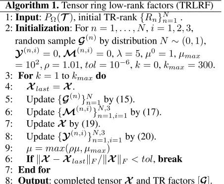
Algorithm 1.Tensor ring low-rank factors (TRLRF)
1:Input:PΩ(T), initial TR-rank{Rn}Nn=1.
2:Initialization: Forn= 1, . . . , N,i= 1,2,3, random sampleG(n)by distributionN∼(0,1),
Y(n,i)= 0,M(n,i)= 0,λ= 5,µ0= 1,µ
max
= 102, ρ= 1.01,tol= 10−6,k= 0,kmax= 300.
3: Fork= 1tokmaxdo
4: Xlast =X.
5: Update{G(n)}N
n=1by (15).
6: Update{M(n,i)}N,3
n=1,i=1by (17).
7: UpdateX by (19). 8: Update{Y(n,i)}N,3
n=1,i=1by (20).
9: µ=max(ρµ, µmax)
6: IfkX −XlastkF/kXkF < tol,break
7: End for
8: Output: completed tensorX and TR factors[G].
TR-rank is set asR1=R2=· · ·=RN =R, then the
com-putational complexity of updating [M] represents mainly the cost of SVD operation, which is O(PN
n=12InR3 +
I2
nR2). The computational complexities incurred
calculat-ingG(<6=2n>)and updating[G]areO(N R3QN
i=1,i6=nIi)and
O(N R2QN
i=1Ii+N R6), respectively. If we assumeI1=
I2 = · · · = IN = I, then overall complexity of our
pro-posed algorithm can be written asO(N R2IN +N R6). Compared to HaLRTC and TRALS which are the repre-sentative of the nuclear-norm-based and the tensor decom-position based algorithms, the computational complexity of HaLRTC is O(N IN+1). Since TRALS is based on ALS
method and TR decomposition, its computational complex-ity isO(P N R4IN +N R6), wherePdenotes the
observa-tion rate. We can see that the computaobserva-tional complexity of our TRLRF is similar to that of the two related algorithms. However, the desirable characteristic of rank selection
ro-bustness of our algorithm can help relieve the workload for model selection in practice, and thus the computational cost can be reduced. Moreover, though the computational com-plexity of TRLRF is of high power in R, due to the high representation ability and flexibility of TR decomposition, the TR-rank is always set as a small value. In addition, from experiments, we find out that our algorithm is capable of working efficiently for high-order tensors so that we can ten-sorize the data to a higher-order tensor and choose a small TR-rank to reduce the computational complexity.
Experimental Results
Synthetic data
We first conducted experiments to testify the rank robust-ness of our algorithm by comparing TRALS, TRWOPT, and our TRLRF. To verify the performance of the three algo-rithms, we tested two tensors of size 20×20×20×20
and7×8×7×8×7×8. The tensors were generated by TR factors of TR-ranks{6,6,6,6}and{4,4,4,4,4,4} re-spectively. The values of the TR factors were drawn from i.i.d. Gaussian distribution N ∼ (0,0.5). The observed entries of the tensors were randomly removed by a miss-ing rate of 0.5, where the missing rate is calculated by
1−M/num(Treal)andM is the number of sampled
en-tries (i.e., observed enen-tries). We recorded the completion performance of the three algorithms by selecting different TR-ranks. The evaluation index was RSE which is defined by RSE = kTreal−XkF/kTrealkF, whereTrealis the
known tensor with full observations andX is the recovered tensor calculated by each tensor completion algorithm. The hyper-parameters of our TRLRF were set according to Algo-rithm 1. All the hyper-parameters of TRALS and TRWOPT are set according to the recommended settings in the corre-sponding papers to get the best results.
2 4 6 8 10
TR-rank
10-6 10-4 10-2
100
RSE
(a)4th-order tensor
TRLRF TRALS TRWOPT
2 4 6 8 10
TR-rank
10-8
10-6 10-4
10-2 100
RSE
(b)6th-order tensor
TRLRF TRALS TRWOPT
Figure 2: Completion performance of three TR-based algo-rithms in the synthetic data experiment. The RSE values of different selected TR-ranks are recorded. The missing rate of the two target tensors equals0.5and the real TR-ranks are 6 and 4 respectively.
the performance of TRLRF remained stable while the per-formance of the other two compared algorithms fell dras-tically. This indicates that imposing low-rankness assump-tion on the TR factors can bring robustness to rank selecassump-tion, which largely alleviates the model selection problem in the experiments.
Benchmark images inpainting
Figure 3: The eight benchmark images. The first image is named “Lena” and is used in the next two experiments.
RSE =
0.19734 0.1398 0.11106 0.10673 0.10141 0.10109 0.20025 0.1286 0.23614 0.3596 0.50176 15.226
0.19725 0.12906 0.1358 0.16612 0.17618 0.26522
TR-rank(10)
TRLRF (proposal)
TRALS
TRWOPT
TR-rank(4) TR-rank(6) TR-rank(8) TR-rank(10) TR-rank(12)
RSE=0.1311 RSE=0.1111 RSE=0.1067 RSE=0.1014 RSE=0.1011
RSE=0.1286 RSE=0.2361 RSE=0.3596 RSE=0.5018 RSE=0.9522
RSE=0.1291 RSE=0.1358 RSE=0.1661 RSE=0.1762 RSE=0.2652
Figure 4: Visual completion results of the TRLRF (pro-posed), TRALS, and TRWOPT on image “Lena” with dif-ferent TR-ranks, when the missing rate is0.8. The selected TR-ranks are 4, 6, 8, 10, 12 respectively, from the first col-umn to the last colcol-umn. The RSE results are noted under each picture.
In this section, we tested our TRLRF against the state-of-the-art algorithms on eight benchmark images which are shown in Figure 3. The size of each RGB image was
256×256×3which can be considered as a 3rd-order tensor. For the first experiment, we continued to verify the TR-rank robustness of TRLRF on the image named “Lena”. Figure 4 shows the completion results of TRLRF, TRALS, and TR-WOPT when different TR-ranks for each algorithm are se-lected. The missing rate of the image was set as0.8, which is the case that the TR decompositions are prone to overfitting. From the figure, we can see that our TRLRF gives better results than the other two TR-based algorithms in each case and the highest performance was obtained when the TR rank was set as 12. When TR-rank increases, the completion per-formance of TRALS and TRLRF decreases due to redundant
0.3 0.4 0.5 0.6 0.7 0.8 0.9
Missing rate 0
0.1 0.2 0.3 0.4 0.5 0.6 0.7 0.8 0.9 1
RSE
TRLRF TRALS TRWOPT TenALS FBCP HaLRTC TMac t-SVD
0.3 0.4 0.5 0.6 0.7 0.8 0.9
Missing rate 0
5 10 15 20 25 30 35
PSNR
TRLRF TRALS TRWOPT TenALS FBCP HaLRTC TMac t-SVD
Figure 5: Average completion performance of the eight con-sidered algorithms, under different data missing rates.
model complexity and overfitting of the algorithms, while our TRLRF shows better results even the selected TR-rank is larger than the desired TR-rank.
In the next experiment, we compared our TRLRF to the two TR-based algorithm, TRALS and TRWOPT, and the other state-of-the-art algorithms, i.e., TenALS (Jain and Oh 2014), FBCP (Zhao, Zhang, and Cichocki 2015), HaL-RTC (Liu et al. 2013), TMac (Xu et al. 2013) and t-SVD (Zhang et al. 2014). We tested these algorithms on all the eight benchmark images and for different missing rates: 0.3,0.4,0.5,0.6,0.7,0.8,0.9 and 0.95. The relative square error (RSE) and peak signal-to-noise ratio (PSNR) were adopted for the evaluation of the completion perfor-mance. For RGB image data, PSNR is defined as PSNR=
10 log10(2552/MSE)where MSE is calculated by MSE =
kTreal−Xk2F/num(Treal), and num(·) denotes the
num-ber of element of the fully observed tensor.
For the three based algorithms, we assumed the TR-ranks were equal for every core tensor (i.e., R1 = R2 =
. . . =RN). The best completion results for each algorithm
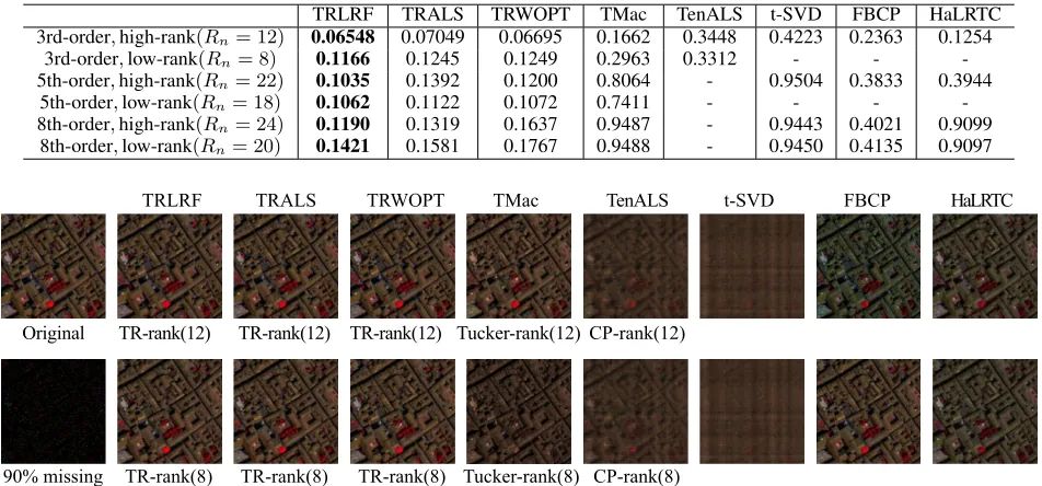
Table 1: HSI completion results (RSE) under three different tensor orders with different rank selections
TRLRF TRALS TRWOPT TMac TenALS t-SVD FBCP HaLRTC 3rd-order,high-rank(Rn= 12) 0.06548 0.07049 0.06695 0.1662 0.3448 0.4223 0.2363 0.1254
3rd-order,low-rank(Rn= 8) 0.1166 0.1245 0.1249 0.2963 0.3312 - -
-5th-order,high-rank(Rn= 22) 0.1035 0.1392 0.1200 0.8064 - 0.9504 0.3833 0.3944
5th-order,low-rank(Rn= 18) 0.1062 0.1122 0.1072 0.7411 - - -
-8th-order,high-rank(Rn= 24) 0.1190 0.1319 0.1637 0.9487 - 0.9443 0.4021 0.9099
8th-order,low-rank(Rn= 20) 0.1421 0.1581 0.1767 0.9488 - 0.9450 0.4135 0.9097
TRLRF TRALS TRWOPT TMac TenALS t-SVD FBCP HaLRTC
Original TR-rank(12) TR-rank(12) TR-rank(12) Tucker-rank(12) CP-rank(12)
90% missing TR-rank(8) TR-rank(8) TR-rank(8) Tucker-rank(8) CP-rank(8)
Figure 6: Completion results under the0.9missing rate HSI data. The channels 80, 34, 9 are picked to show the visual results. The rank selection of TRLRF, TRALS, TRWOPT, TMac and TenALS are given under the corresponding images.
Hyperspectral image
A hyperspectral image (HSI) of size200× 200×80which records an area of the urban landscape was tested in this sec-tion1. In order to test the performance of TRLRF on higher-order tensors, the HSI data was reshaped to higher-higher-order ten-sors, which is an easy way to find more low-rank features of the data. We compared our TRLRF to the other seven tensor completion algorithms in 3rd-order tensor (200×200×80), 5th-order tensor (10×20×10×20×80) and 8th-order ten-sor (8×5×5×8×5×5×8×10) cases. The higher-order tensors were generated from original HSI data by directly reshaping it to the specified size and order.
The experiment aims to verify the completion perfor-mance of the eight algorithms under different model selec-tion, whereby the experiment variables are the tensor order and tensor rank. The missing rates of all the cases are set as 0.9. All the tuning parameters of every algorithm were set according to the statement in the previous experiments. Besides, for the experiments which need to set rank manu-ally, we chose two different tensor ranks: high-rank and low-rank for algorithms. It should be noted that the CP-low-rank of TenALS and the Tucker-rank of TMac were set to the same values as TR-rank. The completion performance of RSE and visual results are listed in Table 1 and shown in Figure 6. The results of FBCP, HaLRTC and t-SVD were not affected by tensor rank, so the cases of the same order with differ-ent rank are left blank in Table 1. The TenALS could not deal with tensor more than three order, so the high-order
1
http://www.ehu.eus/ccwintco/index.php/Hyperspectral Remote Sensing Scenes
tensor cases for TenALS are also left blank. As shown in Ta-ble 1, our TRLRF gives the best recovery performance for the HSI image. In the 3rd-order cases, the best performance was obtained when the TR-rank was 12, however, when the rank was set to 8, the performance of TRLRF, TRALS, TR-WOPT, TMac, and TenALS failed because of the underfit-ting of the selected models. For 5th-order cases, when the rank increased from 18 to 22, the performance of TRLRF kept steady while the performance of TRALS, TRWOPT, and TMac decreased. This is because the high-rank makes the models overfit while our TRLRF performs without any issues, owing to its inherent TR-rank robustness. In the 8th-order tensor cases, similar properties can be obtained and our TRLRF also performed the best.
Conclusion
References
Acar, E.; Dunlavy, D. M.; Kolda, T. G.; and Mørup, M. 2011. Scalable tensor factorizations for incomplete data. Chemo-metrics and Intelligent Laboratory Systems106(1):41–56. Anandkumar, A.; Ge, R.; Hsu, D.; Kakade, S. M.; and Tel-garsky, M. 2014. Tensor decompositions for learning latent variable models.The Journal of Machine Learning Research
15(1):2773–2832.
Boyd, S.; Parikh, N.; Chu, E.; Peleato, B.; Eckstein, J.; et al. 2011. Distributed optimization and statistical learning via the alternating direction method of multipliers.Foundations and TrendsR in Machine learning3(1):1–122.
Cai, J.-F.; Cand`es, E. J.; and Shen, Z. 2010. A singular value thresholding algorithm for matrix completion. SIAM Journal on Optimization20(4):1956–1982.
Cong, F.; Lin, Q.-H.; Kuang, L.-D.; Gong, X.-F.; Astikainen, P.; and Ristaniemi, T. 2015. Tensor decomposition of EEG signals: a brief review. Journal of Neuroscience Methods
248:59–69.
Filipovi´c, M., and Juki´c, A. 2015. Tucker factorization with missing data with application to low-n-rank tensor com-pletion. Multidimensional Systems and Signal Processing
26(3):677–692.
Gandy, S.; Recht, B.; and Yamada, I. 2011. Tensor comple-tion and low-n-rank tensor recovery via convex optimiza-tion.Inverse Problems27(2):025010.
Grasedyck, L.; Kluge, M.; and Kramer, S. 2015. Vari-ants of alternating least squares tensor completion in the tensor train format. SIAM Journal on Scientific Computing
37(5):A2424–A2450.
Hillar, C. J., and Lim, L.-H. 2013. Most tensor problems are np-hard. Journal of the ACM (JACM)60(6):45.
Imaizumi, M.; Maehara, T.; and Hayashi, K. 2017. On ten-sor train rank minimization: Statistical efficiency and scal-able algorithm. InAdvances in Neural Information Process-ing Systems, 3933–3942.
Jain, P., and Oh, S. 2014. Provable tensor factorization with missing data. InAdvances in Neural Information Processing Systems, 1431–1439.
Kanagawa, H.; Suzuki, T.; Kobayashi, H.; Shimizu, N.; and Tagami, Y. 2016. Gaussian process nonparametric tensor estimator and its minimax optimality. InInternational Con-ference on Machine Learning, 1632–1641.
Kolda, T. G., and Bader, B. W. 2009. Tensor decompositions and applications. SIAM Review51(3):455–500.
Liu, J.; Musialski, P.; Wonka, P.; and Ye, J. 2013. Ten-sor completion for estimating missing values in visual data.
IEEE Transactions on Pattern Analysis and Machine Intelli-gence35(1):208–220.
Liu, Y.; Shang, F.; Fan, W.; Cheng, J.; and Cheng, H. 2014. Generalized higher-order orthogonal iteration for tensor de-composition and completion. InAdvances in Neural Infor-mation Processing Systems, 1763–1771.
Liu, Y.; Shang, F.; Jiao, L.; Cheng, J.; and Cheng, H. 2015. Trace norm regularized CANDECOMP/PARAFAC
decom-position with missing data.IEEE Transactions on Cybernet-ics45(11):2437–2448.
Novikov, A.; Podoprikhin, D.; Osokin, A.; and Vetrov, D. P. 2015. Tensorizing neural networks. InAdvances in Neural Information Processing Systems, 442–450.
Oseledets, I. V. 2011. Tensor-train decomposition. SIAM Journal on Scientific Computing33(5):2295–2317.
Signoretto, M.; Dinh, Q. T.; De Lathauwer, L.; and Suykens, J. A. 2014. Learning with tensors: a framework based on convex optimization and spectral regularization. Machine Learning94(3):303–351.
Wang, W.; Aggarwal, V.; and Aeron, S. 2017. Efficient low rank tensor ring completion. InIEEE International Confer-ence on Computer Vision (ICCV), 5698–5706. IEEE. Wang, W.; Sun, Y.; Eriksson, B.; Wang, W.; and Aggarwal, V. 2018. Wide compression: Tensor ring nets. In IEEE Conference on Computer Vision and Pattern Recognition (CVPR), 9329–9338. IEEE.
Xu, Y.; Hao, R.; Yin, W.; and Su, Z. 2013. Parallel matrix factorization for low-rank tensor completion.arXiv preprint arXiv:1312.1254.
Yuan, L.; Cao, J.; Wu, Q.; and Zhao, Q. 2018. Higher-dimension tensor completion via low-rank tensor ring de-composition.arXiv preprint arXiv:1807.01589.
Yuan, L.; Zhao, Q.; and Cao, J. 2017. Completion of high or-der tensor data with missing entries via tensor-train decom-position. InInternational Conference on Neural Information Processing, 222–229. Springer.
Zhang, Z.; Ely, G.; Aeron, S.; Hao, N.; and Kilmer, M. 2014. Novel methods for multilinear data completion and de-noising based on tensor-SVD. In Proceedings of the IEEE Conference on Computer Vision and Pattern Recog-nition, 3842–3849.
Zhao, Q.; Zhou, G.; Xie, S.; Zhang, L.; and Cichocki, A. 2016a. Tensor ring decomposition. arXiv preprint arXiv:1606.05535.
Zhao, Q.; Zhou, G.; Zhang, L.; Cichocki, A.; and Amari, S.-I. 2016b. Bayesian robust tensor factorization for incom-plete multiway data.IEEE Transactions on Neural Networks and Learning Systems27(4):736–748.
Zhao, Q.; Sugiyama, M.; Yuan, L.; and Cichocki, A. 2018. Learning efficient tensor representations with ring structure networks. In Sixth International Conference on Learning Representations (ICLR workshop).