Particle Gibbs Split-Merge Sampling for Bayesian Inference in Mixture Models

Particle Gibbs Split-Merge Sampling for Bayesian Inference

in Mixture Models

Alexandre Bouchard-Cˆot´e [email protected]

Department of Statistics University of British Columbia

Corresponding address: 3182 Earth Sciences Building, 2207 Main Mall, Vancouver, BC, Canada V6T 1Z4

Arnaud Doucet [email protected]

Department of Statistics

University of Oxford, United Kingdom

Andrew Roth [email protected]

Department of Statistics and Ludwig Institute for Cancer Research University of Oxford, United Kingdom

Editor:Zhihua Zhang

Abstract

This paper presents an original Markov chain Monte Carlo method to sample from the posterior distribution of conjugate mixture models. This algorithm relies on a flexible split-merge procedure built using the particle Gibbs sampler introduced in Andrieu et al. (2009, 2010). The resulting so-called Particle Gibbs Split-Merge sampler does not require the computation of a complex acceptance ratio and can be implemented using existing se-quential Monte Carlo libraries. We investigate its performance experimentally on synthetic problems as well as on geolocation data. Our results show that for a given computational budget, the Particle Gibbs Split-Merge sampler empirically outperforms existing split merge methods. The code and instructions allowing to reproduce the experiments is available at https://github.com/aroth85/pgsm.

Keywords: Dirichlet process mixture models; Gibbs sampler; Particle Gibbs sampler; Sequential Monte Carlo.

1. Introduction

Mixture models are very commonly used to perform clustering and density estimation, and they have consequently found numerous applications in a wide range of scientific fields. Since the introduction of Markov chain Monte Carlo (MCMC) methods in statistics over twenty five years ago, the Bayesian approach to mixture models has become very popular (Marin et al., 2005; Richardson and Green, 1997). However, sampling from the posterior distribution of mixture models remains a challenging computational problem.

When conjugate priors are used, it is possible to analytically integrate out the mixing proportions and the parameters of the components. This is the scenario we will focus on in this article. In this case, we aim to sample from the posterior distribution of the latent indicator variables associated with the observations, each latent variable indicating which

c

component of the mixture generates a given data point. A simple Gibbs sampler can be used which updates the latent indicator variables one-at-a-time (MacEachern, 1994; Escobar and West, 1995) but this algorithm is inefficient when the number of observed data points

T is large. First, the simulated Markov chain would have to visit a long chain of lower probability configurations in order to split and merge large clusters. As a result, it is prone to getting trapped in severe local modes. Second, it is non-trivial to parallelize due to the inherently sequential nature of the updates.

The limitations of the simple Gibbs sampler has motivated a rich literature on MCMC algorithms for Bayesian mixture models which partially address these issues; see, e.g., Ish-waran and James (2001); Liang et al. (2007); Walker (2007); Kalli et al. (2011). In particular, procedures proposing to split and merge existing clusters in one single step have become prominent as they generally perform better than the simple Gibbs sampler (Richardson and Green, 1997; Neal, 2000; Dahl, 2003; Jain and Neal, 2004).

While designing an efficient merge proposal is simple, designing an efficient split pro-posal is a more complicated task. When the mixing proportions and parameters are not integrated out, split-merge moves were first proposed in Richardson and Green (1997). The proposals were built to ensure the conservation of some moments and accepted/rejected using Metropolis-Hastings steps. However, it is difficult to design efficient proposals in this context.

When the mixing proportions and parameters are integrated out, split-merge moves on the latent indicator variables were first proposed in Jain and Neal (2004). Assume one is interested in splitting a block/cluster of points b ⊂ {1, . . . , T} into two blocks. We select two points in b, which will be in distinct blocks after the split. There are 2|b|−2 possible ways to split the original block b, hence any efficient proposal needs to be informed by the observations corresponding to the indices in b. In Jain and Neal (2004), one selects two points at random which are used as anchors. When the two anchors are in separate clusters, a merging of the two clusters is proposed. When the two anchors are in the same cluster, a split is proposed as follows: first, the two anchor points seed a pair of new clusters, and second, several restricted Gibbs scans are performed to reallocate the remaining points originally clustered with the anchors to the two new clusters. All clusters which do not contain the anchors are not altered, leading to a restricted Gibbs move. After either a split or a merge is proposed, the Metropolis-Hastings ratio is computed to accept or reject the move. The number of Gibbs scans in the split move is a free tuning parameter for this sampler. In Dahl (2003), an alternative approach is proposed for split moves. The restricted Gibbs scans are replaced by a sequential allocation step whereby the anchors define two new clusters and all points which were originally clustered with these points are sequentially allocated to one of the anchor clusters.

These split-merge algorithms have become popular as they provide state-of-the-art per-formance but they are relatively difficult to implement due to their complex Metropolis-Hastings acceptance ratios.

needs to be computed. Moreover, as the PGSM sampler relies on SMC methods, it benefits from advanced simulation methods from the SMC literature, such as adaptation schemes (Lee, 2011) and methods for parallel and distributed inference (Lee et al., 2010; Jun et al., 2012; Lee and Whiteley, 2016), as well as from efficient SMC software libraries (Johansen, 2009; Murray, 2015). The PGSM sampler does not make any topological assumption on the observation space in contrast to the posterior simulation techniques described in Dahl (2009) and Liang et al. (2007). This methodology complements the maximum a posteriori

inference techniques developed in Daum´e III (2007); Wang and Dunson (2011).

There has been previous work on applying sequential importance sampling and SMC methods for posterior simulation of Dirichlet processes and related mixture models. How-ever, to the best of our knowledge, SMC methods have never been previously used to design split-merge moves. Indeed, the methods proposed in MacEachern et al. (1999); Fearnhead (2004); Fearnhead and Meligkotsidou (2007); Mansinghka et al. (2007); Caron and Doucet (2009); Carvalho et al. (2010) directly apply a single pass SMC algorithm to the entire clustering problem. Empirical results in Kantas et al. (2015) suggest that such methods may require a number of particle which scales at least quadratically with respect to the number of datapoints. The work of ¨Ulker et al. (2010) uses SMC within the context of the SMC Samplers methodology (Del Moral et al., 2006), which makes it closer in spirit to existing MCMC methods. Our contribution is to provide a principled approach for breaking down the clustering problem into smaller sub-problems more amenable to the use of SMC techniques.

Finally, other lines of work are devoted to parallelization and distribution of MCMC methods for mixture models (Chang and Fisher III, 2013; Williamson et al., 2013; Gal and Ghahramani, 2014; Ge et al., 2015). As alluded to earlier, our method can potentially be parallelized and distributed using existing approaches from the SMC literature (Lee et al., 2010; Jun et al., 2012; Lee and Whiteley, 2016). Like the other available split-merge procedures, it is also possible to consider different split-merge moves simultaneously when the prior clustering distribution restricted to the clusters being updated does not depend on the number of clusters for the whole dataset. However, we do not focus on these aspects here.

The rest of this article is organized as follows. Section 2 introduces our notation for the types of Bayesian mixture models that we consider. Section 3 details the PGSM sampler. Section 4 applies the method to synthetic datasets, as well as real data from a geolocation application. We conclude with some directions for future work and discussion in Section 5.

2. Mixture models and Bayesian inference

In this section we first layout notation and then describe Bayesian mixture models. We focus on the case where the component base measure is conjugate to the data likelihood, so that the posterior distribution of any clustering can be evaluated analytically up to a normalizing constant.

2.1 Notation

be either scalars or vectors without affecting our methodology, we consider them as scalars without loss of generality. Given a vector x = (x1, x2, . . . , xn), and i ≤ j, we use xi:j to denote the sub-vector xi:j = (xi, xi+1, . . . , xj). To simplify notation, we do not distinguish random variables from their realization. We define discrete probability distributions with their probability mass functions, and continuous probability distributions with their density functions with respect to the Lebesgue measure. A list of symbols is available in the Appendix.

2.2 Bayesian mixture model

ConsiderT observationsy:= (y1, . . . , yT). A mixture model assumes that the observations indices [T] := {1, . . . , T} are partitioned into subsets. This partition is called a clustering,

c:= {b1, . . . , b|c|:bk ⊆[T]} where |c| denotes the cardinality of the set c and each block b in the partition is referred to as a cluster. Given the clustering c, we define the following likelihood for the data

π(y|c) :=Y b∈c

L(yb), (1)

whereL(yb) is the likelihood of the observations in clusterb

L(yb) :=

Z Y

i∈b

L(yi|θ)

!

H( dθ). (2)

In this expression, L(yi|θ) is a probability density function parametrized byθandH( dθ) a prior measure over this parameter.

The clustering c is unknown and is viewed as a random variable. Let τ(c) denote its prior probability, defined over the space of partitions of [T] and assumed to factorize as

τ(c)∝τ1(|c|) Y

b∈c

τ2(|b|), (3)

whereτ1 :N→R+ and τ2 :N→R+ are arbitrary functions.

This assumption on the prior clustering distribution is not restrictive and includes several popular priors, such as:

Dirichlet process prior (Ferguson, 1973) with parameter α0 > 0: τ1(j) ∝ α0j and τ2(j)∝(j−1)!.

Pitman-Yor process prior (Pitman and Yor, 1997; Ishwaran and James, 2003) with pa-rameters α0, d (α0 > −d, 0 ≤ d < 1): τ1(j) ∝ Qj_j0₌₁{α0+d(j0−1)} and τ2(j) ∝

Γ(j−d), where Γ(·) is the Gamma function.

Finite Dirichlet mixture with parameter αDir > 0 and k0 components and symmetric

concentration (αDir, . . . , αDir): τ1(j)∝1[j≤k0] and τ2(j)∝Γ (j+αDir).

The likelihood (1)-(2) and prior (3) define the following target posterior distribution

π(c) :=π(c|y)∝τ(c)Y b∈c

Since we view the observations as fixed, we drop the dependency on y from the notation throughout the paper. We detail in the following sections an original approach to sample from this posterior distribution.

3. Methodology

We organize the description of our method into two main parts. First, we define a generic construction for decomposing the problem of sampling from the posterior (Equation (4)) with arbitrary numbers of clusters intosplit-mergesub-problems. Second, we show how the PG methodology can be used to address these sub-problems.

3.1 Decomposing the clustering problem into split-merge subproblems

Algorithm 1 allows us to break down the problem of sampling from the posterior into split-merge subproblems. We refer the reader to Figure 1 for an illustrative example of the notation used throughout this description.

Algorithm 1

1: function SplitMerge(c, h(s), Kc,s(¯c0|¯c))

2: s∼h(·) . s={i1, i2}

3: c← {b∈c:b∩s6=∅} .Clustering restricted to the anchors

4: s←S

b∈cb . Closure of the anchors with respect to the clustering c 5: c0 ∼Kc,s(·|c)

6: c0 ←c0∪(c\c) 7: return c0

8: end function

The algorithm requires three inputs:

1. c: the current clustering,

2. h(s): a distribution for proposing an unordered pair of anchors s={i1, i2} ⊂[T],

3. Kc,s(c0|c): a Markov transition kernel over the space of partitions ofs. This kernel is assumed to be invariant with respect to the following target distribution:

πc,s(c0) ∝ τ1(|c0|) 

 Y

b∈c0

τ2(|b|)L(yb)1[b∩s6=∅]



, (5)

τ1(j) := τ1(j+|c| − |c|).

In the following, we drop the subscripts from the kernel K and targetπ for simplicity. The distributionπhas a form similar to the posterior distribution defined in Equation (4) with two modifications. First, τ1(|c|) is replaced by τ1(|c0|). Second, the support of the

distribution is restricted so that each block in c0 must contain at least one anchor point. This also implicitly enforces the constraint that|c0| ≤ |s|= 2.

1 2 3 4 5 6 7 Before 1 2 7 After 5 6 4 3 Anchors allocation Resampling Conditional path Sample final particle #4 #2 #2 #2 #4 #2 #2 #2 #3 #2 #4 #3 #3 #4 #4 {3} {3}

{5, 6, 4}

{3, 6}

{5, 4}

{3, 6, 4}

{5}

{3, 5, 6, 4} {3} {3} {3} {3, 5} {3} {5} {3, 5} {3, 5}

{3, 5, 6}

{3, 5, 6} {3, 5, 6} {3, 6} {5} {3, 6} {5} {3, 6} {5}

{3, 5, 6} {3} {5, 6}

{3, 6, 4}

{5} {3} {3} {5} {3} {5, 6} {3}

{5, 6} {5, 6} {3, 4}

t = 4 t = 3

t = 2 t = 1

a

c

b

d

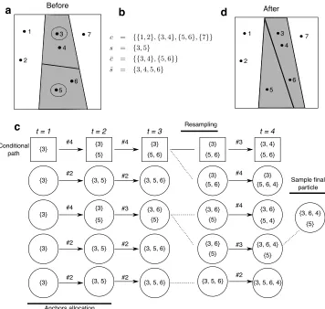
Figure 1: (a) Example illustrating the setup of a split merge and (b) the notation used in Section 3.1. The seven points denote the observation indices. While we show points in a two-dimensional space for visualization, the methodology does not rely on any topological properties of the observation space. The dashed circles denote the anchors s, and the shaded region, the closure of the anchors. (c) Example of a single PGSM step with σ = (3,5,6,4). Square boxes represent particles corresponding to the fixed conditional path. Circles represent regular particles. Each particle has an associated clustering denoted by the set or pair of sets written inside each particle. Arrows indicate proposal draws labelled by the proposed state (see Figure 2). Dashed lines indicate when resampling occurs. (d) Configuration after the PGSM update illustrated in c.

initially clustered with the anchor points. The anchor proposal distribution h obviously impacts the performance of this procedure. We empirically compare the performance of three anchor proposal distributions h in Section 4.3.

Proposition 1 If c∼π, whereπ is given by Equation (4), then the output of Algorithm 1,

c0, satisfiesc0 ∼π. That is, the Markov kernelK(c0|c)induced by Algorithm 1 isπ-invariant.

3.2 Overview of the particle Gibbs algorithm

Ideally, we would like to sample independently from π in Algorithm 1, that is we would like to have K(c0|c) = π(c0), but this is too computationally expensive if |s| is large. Our primary contribution is an original way to address this issue using SMC-based methods.

In principle, it would be possible to use SMC methods to obtain a sample approximately distributed according toπ (Fearnhead, 2004). However, if we were to use this sample within Algorithm 1, the resulting invariant distribution would not beπ. For this reason, we consider Particle MCMC (PMCMC) methods (Andrieu et al., 2009, 2010).

PMCMC methods allow us to use SMC ideas in a principled way within MCMC schemes. We will focus here on the PG sampler and show how one can use this methodology to obtain an efficient MCMC kernel K targeting the distribution π given in Equation (5). The outcome of the PG sampling steps will be either to cluster all the points insinto one block or to breaksinto two clusters, with the restriction that each of the two blocks should contain one anchor. Interestingly, the form of the PG algorithm is the same no matter if the two anchors were previously together or apart before its execution. This contrasts with previous split-merge algorithms such as Jain and Neal (2004), which require a different treatment for split and merge moves.

To sample from π, PG breaks the sampling of c0 into a sequence of n := |s| simpler sampling problems. In this scenario, contrary to most applications of PG, there is no intrinsic time ordering of the observations. We randomize the order in which the points are included by introducing, conditionally onsands, a random permutationσ := (σ1, . . . , σn). This permutation is sampled using Algorithm 2.

Algorithm 2

1: function SamplePermutation(s, s)

2: σ1∼Uniform(s)

3: σ2←s\{σ1}

4: (σ3, σ4, . . . , σn)←UniformPermutation(s\s)

5: return σ

6: end function

In other words, σ is uniform over the permutations of the observation indices in ssuch that the members of s appear in the first two entries. The variable σt specifies the index of the observation yσt introduced into the PG algorithm at SMC iteration (“algorithmic” time)tandxtis the corresponding allocation decision. A particlextis defined as a sequence of allocation decisions, xt:= (x1, . . . , xt), where xt∈ X,t∈ {1, . . . , n}.

Givenσ, we denote the SMC proposals used within PG byqσ_t(xt|xt−1), and the

interme-diate unnormalized target distributions, byγσ_t(xt). We remind the reader that bothγtσ and

unnormalized target distributions. For our methodology to provide consistent estimates, only the following weak assumptions have to be satisfied.

Assumption 1 For all t ∈ {1, . . . , n}, we assume support(γ_tσ) ⊆ support(qσ_t) where

q_tσ(xt) :=q1σ(x1)Qt_k=2q_kσ(xk|xk−1) for t≥2.

Assumption 2 We assume that there exists a bijection φσ _{taking a particle as input, and}

outputting a clustering ofs. More precisely,φσis a bijection between the support of the

pro-posal, and the support of the split-merge target distribution,φσ: support(q_nσ)→support(π).

Assumption 3 We assume thatγ_nσ(xn)∝π(φσ(xn)).

Assumption 1 ensures that all the importance weights appearing in the SMC method are well-defined. Assumption 2 is a simple condition ensuring that we can consistently relabel the particles. Assumption 3 ensures that we target the desired distribution at algorithmic timen. Note that Assumption 3 only restricts the choice ofγt for the final SMC iteration,

t=n. We use this flexibility in Section 3.4. We show in the next section how to designqσ_,

γσ,φσ and X that satisfy these assumptions.

PG proceeds in a way similar to standard SMC algorithms, with the important difference that one of theN particle paths is fixed. In our setup, this path is obtained using the inverse of the bijection described in Assumption 2, applied to the state of the restricted clustering

c prior to the current PG step. As discussed in Chopin and Singh (2015), we can without loss of generality set the genealogy of the conditioning path c to (1, ...,1), i.e. we use the particle index p = 1 for this conditioning path: x1_n := (φσ)−1(c). This defines a path by taking a prefix of length tof the vectorx1

n forx1t, i.e. x1t = x1n

1:t.

The final ingredient required to describe the PG algorithm is a conditional resampling

distribution r(a | w), where a := (a2, . . . , aN) denotes the resampling ancestors, ap ∈ {1, . . . , N}, and w:= (w1, . . . , wN) denotes a vector of probabilities. We limit ourselves to multinomial resampling:

r(a|w) = N

Y

p=2

r(ap|w) = N

Y

p=2

wap_{. (6)}

More elaborate schemes can be used, see Andrieu et al. (2009, 2010). Instead of resampling at each time step as in vanilla SMC algorithms, we only resample when the relative Effective Sampling Size (ESS) criterion, which takes values between 0 and 1, is below a pre-specified thresholdβ,β ∈[0,1]. The adaptive resampling procedure was proposed by Liu and Chen (1995) for standard particle methods and the correctness of this procedure for PG has been established in Lee (2011). The resulting procedure is described in Algorithm 3.

Algorithm 3

1: function ParticleGibbsSplitMerge(s, s, c,π) . Inputs coming from Algorithm 1

2: σ ←_{SamplePermutation}(s, s)

3: x1_n←(φσ)−1(c) . Compute the conditional path

4: for t∈ {1, . . . , n−1} do

5: x1_t ← x1_n1:t . First particle of each generation matches the conditional path

6: end for

7: for p∈ {2, . . . , N}do .Initialize particles

8: xp₁ ∼qσ₁ (·) 9: xp₁ ←(xp₁)

10: end for

11: for p∈ {1, . . . , N}do . Initialize incremental importance weights 12: w˜p₁ ← γ1σ(x

p

1) qσ

1(x

p

1)

13: end for

14: for p∈ {1, . . . , N}do

15: wp₁ ← w˜

p

1

(PN_p0₌₁w˜p 0 1 )

. Compute normalized weights

16: end for

17: for t∈ {2, . . . , n} do

18: if (NPN

p=1(w

p

t−1)2)−1 < β then . Resample only if relative ESS is too low

19: a∼r(· |wt−1) . Perform the conditional resampling step

20: w˜t−1 ←(1,1,1, . . . ,1) .Reset the weights

21: else

22: a←(1,2,3, . . . , N) . Resampling is skipped: setato the identity map

23: end if

24: forp∈ {2, . . . , N} do 25: xp_t ∼q_tσ · |xap

t−1

.Propose new block allocation for yσt 26: xp_t ←(xap

t−1, x

p

t) . Concatenate new block allocation to path

27: end for

28: forp∈ {1, . . . , N} do 29: w˜_tp←w˜_tp₋₁·w(xap

t−1, x

p

t) .Update weights (see Equation (9))

30: end for

31: forp∈ {1, . . . , N} do 32: w_tp← w˜pt

(PN_p0₌₁w˜p 0

t )

.Compute normalized weights

33: end for

34: end for

35: x0_n∼PN

p=1w

p

nδxpn(·) .Sample particle representing new state

36: c0 ←φσ(x0_n) . Compute updated partition

37: return c0

38: end function

all points insinto one block (i.e. when|φσ(x0_n)|= 1), and others, to various way of splitting

{{σ1}} {σ1}

{{σ₁},{σ₂}} {σ1} {{σ1,σ2}}

{σ1,σ2}

{{σ1},{σ2}} {σ₂} #1

#2

#3

#4

Merge Initialize Split

S(#1) := {#2,#4}

S(#2) := {#2}

S(#3) := {#3,#4} S(#4) := {#3,#4}

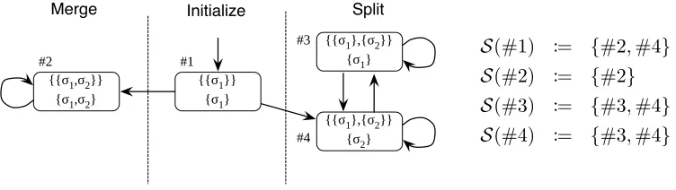
Figure 2: Left: State spaceX and allowed transitionsS(·) for the local allocation decisions. Right: allowed transitions between the states.

Correctness of this procedure follows straightforwardly from the original PG argument (see Appendix B for details):

Proposition 2 Under Assumptions 1, 2, and 3, the output of Algorithm 3, c0, satisfies

c0 ∼π if c∼ π, for any N ≥2, i.e. the Markov kernel K(c0|c) induced by Algorithm 3 is

π-invariant.

3.3 Intermediate target distributions and proposals construction

We detail here the construction of a set of proposal distributions qσ, unnormalized target distributions γσ, and mappings φσ satisfying Assumptions 1 to 3. We denote the space of possible allocation decisions at a given PG iteration by X. Our construction is based on an encoding where the space X consists in the rectangles shown in Figure 2. We call the rectangles states for short. These states are used to build particles: recall that a particle xt is defined as a list of local decisions,xt:= (x1, . . . , xt), xt0 ∈ X.

The state appended to a particle at time trepresents (a) the clustering restricted to the anchors (shown in the first line of each rectangle in Figure 2), and (b), the cluster joined by yσt (encoded by the anchor(s) contained in the joined cluster, second line in the same figure). As shown in Figure 2, the “merge state” (left) is an absorbing state, encoding the fact that following this local decision, all children particles are forced to join the unique block in the restricted clustering. The two “split states” (right), on the other hand, both have two outgoing transitions, encoding the fact that for each index in s\s, the corresponding observation needs to be allocated to one of the two blocks.

There is a bijection between the support of π, and particles respecting the transition constraints defined by the arrows in Figure 2. More precisely, for each statex∈ X, we let S(x) denote the set of allowed transitions fromx. We writext∈ Stif (a)x1 = #1, and (b)

for all t0 ∈ {2, . . . , t}, xt0 ∈ S(x_t0₋₁). From this definition, we obtain the following result

Proposition 3 For any permutation σ satisfying {σ1, σ2}=s, there is a bijective mapφσ

from the space of particles respecting the transition constraints, Sn, to the support of the

restricted target, support(π).

We use this bijection to define a sequence of intermediate target and proposal distribu-tions. The intermediate target at time tof supportS_t is given by:

γ_tσ(xt) :=τ1(ct)



 Y

b∈ct

τ2(|b|)L(yb)



, (7)

where ct = φσ1:t(xt). By construction, we have that for t = n, γnσ(xn) ∝ π(φσ(xn)) so Assumption 3 is satisfied.

We define as proposals:

q₁σ(x1) := δ#1(x1), (8)

qσ_t(xt|xt−1) :=

γ_tσ(xt)

P

x0t∈S(xt−1)γ

σ

t (xt−1, x0t)

,

where (xt−1, x0t) denotes the concatenation of x0t to the vector xt−1, and xt = (xt−1, xt). These definitions satisfy Assumption 1, and yield the following weight updates:

wt(xt−1, xt) :=

γ_tσ(xt)

γ_tσ₋₁(xt−1)

1

qσ_t(xt|xt−1)

(9)

=

P

x0

t∈S(xt−1)γ

σ

t (xt−1, x0t)

γσ

t−1(xt−1)

= X

x0t∈S(xt−1)

γ_tσ(xt−1, x0t)

γσ

t−1(xt−1) .

Ift >|s|then Equation (10) simplifies as follows

γ_tσ(xt)

γ_tσ₋₁(xt−1)

= τ2(|b

+

t |)

τ2(|b−t |)

L

y_b+

t |yb

−

t

, (10)

where

Ly_b+

t |yb

−

t

:=

Ly_b+

t

Ly_b−

t

. (11)

Hereb−_t andb+_t encode the block in which a point is added to when transitioning from xt−1

to xt, the first being the block before the addition, and the second, the same block after the addition:

b−_t :=ct−1\ct, b+t :=b −_{∪ {}

σt}. (12)

3.4 An improved sequence of intermediate target distributions

We now describe an improvement over the basic intermediate and proposal distributions presented in the previous section. This improvement addresses a “greediness” problem of the (conditional) SMC procedure. Consider a case where the ratioτ1(1)/τ1(2) between a merge

and a split is large. This can occur for example when the Dirichlet process concentration parameterα0 is small. In this case, the proposal in the first non-trivial step,qσ2, will assign

most of its mass to the transition from state #1 to state #2 (see Figure 2). However, the likelihood might overcome this prior when |s| is large. But proposing such split has low probability under the definitions given in the previous section, as #2 is an absorbing state. To overcome this issue, we build a new sequence of intermediate distributions, which delay the incorporation of the prior:

c

γσ_t(xt) :=

(

1[xt∈ St], ift∈ {1,2}, (γ₂σ(x1:2))ζt γ

σ t(xt) γσ

2(x1:2), otherwise.

(13)

whereζt is a positive increasing annealing schedule such that ζn= 1. We use the following proposal based on these new intermediate distributions:

c

q₁σ(x1) := δ#1(x1), (14)

c

qσ_t(xt|xt−1) :=

c

γ_tσ(xt)

P

x0

t∈S(xt−1)γc

σ

t (xt−1, x0t−1) .

This yields the weight updates:

c

wt(xt−1, xt) :=

X

x0_t∈S(xt−1)

c

γ_tσ(xt−1, x0t)

d

γσ

t−1(xt−1)

. (15)

For simplicity, we pickζt = _nt−−22. This choice simplifies ratios of intermediate distributions

to:

c

γ_tσ(xt)

d

γσ

t−1(xt−1)

=

(

1 ift= 2,

(γ₂σ(x1:2))∆ζ γ

σ t(xt) γσ

t−1(xt−1) ift >2,

(16)

where ∆ζ := (n−2)−1. 3.5 Runtime analysis

To simplify the analysis of the running time, we make a few assumptions.

Assumption 4 The parametric likelihood model has the following properties:

1. letψ:=ψ(yb)denote a sufficient statistic, and define, with a slight abuse of notation,

L(ψ) := L(yb). For a given sufficient statistic value ψ, the likelihood L(ψ) can be

computed in time O(l),

2. the sufficient statistic for b+, ψ+ := ψ(yb+), can be updated in time O(u) from the

The next assumption holds for all the clustering priors reviewed in Section 2.

Assumption 5 The ratio τ2(j+1)

τ2(j) can be computed in constant time.

For example, with a Dirichlet process, this ratio is equal to j!/(j−1)! =j. Since |b+|= |b−|+ 1, Assumption 5 implies that the ratio τ2(|b+|)

τ2(|b−|) in Equation (10) can be computed in

constant time.

Proposition 4 Under Assumptions 4 and 5, one weight computation, Equation (15), takes

time O(u+l). The storage cost per particle isO(1). Moreover, the running time per weight

computation is independent of the number of clusters.

The running time result follows directly from the fact that|S(·)| ≤2, and hence the sum in Equation (15) has a constant number of terms. The constant storage cost follows from the finite dimensionality of the sufficient statistics (see Assumption 4), and from |X |= 4.

We also remind the reader that for most resampling schemes, including the one in Equation (6), the computational cost as a function of the number of particles and SMC iterations isO(N n) =O(N|s|) (Doucet and Johansen, 2011).

3.6 Generalization

For simplicity, we have assumed so far that |s|= 2, and hence, according to the auxiliary variable analysis of Appendix B, |c| ≤ 2. In fact, the same auxiliary variables with more than two anchor points can be used to construct novel sampling algorithms. Details are given in Appendix D.

This generalization loses some interpretability compared to the split-merge case (|s|= 2), but can be useful in finite clustering models. In this case, it may only be possible to split a cluster if a merge is performed simultaneously. For this reason, we use |s| = 3 in the finite Dirichlet mixture model examples in Section 4.3. For the Dirichlet Process, we did not observe notable improvements by going from |s|= 2 to |s| = 3, so we use the former setting for the non-parametric models.

4. Applications

In this section, we demonstrate the performance of our methodology and compare it to standard alternatives. We use a series of synthetic datasets covering a large spectrum of cluster separateness, as well as real data coming from a geolocation application.

4.1 Implementation and evaluation

We have implemented the following three Dirichlet Process (DP) clustering samplers in the same Python codebase: the PGSM method described in this work, the efficient Sequentially-Allocated Merge Split (SAMS) method of Dahl (2003), as well as the standard Gibbs sampler. The code and instructions allowing to reproduce the experiments is available

at https://github.com/aroth85/pgsm. The implementation of the likelihood

the correctness of our computer implementations by computing the true posterior distribu-tion on small examples via combinatorial enumeradistribu-tion, and verified that the Monte Carlo estimates converged to this distribution for all three methods.

Unless we state otherwise, we initialized the samplers with the single-cluster configu-ration. In datasets much smaller than those studied in this work, initializing the Gibbs sampler to the fully disconnected clustering is advantageous (Sudderth, 2006), but in larger datasets, the quadratic burn-in cost involved with this initialization is not scalable. How-ever, we verified that after a long burn-in period the Gibbs method initialized to the fully disconnected clustering eventually reaches the same likelihood values in the synthetic exam-ples. We also investigate the high cost of the fully disconnected initialization in the results shown in Figure 9.

To evaluate the performance of the samplers, we held-out a random but fixed 10% of each dataset. We collected samples and computed the predictive likelihood and V-measure (Rosenberg and Hirschberg, 2007) every 100 iterations. All experiments are replicated 10 times, and smoothed using a moving average with a window size of 20 for plotting.

4.2 Likelihoods and priors

In six of the synthetic experiments and the geolocation experiments discussed further in Section 4.3 and Section 4.4, we used a Normal-Inverse-Wishart conjugate likelihood model. In two of the synthetic experiments in Section 4.3 we used Bernoulli mixture models with 50 dimensions. Each dimension is an independent draw from a Bernoulli random variable with cluster specific parameters. We set a proportion of the dimensions to be uninformative as follows. Values for uninformative dimensions were drawn from Bernoulli variables with parameter 0.5 regardless of the cluster membership. Values for the remaining dimensions were drawn from cluster specific Bernoulli variables with parameters sampled from the Uniform distribution. For the cancer data discussed in Section 4.5, we use the application-specific PyClone likelihood model (Roth et al., 2014). The PyClone model uses genomic sequence data from tumours to identify mutations which co-occur in cells and estimates the proportion of cells harbouring the mutations. The model is not conjugate, so we apply a discretization that allows us to treat the model as conjugate. Complete details for each model are provided in Appendix E.

We use a DP prior with base measure given by the conjugate prior of the corresponding likelihood model in all experiments. We use a Gamma(1,0.1) prior and resample the value of the concentration parameters α0 using a standard auxiliary variable method (Escobar

and West, 1995). The value of α0 is initialized to 1.0.

4.3 Artificial datasets

10

₁₀

1400

1300

1200

1100

1000

900

800

700

Predictive log likelihood

a

10

₁₀

0.0

0.2

0.4

0.6

0.8

1.0

V-measure

b

5

10

20

100

10

₁₀

c

10

₁₀

d

Cluster informed

Threshold

Uniform

10

₁₀

e

10

₁₀

CPU time (seconds, log scale)

f

Never

0.25

0.5

0.75

Always

Figure 3: Effect on the predictive performance and clustering accuracy as a function of CPU time in log scale. a) and b) Varying the number of particles with the cluster informed proposal and a relative ESS resampling threshold of 0.5. c) and d) Varying the distribution for proposing pairs of anchor points,h, with 20 particles and an ESS resampling threshold of 0.5. e) and f) Varying the relative ESS resampling threshold with the cluster informed anchor proposal and 20 particles.

to be uninformative. Finally, we used 64 (DIM064) and 128 (DIM128) dimensional Normal datasets from Fr¨anti et al. (2006) with 1024 data points and 16 clusters.

We started with a series of pilot experiments on S1 only, designed to assess the effect of various tuning parameters on the performance of PGSM. For all pilot experiments we use the unmixed PGSM sampler to isolate the effect of each tuning parameter. In practice it is usually better to alternate between one iteration of the PGSM sampler and one iteration of the Gibbs sampler. The effect of this mixing is explored later in this section.

10

₁₀

-166

-165

-164

-163

-162

-161

Predictive log likelihood

(

×

10

4

)

a

Ber­0.5

10

₁₀

0.0

0.2

0.4

0.6

0.8

1.0

V-measure

b

10

₁₀

-320

-300

-280

-260

-240

-220

c

DIM128

10

₁₀

0.0

0.2

0.4

0.6

0.8

1.0

CPU time (seconds, log scale)

d

Cluster informed

Threshold

Uniform

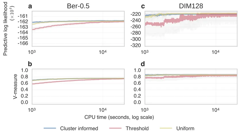
Figure 4: Effect on the predictive performance and clustering accuracy as a function of CPU time in log scale with different distributionhfor proposing pairs of anchor points. a) andb) Comparison using a 50 dimensional Bernoulli dataset with 50% of the dimensions being uninformative. c) and d) Comparison using a 128 dimensional Normal dataset.

the initial iterations. The performance difference are negligible and the PGSM sampler generally seems insensitive to the number of particles for this dataset. For subsequent experiments we used 20 particles.

Next we compare the performance of different proposal distributions for the anchor auxiliary variables (Figures 3candd). For this experiment we kept the number of particles fixed at 20 and the resampling threshold at 0.5. We consider three proposal distributions.

Uniform: Sample the anchors uniformly at random from the T₂ possibilities.

Cluster informed: Sample the first anchor uniformly at random. Sample a cluster to draw the second anchor from with probability _|c−1_1| for the cluster containing the first anchor; otherwise proportional to

L(y¯_b∪b) L(y¯_b)L(yb)

where ¯bis the cluster containing the first anchor andbis the candidate cluster. Sample the second anchor uniformly from the chosen cluster.

To ensure the adaptation of the informed proposals stops, and does not perturb the invariant distribution of the sampler, we only update the proposal distributions when the number of clusters instantiated breaks the previous record. Adaptation is guaranteed to terminate in finite time given there are only a finite number of points. This would usually take a long time, so in practice it is advantageous to stop adaptation after a fixed period of time. Detailed implementations of the cluster informed and threshold informed proposals are given in Appendix F. Our results suggest that performance is not strongly affected by the anchor proposal distribution h. We only saw a small advantage when using the informed proposal distributions for the auxiliary anchor variables ins. We also explored the effect of

h in higher dimensional datasets (Figure 4). Again we found the results are not sensitive to the choice of h. With the exception of the circle dataset, where we used the uniform proposal, we used the cluster informed prior for both the PGSM and SAMS samplers in subsequent experiments.

The frequency of the resampling step had a larger effect. A critical implementation point in order for the PGSM method to work is that resampling should be done adaptively by monitoring the ESS of the particle approximations in Algorithm 3 (Liu and Chen, 1995; Lee, 2011). We varied the relative ESS resampling thresholdβ from 0 (never resample) to 1 (always resample) (Figures 3 e and f). We observed that the performance is markedly degraded if resampling is performed after each SMC iteration, but similar for all other resampling thresholds. We used a threshold of 0.5 in all other experiments.

Next, we used the dataset C1 to investigate the effectiveness of our method with the finite clustering model introduced in Section 2, with the number of clusters fixed tok0 = 5.

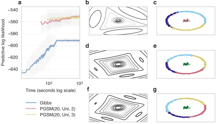
In this case, standard split-merge methods such as SAMS are less helpful since only merging can be performed when the maximum number of clusters has been allocated. The PGSM sampler does not have this restriction and naturally allows simultaneously splitting and merging while preserving the total number of clusters. Furthermore, the PGSM sampler can use more than two anchors, potentially allowing for large changes in configuration without altering the number of clusters. We compared the PGSM with two (|s| = 2) and three (|s| = 3) anchors to the Gibbs sampler. The PGSM method outperformed the Gibbs sampler, though increasing the number of anchors did not improve the performance (Figure 5 a). We plot the predictive densities (Figure 5 b, d, f) and cluster allocations (Figure 5 c, e, g) after running each sampler for 1000 seconds. At this point the PGSM sampler used a single cluster to model the points in the middle, while the Gibbs samplers used two clusters to model the central cluster.

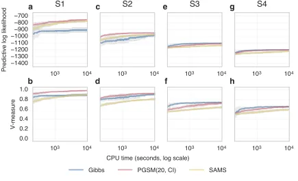
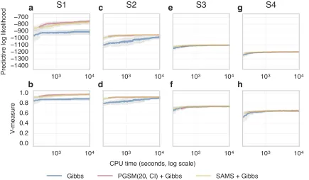
In Figures 6 and 7 we show a series of experiments on the four datasets S1–4 describe in the previous section. We compare the PGSM to standard Gibbs and the SAMS method of Dahl (2003). We first compared pure kernels, where the split-merge samplers are not mixed with standard Gibbs moves (Figure 6). The pure PGSM kernel outperformed both Gibbs and SAMS on datasets S1 and S2. The Gibbs kernel and PGSM perform similarly for datasets S3 and S4, and both outperformed SAMS. When the split-merge moves are mixed with standard Gibbs moves, the split-merge methods outperformed Gibbs on datasets S1 and S2, with all methods showing similar performance on datasets S3 and S4 (Figure 7).

b

c

d

e

f

g

10

₁₀

Time (seconds log scale)

640

620

600

580

560

540

Predictive log likelihood

a

Gibbs

PGSM(20, Uni, 2)

PGSM(20, Uni, 3)

Figure 5: Comparison of Gibbs and PGSM for finite Dirichlet prior with k0 = 5. a)

10

₁₀

1400

1300

1200

1100

1000

900

800

700

Predictive log likelihood

S1

a

10

₁₀

0.0

0.2

0.4

0.6

0.8

1.0

V-measure

b

10

10

S2

c

10

₁₀

d

10

10

S3

e

10

₁₀

f

10

10

S4

g

10

₁₀

CPU time (seconds, log scale)

h

Gibbs

PGSM(20, CI)

SAMS

Figure 6: Comparison of MCMC algorithm using only a single kernel at a time (pure ker-nels) on 2D Normal datasets. Predictive log likelihood for datasets a) S1;c) S2; e) S3;g) S4. V-measure for datasetsb) S1;d) S2;f) S3;h) S4.

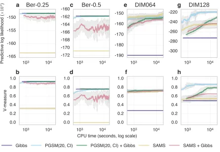
(Figures 8 a-d). The mixed SAMS sampler failed to reach the same predictive likelihood as the PGSM and Gibbs methods, oscillating around lower values. The unmixed SAMS sampler appears to be trapped in a local mode, corresponding to poor predictive likelihood and V-measure. For the Normal datasets, the Gibbs sampler was trapped in a local mode and had markedly worse performance than other methods (Figures 8 e-h). The unmixed samplers outperformed the mixed equivalents on the 64 dimensional data. Furthermore, the unmixed PGSM method had a large performance advantage over all other methods on the 128 dimensional dataset.

4.4 Geolocation data

10

₁₀

1400

1300

1200

1100

1000

900

800

700

Predictive log likelihood

S1

a

10

₁₀

0.0

0.2

0.4

0.6

0.8

1.0

V-measure

b

10

10

S2

c

10

₁₀

d

10

10

S3

e

10

₁₀

f

10

10

S4

g

10

₁₀

CPU time (seconds, log scale)

h

Gibbs

PGSM(20, CI) + Gibbs

SAMS + Gibbs

Figure 7: Comparison of MCMC algorithm using split-merge moves combined with stan-dard Gibbs moves (mixed kernels) on 2D Normal datasets. Predictive log likeli-hood for datasets a) S1; c) S2; e) S3; g) S4. V-measure for datasets b) S1; d) S2;f) S3;h) S4.

We use this data as a proxy for the estimation of mobile device user density. The DP mixture of Normal-Inverse-Wishart distributions provides a natural way to obtain a parsi-monious estimate of population density, where the flexibility on the shape and number of clusters can accommodate a broad range of density variability factors ranging from densely populated cities to vast low-density rural areas.

We summarize the results in Figure 9. In Figures 9a-c, we display quantitative results as measured by held-out predictive likelihood performance. In Figure 9 a, we show that mixed PGSM, mixed SAMS and Gibbs samplers perform similarly. In Figure 9b, we show that the performance of SAMS is considerably degraded if SAMS is not mixed with a Gibbs kernel. In Figure 9c, we show that the performance of PGSM is less degraded if not mixed with a Gibbs kernel.

10

₁₀

-165

-160

-155

-150

P

re

di

ct

iv

e

lo

g

lik

el

ih

oo

d

(

10

4

)

a

Ber­0.25

10

₁₀

0.0

0.2

0.4

0.6

0.8

1.0

V-measure

b

10

₁₀

-172

-170

-168

-166

-164

-162

-160

c

Ber­0.5

10

₁₀

0.0

0.2

0.4

0.6

0.8

1.0

d

10

₁₀

-190

-180

-170

-160

-150

e

DIM064

10

₁₀

0.0

0.2

0.4

0.6

0.8

1.0

f

10

₁₀

-300

-280

-260

-240

-220

g

DIM128

10

₁₀

0.0

0.2

0.4

0.6

0.8

1.0

CPU time (seconds, log scale)

h

Gibbs

PGSM(20, CI)

PGSM(20, CI) + Gibbs

SAMS

SAMS + Gibbs

Figure 8: Comparison of MCMC algorithm using split-merge moves with combined with standard Gibbs moves (mixed kernels) on 50 dimensional Bernoulli data with 25% (Ber-0.25) and 50% (Ber-0.5) and Normal data 64 (DIM064) and 128 (DIM128) dimensions. Predictive log likelihood for datasets a) Ber-0.25; c) Ber-0.5; e) DIM064;g) DIM128. V-measure for datasetsb) Ber-0.25;d) Ber-0.5;f) DIM064; h) DIM128.

initialized at the fully connected configuration for the same time (Figures g and h); the third, after running the Gibbs sampler for 105 seconds (Figuresiandj). This demonstrates that our method can produce accurate and compact density estimates without relying on an expensive initialization phase.

4.5 Inferring population structure in heterogeneous tumours

103 ₁₀4 ₁₀5 2400

2420 2440 2460 2480 2500 2520 2540

Predictive log likelihood

a

103 ₁₀4 ₁₀5

2000 2100 2200 2300 2400 2500 2600

b

103 ₁₀4 ₁₀5

2400 2420 2440 2460 2480 2500 2520 2540

CPU time (seconds, log scale)

c

Gibbs PGSM(20, CI) PGSM(20, CI) + Gibbs SAMS SAMS + Gibbs

d

e

f

g

h

i

j

Figure 9: Geolocation dataset. Comparison of predictive likelihoods of a) mixed kernels; b) PGSM pure and mixed kernels; c) SAMS pure and mixed kernels. d) MOPSI geolocation dataset. e) Predictive density of Gibbs initialized from the discon-nected configurations after one iteration;d) with point data points overlayed. g) and h) Predictive density of mixed PGSM kernel after an equivalent amount of time. i) and j) Predictive density of disconnected Gibbs after 105 seconds.

10

₁₀

5374

5372

5370

5368

5366

Predictive log likelihood

a

Gibbs

PGSM(20, CI)

PGSM(20, CI) + Gibbs

SAMS

SAMS + Gibbs

10

₁₀

0.56

0.58

0.60

0.62

0.64

V-measure

b

10

₁₀

5374

5372

5370

5368

5366

Predictive log likelihood

CPU time (seconds, log scale)

c

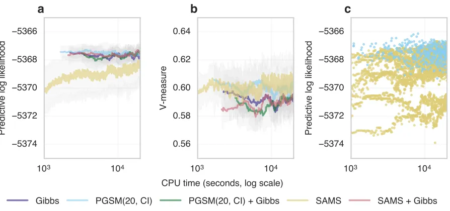
Figure 10: Clustering of cancer mutations from synthetic next-generation sequencing data. a) Comparison of predictive likelihood. b) Trace of log predictive likelihood for PGSM and SAMS pure kernels from 10 random restarts.

We show results on a dataset with 10,000 synthetic mutations in Figure 4.5. All methods except the pure SAMS kernel performed similarly in terms of predictive likelihood, while the pure SAMS kernel performed significantly worse (Figure 4.5 a). The pure PGSM and SAMS kernels outperformed the other methods in terms of V-measure, though the difference were small (Figures 4.5b).

As observed in the other domains, the performance of SAMS critically depends on mixing the kernel with GIBBS moves. We show the data points for each replication of the pure split-merge kernels further supporting this point (Figure 4.5 c).

5. Discussion

We have proposed a new methodology to design efficient split-merge moves for Bayesian mixture models. The method also generalizes to new types of moves useful for finite clus-tering models when |s| > 2. We have shown empirically that the proposed method is competitive in a range of clustering and likelihood models, including synthetic and real datasets from geolocation and genomics applications.

Another area of improvement comes from the development of resampling schemes tai-lored to discrete latent variables. In Algorithm 3, the number of possible distinct successors for each given particle is a small finite number (at most two if |s|= 2 for example). The complexity of the problem comes from the fact that a potentially long sequence of such decisions need to be made in order to split a cluster. In these specific scenarios, custom PMCMC methods based on the early work of Fearnhead and Clifford (2003) have been developed in Whiteley et al. (2010) and would provide futher improvement.

The fact that the state transitions S(·) have an absorbing state has both advantages and disadvantages. On the one hand it may cause Algorithm 3 to be greedy, as explained in Section 3.4. We have described in the same section a choice of intermediate and proposal distributions tailored to alleviate this issue. A potential alternative consists in designing a resampling distributionr, which conditions on the survival of at least one representative of both a merge and a split. None of the existing resampling schemes have this property. On the other hand, having an absorbing state has the advantage that if all particles simulated by Algorithm 3 at some iterationtare equal to the merge absorbing state (i.e. xp_t = #2 for all particle indexp∈ {1, . . . , N}), then there is no need to continue the computation of the particle filter fort0 > t.

In standard applications of the PG algorithm, coalescence of the particle genealogy may cause slow mixing as noted in Andrieu et al. (2010). The issue is that the particles x1_n,x2_n, . . . ,xN_n appearing in Algorithm 3 have components at timetfortnwhich coincide with high probability with the components of the conditioning path. This can be resolved using more sophisticated MCMC moves on the PG auxiliary variables (Whiteley, 2010; Whiteley et al., 2010; Lindsten et al., 2014). In our non-standard setup, this issue is partially mitigated by the fact that the order σ at which the particles are introduced is itself random. Nonetheless, it would be interesting to implement these more advanced schemes to the problem at hand.

We have shown in Section 4.5 a simple and effective method for handling models where each cluster component is governed by a non-conjugate model with a low-dimensional pa-rameterization. We leave for future work the extension of our method to higher dimensional non-conjugate likelihood models. This problem can be approached, for example, by com-bining our method with the auxiliary variables described in Neal (2000).

Acknowledgements

Alexandre Bouchard-Cˆot´e’s research was funded by an NSERC Discovery Grant. Arnaud Doucet’s research is partially supported by EPSRC grants EP/K000276/1 and EP/K009850/1. Andrew Roth was partially supported by a CIHR CGS scholarship. Computing was sup-ported by WestGrid and Compute Canada.

Appendix A. Correctness of the decomposition into split-merge subproblems

Examples of valid configurations for c' Examples of invalid configurations for c'

Figure 11: Assuming that the values of c, c− and sare as in Figure 1, this illustrates some examples of configurations c0 that are part of (left), or excluded from (right), the support ofc0|s, c−.

and c− consists of the blocks of the partition cthat do not contain anchor points:

c−:={b∈c:b∩s=∅}, (17)

These intuitively correspond to the blocks of the partition that are forced to stay unchanged in this split-merge step. We will view the split-merge step as a Gibbs step conditioning on

c−, s.

A slight subtlety is that conditioning on the auxiliary variables not only forces the blocks in c− to stay constant; it also forces the other blocks to each contain at least one of the anchors. See Figure 11 for an example. This leads to condition 2 in Lemma 5.

Lemma 5 Letc, c0denote two partitions of[T]. Lets⊆[T]. Definec−:={b∈c:s∩b=∅}

and c−0 :={b∈c0 :s∩b= ∅}. Then c− = c−0 if and only if the following two conditions

hold:

1. c∩c−=c0∩c−, and,

2. b∈c0\c− =⇒b∩s6=∅.

Proof (=⇒) Condition 1 holds trivially. For condition 2, suppose (a) c− = c−0, (b),

b∈c0\c−, but (c)b∩s=∅. By (b), b∈c0 and b /∈c−. This and (c) implies that b∈ c−0. But this contradicts (a), so condition 2 holds as well.

(⇐=) First, suppose b∈c−. By condition 1,b∈c−0. Therefore, c−⊆c−0.

Second, suppose b ∈ c−0. By the contrapositive of condition 2, b /∈ c0\c−. This point and c−0⊆c0 implies thatb∈c−.

We can now turn to the proof of Proposition 1. We copy its statement here for conve-nience:

Proposition 6 If c ∼ π, then the output of Algorithm 1, c0, satisfies c0 ∼ π; i.e. the

Proof Consider the model augmented with the auxiliary variables s and c− (see Fig-ure 12(a)), defined formally using the following auxiliary distribution:

˜

π(s, c−, c) :=π(c)h(s)1[c−=c−(s, c)], (18)

wherec−(s, c) :={b∈c:b∩s=∅}. Note that this auxiliary distribution admits the target distribution as a marginal:

X

s

X

c−

˜

π(s, c−, c) = π(c)

X

s

h(s)X c−

1[c−=c−(s, c)] (19)

= π(c)X s

h(s) =π(c),

where the sum overc− is over all sets of subsets of [T], and the sum oversis over all subsets of [T]. We used the fact that only onec− satisfiesc−(s, c) =c−, and thath is a probability mass function.

Next, we introduce three kernels with inputs and outputs denoted by:

c_7−→K1

(s, c−, c)7−→K2 (s, c−, c0)7−→K3 c0. (20)

These kernels play the following roles:

• K1 samples the auxiliary variables according to ˜π(s, c−|c), while keepingc fixed, • K2 performs a Metropolis-within-Gibbs step onctargeting the auxiliary distribution

˜

π,

• K3 deterministically projects the triplet back to the original space, retaining only the

clustering c.

Formally:

K1(s0, c−0, c0|c) := h(s0)1[c=c0]1[c−0 =c−(s, c)], (21)

K2(s0, c−0, c0|s, c−, c) := π˜(c0|s, c−)1[s0=s]1[c−0=c−],

K3(c0|s, c−, c) := 1[c0 =c].

Since ˜π admits π as a marginal, the composition ofK1, K2,and K3 is clearly π-invariant.

It is therefore enough to show that when c− =c−(s, c) where c is a valid partition of [T], sampling from K2 is equivalent to sampling from the Markov kernel K(c0|c) induced by

Algorithm 1:

˜

π(c0 |s, c−) ∝ π(c0)1[c− =c−(s, c0)] (22) = π(c0)1[c−(s, c) =c−(s, c0)]

= τ1(|c0|) Y

b∈c0

τ2(|b|)L(yb)

!

1[c−(s, c) =c−(s, c0)].

Using Lemma 5, we now rewrite the support as follows:

s

c

-c

(a)

σ

g

c

(b)

Figure 12: Graphical models of the auxiliary variables used in the correctness proofs. The structure of the dependencies give an intuitive justification that the original model can be recovered as a marginal in both cases, as there are not directed path from the auxiliary variables to the original variables. (a) In Appendix A, the auxiliary variables aresandc−, and the original variable isc. (b) In Appendix B, the auxiliary variables areσ andg, and the original variable isc.

Let nowc0 =c0\c−. Plugging in the last line of Equation (22), we obtain:

˜

π(c0 |s, c−) = τ1(|c0|) 

 Y

b∈c0

τ2(|b|)L(yb)



1[c∩c−=c

0_{∩c−]1[b∩s6=∅] (24)}

= π(c0)1[c∩c− =c0∩c−],

whereπ(c0) is defined in Equation (5). Since Algorithm 1 does not change the clustering of points outside ofs(line 6 of Algorithm 1), it follows that the indicator function in the last line of Equation (24) is equal to one.

Appendix B. Correctness of particle Gibbs for split merge

We provide here the proof of Proposition 2. The main steps in the proof follow a structure similar to the proof of Proposition 1.

Proposition 7 Under Assumption 1, 2, and 3, and if c ∼ π, then the output of

Algo-rithm 3, c0, satisfies c0 ∼ π for any N ≥ 2; i.e. the Markov kernel K(c0|c) induced by

Algorithm 3 is π-invariant.

Proof We augment the modelc with the auxiliary variables σ and g (see Figure 12(b)), defined as:

1. σ is distributed according to the output of Algorithm 2, defined in Section 3.2.

2. Given σ and c, the variables g = (a2:n,x1:1:Nn, k) are distributed according to the specification of Algorithm 3, with the exception that all particle indices are shuffled according to an independent permutation of{1, . . . , N} at each generation. Herekis the index of the particle sampled at iterationn (on line (35)).

Next, we introduce three kernels with inputs and outputs denoted by:

These kernels play the following roles:

• K1 samples the permutationσ while keeping the auxiliary variablescfixed,

• K2 samplesgusing the PG step then sets c0 toφσ(xkn),

• K3 deterministically projects the triplet back to the original space, retaining only the

restricted clustering c0.

The kernel K2 is equivalent to a standard PG algorithm. Assumption 1, 3, and

The-orem 5(a) of Andrieu et al. (2010) imply that K2 is π-invariant (and in fact, irreducible).

Assumption 2 ensures that the computation of the conditioned path is well-defined.

Appendix C. Construction of the bijection

We provide here the proof of Proposition 3:

Proposition 8 For any permutation σ satisfying {σ1, σ2}=s, there is a bijective mapφσ

from the space of particles respecting the transition constraints, S_n, to the support of the

restricted target, support(π).

Proof Consider the following mapping:

φσ(xt) :=

{{σ1, . . . , σt}} ifxt∈ {#1,#2},

{σ1(xt), σ2(xt)} otherwise, (26) where σi(xt) :={σt0 :x_t0 = #(2 +i),1≤t0 ≤t}. It is easy to check that it has an inverse

given by:

(φσ)−1(c)

t:=

   

  

#1 ift= 1,

#2 ift >1,|c|= 1,

#3 ift >1,|c|>1, σ1∼cσt, #4 ift >1,|c|>1, σ2∼cσt,

(27)

where σi∼cσj means that yσi is in the same block as yσj for the clustering c. By the construction of the support of π, exactly one of the four cases above holds when c ∈ support(π).

Appendix D. Generalization to |s|>2

We describe here the algorithmic implications of increasing the number of anchor points, |s|, to some constant greater than two. This constant should be selected so that the number of partitions of |s|points is much lower than the number of particles.

The algorithm is generally unchanged, with the following exceptions:

2. as before, the local allocation state space X can be viewed as a pair each containing a partition and a block in this partition (see Figure 2). In the case where|s|= 2, the partitions are taken from the union of the set of partitions of a set of size one with the set of partitions of a set of size two. When|s|>2, we add more states, corresponding to partitions of a set of size three, etc. until we add states corresponding to partitions of a set of size|s|. The support of the transitionS consists in (a) edgesx→x0linking a state x0 such that removing one element from one of its blocks yields x, and (b) edges x → x0 where x and x0 correspond to the same partition of a set of size |s|. This is a generalization of the case |s| = 2 shown in Figure 2. The mapping φσ is generalized in the obvious way,

3. in Section 3.4 the following equations are substituted,

(a) t∈ {1,2} →t∈ {1,2, . . . ,|s|},

(b) t= 2→t∈ {2, . . . ,|s|},

(c) t >2→t >|s|,

(d) ∆ζ:= (n−2)−1→∆ζ := (n− |s|)−1_. Appendix E. Models

E.1 Multivariate normal

The first likelihood we use is the multivariate normal (MVN) with density denotedN(y|µ,Σ). We specify a normal inverse Wishart (NIW) prior for the mean and covariance parameters with density denoted NIW(µ,Σ|ν, r, u, S). The densities are given by

NIW(µ,Σ|ν, r, u, S) = N

µ|u,1 rΣ

IW(Σ|ν, S), (28)

N(y|µ,Σ) = 1 (2π)D2|Σ|

1 2

exp

−1

2(y−µ)

T_Σ−1_(y−µ)

,

IW(Σ|ν, S) = |S| ν

2

2νp2 Γ_D ν

2 |Σ|

−ν+p₂+1_exp

−1 2tr(SΣ

−1₎

,

where ΓD(x) =π D(D−1)

4 QD

d=1Γ x+d

−1 2

.

We use the following priors for all experiments (ν, r, u, S) = (ν0, r0, u0, S0) = (2 + D,1,0,I), where0is theDdimensional vector of zeros, andI is theDdimensional identity matrix. The posterior distribution ofµ,Σ giveny= (y1, . . . , ym) isN IW(µ,Σ|νm, rm, um, Sm) where

νm = ν0+m, (29)

rm = r0+m, um =

r0u0+Pm_i=1yi

rm

,

Sm = S0+

m

X

i=1

For computational efficiency it is convenient to express these updates iteratively using the following equations:

νm = νm−1+ 1, (30)

rm = rm−1+ 1, um =

rm−1um−1+ym

rm

,

Sm = Sm−1+ rm

rm−1

(ym−um)(ym−um)T.

Using these equations the Cholesky decomposition ofS0can be performed once using O(D3)

operations and cached. This decomposition can then be updated usingmrank one updates, each requiring O(D2) operations, to obtain Sm. This allows for efficient evaluation of the marginal and predictive likelihoods as|Sm|can be evaluated using O(D) operations using the Cholesky decomposition, instead of the standardO(D3) operations.

The marginal likelihood for the MVN-NIW congugate pair is

L(y) =

Z m

Y

i=1

L(yi|θ)H(dθ) (31)

=

Z m

Y

i=1

N(yi|µ,Σ)NIW(µ,Σ|ν, r, u, S) dµdΣ

= 1

πmD2

r D 2 0 r D 2 m

|S0|

ν0 2

|Sm| νm

2

QD

d=1Γ νm+d

−1 2

QD

d=1Γ

ν0+d−1

2 .

The predictive likelihood is given by

L(y+|y−) = L(y1, . . . , ym)

L(y1, . . . , ym−1)

(32)

= 1

πD2

r

D

2 m−1 r

D

2 m

|Sm−1|

νm−1 2

|Sm| νm

2

QD

d=1Γ νm+d

−1 2

QD

d=1Γ

νm−1+d−1

2 .

E.2 Bernoulli

We use a Bernoulli likelihood, Bernoulli(x|θ), with a Beta prior distribution, Beta(θ|α, β). We use the following priors (α, β) = (α0, β0) = (1,1) for all experiments. The densities are

Bernoulli(x|θ) = θx(1−θ)1−x, (33)

Beta(θ|α, β) = Γ(α)Γ(β) Γ(α+β)θ

The posterior density ofθgiveny= (y1, . . . , ym) is Beta(αm, βm) whereαm =α0+Pmi=1yi and βm =β0+Pm_i=1(1−yi). The marginal likelihood is

L(y) =

Z m

Y

i=1

L(yi|θ)H(dθ) (34)

=

Z m

Y

i=1

Bernoulli(yi|θ)Beta(θ|α0, β0) dθ

= Γ(α)Γ(β) Γ(αm)Γ(βm)

Γ(αm+βm) Γ(α0+β0)

,

and the predictive log likelihood is

L(y+|y−) = L(y1, . . . , ym)

L(y1, . . . , ym−1)

(35)

= Γ(αm−1)Γ(βm−1) Γ(αm)Γ(βm)

Γ(αm+βm) Γ(αm−1+βm−1)

.

E.3 PyClone

For the cancer genomics data we use the application-specific PyClone likelihood model over clonal prevalences, genotypes, and observed read counts. The key variables in the model are as follows (see Roth et al. (2014) for a more detailed description of the model):

φi : proportion of cancer cells with mutationi,φi ∈[0,1],

t : proportion of cancer cells in a sample (treated as known),t∈[0,1],

ψi : genotype of normal, non-mutated cancer and mutated cancer cells, ψi ∈(gN, gR, gV),

gx ∈ G={A,B,AA,AB, . . .},

πi,ψi : probability that mutationihas genotype ψi (elicited from auxillary data),

c(gx) = #A(gx) + #B(gx),

µ(gx) =

#A(gx)

c(gx)

,

ξ(ψ, φ, t) : probability of sampling a B from the population of cells in the sample, i.e.:

= (1−t)c(gN)µ(gN) +t(1−φ)c(gR)µ(gR) +tφc(gV)µ(gV) (1−t)c(gN) +t(1−φ)c(gR) +tφc(gV)

,

yi : number of sequence reads with a B and total number of reads covering mutationi, i.e.:

= (yi,b, yi,d)∈N2.

The generative model is specified as follow:

H0 = Uniform([0,1]), (36)

α0 ∼ Gamma(α0|a, b), H|α0, H0 ∼ DP(H|α0, H0),

φi|H ∼ H,

This model is not conjugate. However, if we letx∈ {x0, . . . , xM}=

n

0,_M1₋₁, . . . ,M_M−₋2₁,1

o

be a discretization of the interval [0,1] and replace the continuous uniform base measure,

H0 = Uniform([0,1]), with the discrete uniform measure, H0 = Uniform({x0, . . . , xM}), then we can approximate the model. Using this approximation, we can now treat the model as if it were conjugate. The marginal likelihood for data (y1, ..., ym) is given by

Z m

Y

i=1

L(yi|θ)H(dθ) =

Z m

Y

i=1 X

ψi∈G3

πi,ψiBinomial(yi,b|yi,d, ξ(ψi, φ, t))H(dφ) (37)

= M X k=0 m Y i=1 X

ψi∈G3

πi,ψiBinomial(yi,b|yi,d, ξ(ψi, xk, t)) 1 M = M X k=0 m Y i=1 exp        log X

ψi∈G3

πi,ψiBinomial(yi,b|yi,d, ξ(ψi, xk, t))

| {z }

Ξk(yi)

       1 M = M X k=0 exp m X i=1

Ξk(yi)

!

1

M,

where we have the sufficient statistics

Ξ(yi) = (Ξ0(yi), . . . ,ΞM(yi)). (38)

Remark 9 The possibly infinite sum P

ψi∈G3 is truncated to a finite sum over biologically

plausible states.

Appendix F. Anchor proposal distribution

The anchor proposal distribution, h, is a free tuning parameter for the PGSM sampler. In principle, proposals which are informed by the current clustering state of the chain or by the topology of the space may improve the performance of the sampler.

We consider two informed proposal distributions. While bespoke proposals for each model may perform better, we restrict attention here to proposals which can be applied generically to any class of model for which the PGSM sampler is applicable. In particular, we do not assume a distance metric is available. Both proposals we discuss are only applicable when two anchor points are used.

Algorithm 4 Cluster informed (CI) proposal 1: i1 ∼Uniform([T])

2: ¯b←b∈c s.t. i1∈b

3: c0 ←c\ {¯b} 4: forb∈c0 do 5: sb ← _LL_(y(_¯y¯b∪b)

b)L(yb) 6: end for

7: s¯_b ←

P b∈c0sb

|c|−1 .Merge probability is set to

1

|c|−1

8: forb∈c do 9: pb← Psb

b∈csb 10: end for

11: b0 ∼Discrete(c, pb) .Sample a blockb0 inc with probability pb 12: i2 ∼Uniform(b0\i1)

13: return i1, i2

Algorithm 5 Threshold informed (TI) proposal 1: i1 ∼Uniform([T])

2: forb∈c do 3: if i1 ∈b then

4: b←b\i1

5: end if

6: sb ←τ2(b)L(yi1|b) . CRP attachment probability where L(·|b) is the predictive

distribution 7: end for 8: forb∈c do 9: pb← Psb

b∈csb 10: end for

11: b0 ∼Uniform({b:pb ≥t}) . tis a pre-specified threshold, set to 0.01 in the experiments

12: i2 ∼Uniform(b0\i1)