The Thirty-Third AAAI Conference on Artificial Intelligence (AAAI-19)
D
y
S: A Framework for Mixture Models in Quantification
Andr´e Maletzke, Denis dos Reis, Everton Cherman, Gustavo Batista
Instituto de Ciˆencias Matem´aticas e de Computac¸˜ao, Universidade de S˜ao Paulo{andregustavo,denismr,evertoncherman}@usp.br, [email protected]
Abstract
Quantification is an expanding research topic in Machine Learning literature. While in classification we are interested in obtaining the class of individual observations, in quantifi-cation we want to estimate the total number of instances that belong to each class. This subtle difference allows the de-velopment of several algorithms that incur smaller and more consistent errors than counting the classes issued by a classi-fier. Among such new quantification methods, one particular family stands out due to its accuracy, simplicity, and ability to operate with imbalanced training samples: Mixture Mod-els (MM). Despite these desirable traits, MM, as a class of algorithms, lacks a more in-depth understanding concerning the influence of internal parameters on its performance. In this paper, we generalize MM with a base framework called DyS: Distributiony-Similarity. With this framework, we per-form a thorough evaluation of the most critical design deci-sions of MM models. For instance, we assess 15 dissimilar-ity functions to compare histograms with varying numbers of bins from 2 to 110 and, for the first time, make a con-nection between quantification accuracy and test sample size, with experiments covering 24 public benchmark datasets. We conclude that, when tuned, Topsøe is the histogram distance function that consistently leads to smaller quantification er-rors and, therefore, is recommended to general use, notwith-standing Hellinger Distance’s popularity. To rid MM models of the dependency on a choice for the number of histogram bins, we introduce two dissimilarity functions that can oper-ate directly on observations. We show that SORD, one of such measures, presents performance that is slightly inferior to the tuned Topsøe, while not requiring the sensible parameteriza-tion of the number of bins.
Introduction
Quantification is a task that is similar to classification in the sense that we are provided with a training set with labeled observations, and a test sample with unlabeled examples. However, in quantification, our objective is to predict the proportion of instances that belong to each class, rather than the label of each observation. The literature has proposed several methods that yield smaller quantification errors than simply classifying individual examples and counting the is-sued classes. Gonz´alez et al. (2017a) present a comprehen-sive survey of the area. A relevant finding is the fact that the
Copyright c2019, Association for the Advancement of Artificial
Intelligence (www.aaai.org). All rights reserved.
errors committed by quantification methods are more consis-tent than those obtained with classifying and counting, since the absolute quantification error of the latter grows linearly around a predicted proportion for which the quantification error is zero (Forman 2008).
Better estimations for the proportion of the classes are important for applications where the interest is in analyz-ing tendencies and behaviors of groups of individuals rather than specific classifications. Examples are quality control for seminal material (Gonz´alez-Castro, Alaiz-Rodr´ıguez, and Alegre 2013), estimation of insect population in a region (dos Reis et al. 2018a), and sentiment analysis in social me-dia (Esuli, Sebastiani, and Abbasi 2010).
Among the quantification methods found in literature, a family of algorithms stands out due to its quantification ac-curacy, simplicity, and ability to work on imbalanced train-ing samples: Mixture Models (MM) (Forman 2005).
MM methods constitute a family of quantification ap-proaches where the probability distribution of each class is modeled individually and learned from a training set. As a test sample contains data from all classes at different propor-tions, its distribution is a parametric mixture of the classes’ individual distributions, where the parameters are the pro-portions of the classes. Hence, the MM methods search for the parameters of such a mixture and, consequently, estimate the proportions of the classes in the test sample.
MM methods commonly represent the distribution of the classes using histograms as an approximation of the discretized Probability Density Function (PDF) (Gonz´alez-Castro, Alaiz-Rodr´ıguez, and Alegre 2013). The values stored in such histograms are scores provided by classifiers and relate to the probability of each observation belonging to the positive class. This approach has three main advan-tages. First, memory compactness, since histograms sum-marize the original data as multiple examples are aggregated into a single histogram bin. Second, easiness and low com-putational cost for mixing distributions, as we use vectors to represent histograms and these vectors can be interpo-lated inexpensively. Finally, simplicity and low computa-tional cost for comparing distributions, since we can use any dissimilarity function that operates on a vectorial space.
incur in greater information loss. The lost information could otherwise be required to differentiate similar distributions. On the other hand, as MM methods typically resort to dis-similarity functions that compare aligned bins in isolation, as the Hellinger Distance (Gonz´alez-Castro, Alaiz-Rodr´ıguez, and Alegre 2013), histograms with many bins incur spatial sparseness and demand more training and test observations to reasonably estimate the distributions. Finally, several dis-tinct dissimilarity functions can be employed, although there is no consensus regarding which one is the most adequate.
In this paper, we formalize a framework that generalizes the Mixture Model approach for quantification. We name this frameworkDyS: Distributiony-Similarity. We make an extensive evaluation to rank the most suitable dissimilarity functions so that future work makes the best use of DyS. We empirically analyze the influence of the number of bins on quantification accuracy and provide recommendations for this parameter.
Finally, we introduce two dissimilarity functions that are compatible with the general framework proposed by DyS, even though they operate directly over observations rather than histograms. By using one of such distances, we are not required to summarize the original data and therefore lose information. Such distances can potentially better dif-ferentiate similar distributions while being immune to the curse of dimensionality. Our results show that Hellinger Dis-tance used in HDy (Gonz´alez-Castro, Alaiz-Rodr´ıguez, and Alegre 2013), a state-of-the-art MM approach, is outper-formed by other measures. This finding is even more ev-ident when we tune the number of histogram bins. More-over, we propose a parameter-free distance for quantification that provides smaller quantification errors than all tested his-togram distances when using the previous standard number of bins, as suggested by (Gonz´alez-Castro, Alaiz-Rodr´ıguez, and Alegre 2013), and remains competitive even after this parameter is tuned.
Related Work
Quantification is a supervised Data Mining task that shares several similarities with classification. Both require the same feature-based representation for observations and a nominal output attribute describing the individual classes.
At first glance, classifying and counting seems to be a practical solution for quantification. However, research pa-pers have shown that such a method generally produces poor quantification performance (Forman 2006; Gonz´alez-Castro, Alaiz-Rodr´ıguez, and Alegre 2013; Gao and Sebas-tiani 2016; Gonz´alez et al. 2017b), and systematically under or overestimates the classes proportion as the test set class distribution changes (Forman 2008). These facts led the community to the proposal of several quantification meth-ods. Due to lack of space, we refer readers to (Gonz´alez et al. 2017a) for a comprehensive survey on the subject and (Bekker and Davis 2018) for newer approaches that rely only on labeled positive observations.
Our purpose remains concentrated particularly in a class of methods known as Mixture Models – MM. MM methods represent the probability distribution of each class separately and model the test set distribution as a mixture of the classes’
individual distributions, where the parameters are the pro-portions of the classes. Hence, the MM methods search for the parameters of such a mixture and, consequently, find the proportions of the classes in the test sample.
However, datasets are generally multidimensional. Accu-rately estimating a multidimensional probability distribution requires an increasing number of observations as the num-ber of dimensions goes up, since increasing the numnum-ber of dimensions also increases sparseness. Thus, using all origi-nal dimensions from the dataset raises not only the cost of data acquisition for training but also sets an elevated mini-mum size for test samples. Literature provides a simple way to avoid both undesirable characteristics: the indirect use of a scorer that maps the observations from the feature-space toR(Gonz´alez-Castro, Alaiz-Rodr´ıguez, and Alegre 2013; dos Reis et al. 2018b; 2018a).
Generally speaking, a scorer outputs a number that is pro-portional to the probability of an observation belonging to the positive class, and is often an integral part of several classifiers, as Na¨ıve Bayes and Support Vector Machines. Additionally, any classifier can be turned into a scorer when they are part of an ensemble. For example, Random Forests produces a score that is the proportion of the votes favor-ing the positive class. Unbiased scores can be individually obtained for the positive and negative class through k-fold cross-validation within the training set: for each k valida-tion porvalida-tion of the data, a scorer is induced with allk−1
other parts. Scores are obtained by applying such a scorer on the validation portion, and the scores given to posi-tive and negaposi-tive observations are kept apart (Forman 2005; Gonz´alez-Castro, Alaiz-Rodr´ıguez, and Alegre 2013; P´erez-G´allego et al. 2019).
Scores are individual observations from a data tion, and we need to estimate and represent such a distribu-tion. A simple way of expressing a distribution that is also convenient for enabling a straightforward mixture of differ-ent distributions is the discretized Probability Density Func-tion (PDF) (Gonz´alez-Castro, Alaiz-Rodr´ıguez, and Alegre 2013). It consists of the aggregation of scores into normal-ized histograms withbbins, so that the sum of all bins equals one. These histograms can then be treated as vectors in the Rb, and pairs of histograms can be mixed at varying degrees by performing a linear interpolation. This mixing approach means that individual observations are weighted instead of discarded, although they lose detail after being categorized into bins. Finally, any dissimilarity function that operates on a vector space can be applied to compare pairs of distribu-tions. An equivalent approach for representing distributions that is out of the scope of this paper is to use the Cumulative Distribution Function (CDF) instead of PDF. Forman (2005) used this representation to propose the earliest MM method for quantification.
More recently, Gonz´alez-Castro, Alaiz-Rodr´ıguez, and Alegre (2013) proposed the HDy algorithm. The method uses two normalized histograms (the normalization causes the sum of the bins to be one),P+andP−that summarize
re-spectively. When presented with an unlabeled test sample, the algorithm builds a histogramQwith the set of scoresZ
obtained by the same scorer on such a sample. These his-tograms,P+,P−, andQ, represent the distributions of the
training set for each class and the distribution of the test sam-ple, respectively. Finally, given the histogramsP+,P−, and
Qthe HDy(P+, P−, Q)estimates the positive proportion
rate as
HDy(P+, P−, Q) = arg min
0≤α≤1
HD αP++ (1−α)P−, Q (1)
whereHDis the Hellinger Distance (Pollard 2002), and each histogram, withbbins, is represented as a vector in theRb. Hellinger Distance is a function that estimates the similarity between two probability distributionsP andQ, whereP =
αP++ (1−α)P−. The HDy authors use different numbers of bins from 10 to 110, with increments of 10, and the final proportion of positive labels in the test sample is the median of these 11 estimates. To estimate the value ofαinside the algorithm, the authors of the original paper perform a linear search within the range[0,1].
Research papers have extended or adapted the HDy algo-rithm for building, for example, ensembles models for quan-tification (P´erez-G´allego et al. 2019), context idenquan-tification methods (dos Reis et al. 2018a), and concept drift detection approaches (Maletzke et al. 2018). These achievements were obtained by promoting slight changes to the HDy setup. Ad-ditionally, dos Reis et al. (2018a) show that estimating α
through Ternary Search makes HDy more efficient and gen-erally more precise than through linear search, since local minima are very close to the global minimum. In this paper, we argue that HDy consists of an instance of a more general algorithm that remains informal with relevant parameters to be evaluated.
D
y
S
We propose DyS, a generic framework for quantification based on the similarity of score distributions. Equation 2 for-malizes our proposal. We note thatDySis a generalization of HDy.
DyS(S+, S−, Z) = arg min
0≤α≤1
DS αH(S+) + (1−α)H(S−), H(Z) (2)
whereDSis a dissimilarity function, andS+,S−,Zare
pos-itive training sample, negative training sample, and test sam-ple, respectively, andHis a function that converts a sample of scores into a representation that is compatible withDS
and that supports mixing two distributions according to a factorα. For all tested histogram distances,H produces a histogram from the given sample, so that we obtainP+from
S+,P−fromS−andQfromZ. As we discuss later in this
paper, for the proposed dissimilarity functions SORD and MKS,H(x) = x, since the proposed methods operate di-rectly over samples of scores rather than binned histograms.
Moreover, whileαS++ (1−α)S−is a simplified notation of the interpolation process that mixes two samples, it is ac-curate only for histograms. How the mixture is performed in SORD and KS is better described later.
Histogram Dissimilarity
We analyze the impact of switching the dissimilarity func-tion across a plurality of measures from the literature that is suitable for comparing histograms.
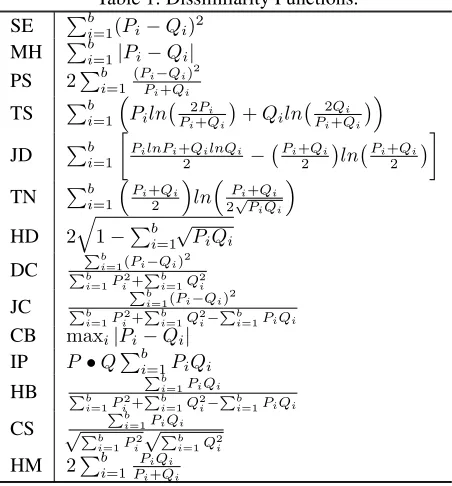
In this section, we list all compared functions, and point the interested reader to (Cha 2008) for a thorough survey on these measures. In our work, we have selected the following dissimilarity functions: Squared Euclidean (SE), Manhattan (MH), Probabilistic Symmetric (PS), Topsøe (TS), Jensen Difference (JD), Taneja (TN), Hellinger (HD), Dice (DC), Jaccard (JC), Chebyshev (CB), Inner Product (IP), Kumar-Hassebrook (HB), Cosine (CS), and Harmonic Mean (HM). All employed histogram distances, except for ORD, are de-scribed in Table 1, whereP andQare two normalized his-tograms of same lengthb.
Table 1: Dissimilarity Functions. SE Pb
i=1(Pi−Qi) 2
MH Pb
i=1|Pi−Qi| PS 2Pb
i=1
(Pi−Qi)2
Pi+Qi
TS Pb
i=1
Piln P2Pi
i+Qi
+Qiln P2Qi
i+Qi
JD Pb
i=1
PilnPi+QilnQi
2 −
Pi+Qi
2
ln Pi+Qi
2
TN Pb
i=1
P
i+Qi
2
ln Pi+Qi
2√PiQi
HD 2 q
1−Pb
i=1
√
PiQi
DC
Pb
i=1(Pi−Qi)2
Pb i=1Pi2+
Pb i=1Q2i
JC
Pb
i=1(Pi−Qi)2
Pb i=1Pi2+
Pb i=1Q2i−
Pb i=1PiQi
CB maxi|Pi−Qi| IP P•QPb
i=1PiQi
HB
Pb i=1PiQi
Pb i=1Pi2+
Pb i=1Q2i−
Pb i=1PiQi
CS
Pb i=1PiQi
√
Pb i=1Pi2
√
Pb i=1Q2i
HM 2Pb
i=1
PiQi
Pi+Qi
Although Cha (2008) surveys a larger set of distances, we decided to exclude from our analysis all monotonic trans-formations of these distances since they are deemed to pro-duce the same quantification estimates. This effect happens as, inDyS, we only search for the mixing parameter that pro-duces the lowest dissimilarity value and disregard the value itself. Monotonic transformations do not change the order of the values, and therefore we should find the same parame-ters. We also eliminated common but asymmetric functions so that we need not impose an arbitrary order between the mixed training distribution and the test distribution.
better understand such a distance, we note that in its original description, the histograms are normalized by multiplying every bin inP by|Q|and every bin inQby|P|. As such, each histogram is the allocation of |P| × |Q| units intob
bins. The objective of ORD is to find the least number of movements that need be done to transformQintoP, where one movement is the transference of a unit from a bin to aneighbor bin. There is always a possible transformation since both normalized histograms have the same number of units. This setting happens to be a univariate case of the min-imum difference of pair assignment(MDPA) of two distribu-tions, which is a special case of the Earth Mover’s Distance (EMD) (Rubner, Tomasi, and Guibas 1998). For this particu-lar case, the proposers of ORD introduce a greedy algorithm that can compute the distance in O(b), whereas the algo-rithms that are used to solve generic instances of EMD have higher time complexity. We note that the proposed algorithm also works when the histograms are normalized to have sum one, instead of|P| × |Q|. The Algorithm 1 describes the rationale of such distance.
Algorithm 1:Ordinal Distance
Data:Histograms to be comparedPandQ Result:Dissimilarity betweenPandQ 1 begin
2 diffsum←−0; 3 total cost←−0;
4 fori←1tolength(P)do
5 diffsum←−diffsum+ (P[i]−Q[i]); 6 total cost←−total cost+|diffsum|; 7 end
8 returntotal cost; 9 end
All histogram distances tested in our experiments, except for ORD, use each bin position in isolation. In other words, for each bin in one histogram, only one bin in the other his-togram can affect the distance. For this reason, we believe that ORD is less susceptible to the curse of dimensionality and bad parameterization of the number of bins, when it is greater than the ideal. For all other distances, as we increase the number of bins and consequently their granularity, non-zeroed bins are more likely to contain fewer observations and be countered by zeroed bins in the opposing histogram. In fact, when the number of bins is infinity, only observa-tions that are identical in both samples affect the distance and help decrease it. The distance is always one (the maxi-mum value) when there are no identical observations. ORD, on the other hand, is less affected by an increasing number of bins, since the difference between mismatching bins is accounted for and any pair of bins (and non-identical obser-vations) can affect the distance.
We introduce two dissimilarity functions that are suitable forDySand do not rely on histograms, as they are able to op-erate directly on the observations from training and test sam-ples. Such distances also carry the same benefits from the histograms approach, allowing for mixing pairs of
distribu-tions to be compared with a third distribution. However, they have the additional benefits of being immune to the curse of dimensionality while not losing information since they do not simplify the original data. We explain these distances in the following sections.
Mixable Kolmogorov Smirnov
The first distance is the Mixable Kolmogorov Smirnov (MKS) statistic. It is an adaptation of the Kolmogorov Smirnov (KS) (Kolmogorov 1933) statistic to compare two discrete empirical distributions and accounts for the first dis-tribution being a weighted mixture of two disdis-tributions.
Equation 3 formalizes such a dissimilarity, whereS+and
S−are the two samples that will be mixed together, accord-ing to the weights αand1−α, respectively, andZ is the third sample that represents the distribution to be compared with.
DM KS(S+, S−, α, Z) =
sup
x
|αFS+(x) + (1−α)FS−(x)−FZ(x)| (3)
whereFY(x)is the proportion of the observations inY that are lower or equal thanx.
SORD
The second dissimilarity function is the Sample ORD (SORD). SORD can be viewed as a special case of ORD where the number of bins is infinity: while ORD is the min-imum cost necessary to transform a histogram into another one, SORD is the minimum cost to transform a sample into another one.
If we are using SORD simply as a measurement of the difference between two samplesSandZ, every observation
xis weighted asw(x), defined as follows.
w(x) :=
|S|−1, x∈S
|Z|−1, x∈Z (4)
This way, both samples share the same total weight and the transformation is feasible. The cost of transforming a fraction fi,j,0 ≤ fi,j ≤ 1, of the i-th observation in S into thej-th observation inZ is c(i, j) = |fi,jw(Si)Si−
w(Zj)Zj|. The objective of SORD is therefore the follow-ing optimization problem.
minimize fi,j∀i,j
|S|
X
i
|Z|
X
j
c(i, j)
subject to
|Z|
X
j
fi,j= 1 ∀i
w(Zj)Zj =w(Si)Si
|S|
X
i
fi,j ∀j (5)
contains positive training observations and another with neg-ative training observations. This mixed sample is compared to a test sample. In this scenario, we have to adjust the weights of the observations in the mixed sample: positive observations share the same weight, proportional toα, and the negative ones share the same weight, inversely propor-tional toα.
SORD can be efficiently computed in O(|S ∪
Z|log|S∪Z|) with a greedy approach, where S and
Z are the two samples being compared. Algorithm 2 fully describes the distance computation with the necessary change to the weights whenSis a mixture (with parameter
α) of two samples (S+andS−).
Algorithm 2:SORD Dissimilarity Function
Data:Mixing samplesS+, S−, mixing factorα,
comparing sampleZ
Result:Dissimilarity betweenαS++ (1−α)S−andZ 1 begin
2 w0(x) :=
α|S+|−1, x∈S+
(1−α)|S−|−1, x∈S−
−|Z|−1, x∈Z
;
3 v←−sortedarray with∀x∈S+∪S−∪Z; 4 acc←−w0(v[1]);
5 total cost←−0;
6 fori←2tolength(v)do 7 δ←−v[i]−v[i−1];
8 total cost←−total cost+|δ×acc|; 9 acc←−acc+w0(v[i]);
10 end
11 returntotal cost; 12 end
Experimental Setup
In this paper, we make a comprehensible experimental eval-uation divided into two parts.
First, we hypothesize the existence of a relationship be-tween the size of the test sample and the number of his-togram bins that lead to the smallest error. The originalHDy
paper reports the estimated distribution based on the median across the use of varying number of bins from 10 to 110, with increments of 10. While this particular range may pro-vide good quantification errors when the test sample has a large number of observations, we want to verify if the more general DyS, which includes HDy, is significantly influ-enced by the number of bins, and how.
We note that until now, although the ideal number of bins has not been studied, a decision for this parameter may not be completely uninformed and can be based on important insights. Histograms with too many bins are negatively af-fected by two aspects. The first aspect is that if the sam-ple size is not large enough, large histograms can become too sparse, each bin can have excessively low weight, and ultimately, the dissimilarity function can face the curse of dimensionality. Exception for this rule is the use of ORD.
Notably, we note that ORD avoids being affected by such sparseness since the relation between neighbor dimensions is considered, rather than each dimension contributing in isolation to the magnitude of the distance. The second aspect is that a large number of bins has the implicit assumption of high precision for the scores. On the other hand, if there are too few bins, we may be unable to differentiate distributions. To verify the impact of the number of the bins, in all ex-periments, we vary the number of bins from 2 to 20 with increments of 2, and from 20 to 110 with increments of 10. The test sample size, on the other hand, varies from 10 to 100 with increments of 10 examples, and from 100 to 500 with increments of 100 examples.
Once we figure a satisfactory range for the number of bins for each dissimilarity function, we proceed to the second part of our evaluation. We consider a satisfactory range to be one that minimizes the largest number of bins necessary to obtain the smallest quantification errors for at least95%
of the cases. We analyze the impact of using different his-togram distances in theDySframework for binary quantifi-cation. With a fixed range of bins for each distance, we rank them according to the median quantification error produced by their use so that the top-ranked distances are those which lead to the smallest errors in each one of our experiments. We vary the test sample size from 10 to 500 in the afore-mentioned way. We analyze the behavior of the ranks for each dissimilarity function with a box plot.
For all experiments, we vary the positive class proportion from0%to100%with increments of1%, and for each pro-portion, we execute10runs with different test samples.
We performed preliminary experiments and concluded that Ternary Search (TSearch) suits all tested dissimilarity functions. For this reason, it is used for all of our experi-ments. We note that theαthat minimizes Squared Euclidean distance can be algebraically deduced inO(1). However, we also use TSearch for this distance to maintain experimental consistency across distances.
In the next section, we enumerate and describe the datasets used in our experiments.
Datasets
Each dataset was uniformly split into two halves: training and test. With the training half, we performed 10-fold cross-validation to obtain the training scores used byDyS. The full training half was also used to train a single scorer that was applied on the test half to get a test score set. Test samples were sampled from the test score set according to the set-tings described in the previous section regarding class pro-portion and size. One observation does not appear more than once in a single test sample, although it can appear in more than one test sample. This procedure was used to make the best use of our limited data.
We produced all scores using Random Forests with 200 trees. Also, we assess the performance of the quantifiers in our experiments using the Mean Absolute Error (MAE) (Se-bastiani 2018). MAE is the average of absolute differences between true (p) and predicted (pˆ) quantifications for a set of classesC, as shown in Equation 6.
M AE(p,pˆ) = 1
|C|
X
c∈C
|pˆ(c)−p(c)| (6)
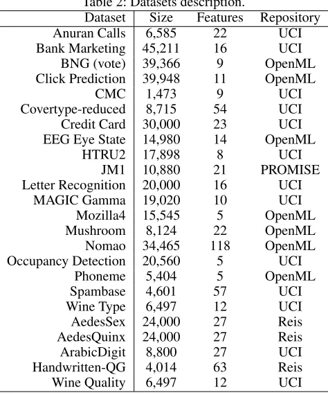
Table 2 presents a brief description of the datasets used in our experiments obtained from UCI (Dheeru and Karra Taniskidou 2017), OpenML (Vanschoren et al. 2013), PROMISE (Sayyad Shirabad and Menzies 2005), and Reis (dos Reis et al. 2018a) repositories. Specific citations are re-quested for Bank Marketing (Moro, Cortez, and Rita 2014), Credit Card (Yeh and Lien 2009), HTRU2 (Lyon et al. 2016), Mozilla4 (Koru, Zhang, and Liu 2007), Mushroom (Lincoff 1989), Nomao (Candillier and Lemaire 2012), and Occupancy Detection (Candanedo and Feldheim 2016). Ad-ditionally, we note that Jock A. Blackard and Colorado State University preserve copyright over Covertype.
Table 2: Datasets description.
Dataset Size Features Repository Anuran Calls 6,585 22 UCI Bank Marketing 45,211 16 UCI
BNG (vote) 39,366 9 OpenML Click Prediction 39,948 11 OpenML
CMC 1,473 9 UCI
Covertype-reduced 8,715 54 UCI Credit Card 30,000 23 UCI EEG Eye State 14,980 14 OpenML
HTRU2 17,898 8 UCI
JM1 10,880 21 PROMISE Letter Recognition 20,000 16 UCI
MAGIC Gamma 19,020 10 UCI Mozilla4 15,545 5 OpenML Mushroom 8,124 22 OpenML Nomao 34,465 118 OpenML Occupancy Detection 20,560 5 UCI
Phoneme 5,404 5 OpenML
Spambase 4,601 57 UCI
Wine Type 6,497 12 UCI AedesSex 24,000 27 Reis AedesQuinx 24,000 27 Reis ArabicDigit 8,800 27 UCI Handwritten-QG 4,014 63 Reis Wine Quality 6,497 12 UCI
Three observations about the datasets are due. First, Wine Type dataset is similar to Wine Quality. However, we want to differentiate between white and red wines, rather than the wine quality. Second, Covertype-reduced is a stratified sam-ple from Covertype due to its considerable size. The abbre-viated version is still large enough for our purposes. Ara-bicDigit is a preprocessed version of the original so that all examples have the same number of features (dos Reis et al.
2018a), and the objective is to predict the sex of the speaker rather than which digit is spoken. Finally, all the described datasets represent binary classification problems.
Experimental Evaluation
In this section, we present and discuss our experimental re-sults. One of our main questions regards a possible relation-ship between the number of bins and test sample size, to achieve the smallest quantification error. We are interested in knowing whether there is a test sample size for which it is better to use more or fewer bins than for another sam-ple size, for the same distance. In Figure 1, we illustrate the Mean Absolute Error (MAE) across datasets while varying the sample size, using the distance function Topsøe, as it represents the general behavior of other distances.
0.03 0.06 0.09
10 20 30 40 50 60 70 80 90
100 200 300 400 500 Test Sample Size
MAE
25 50 75 100 Bins
TS
Figure 1: Mean absolute quantification error averaged for all datasets, obtained withDySwith Topsøe and varying test sample size and number of histogram bins.
We can form three observations. First, the error is lower for more significant test samples, which is expected, since we are provided with more information about the test distri-bution. Second, for the Topsøe distance function, a smaller number of bins generally leads to smaller errors across all assessed test sample sizes. Third, greater sample sizes are less negatively impacted by a higher number of bins. This is explained by the lower sparseness of the bins with more observations in a higher dimensionality.
Both observations hold for all tested distances, except Co-sine, Harmonic Mean, Kumar-Hassebrook, Inner Product, and ORD. For the first four distances, errors are smaller for datasets with fewer observations, and a lower number of bins led to more significant errors. However, such distances per-formed very poorly: all of them led to errors greater than 70% on average, which is worse than a baseline that always predicts a positive class ratio of 50% and, consequently, ob-tains a maximum error of 50%. For this reason, Cosine, Har-monic Mean, Kumar-Hassebrook, and Inner Product will not be considered from now on.
sup-plemental material website1 contains figures for all other distances, which were omitted in this paper due to space constraints.
0.025 0.050 0.075 0.100
10 20 30 40 50 60 70 80 90
100 200 300 400 500 Test Sample Size
MAE
25 50 75 100 Bins
ORD
Figure 2: Mean absolute quantification error averaged for all datasets, obtained withDySwith ORD and varying test sample size and number of histogram bins.
In Figure 3, we observe that most of the best quantifica-tion results were obtained within up to 20 bins for all con-sidered distances, except for ORD. In Table 3, we detail this finding: we present the smallest upper limit for the number of bins that was necessary to constrain 90%, 95% and 100% of the smallest quantification errors obtained for each dis-tance. Hellinger Distance produced 95% of its best quantifi-cation results within the range from 2 to 14 bins. This find-ing contradicts the arbitrary range of 10 to 110 bins used by HDy’s original authors to calculate the median positive class ratio.
0 10 20 30 40 50 60 70 80 90 100 110
CB DC HD JC JD MH
ORD PS SE TN TS Dissimilarity Function
Number of bins
Frequency 50 100 150
Figure 3: Frequencies of the number of bins that produced the smallest quantification error for each distance function, inDyS.
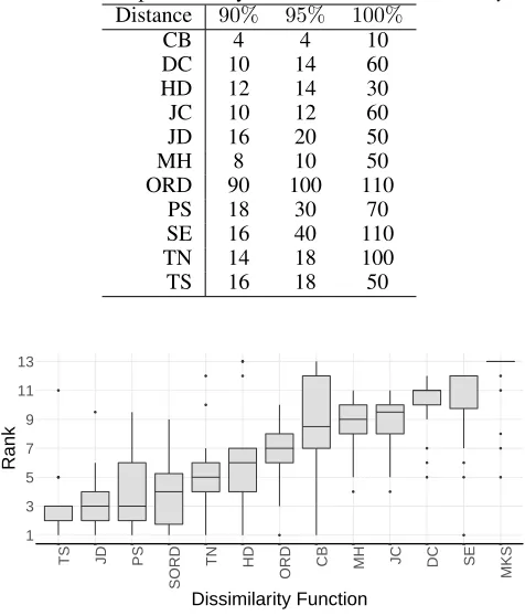
To rank the distances by quantification error, for each set-ting, we considered the median of the positive class ratio obtained withDyS while varying the number of bins. The number of bins ranges from 2 to the number of bins that are necessary to constrain 95% of the best results produced by the distance that was used, according to Table 3. The rank-ings are presented in Figure 4.
1
https://sites.google.com/site/andregustavom/research/dys
Table 3: Smallest upper bound for the number of histogram bins that encloses 90%, 95% and 100% of the smallest quan-tification errors produced by each distance function, inDyS.
Distance 90% 95% 100%
CB 4 4 10
DC 10 14 60
HD 12 14 30
JC 10 12 60
JD 16 20 50
MH 8 10 50
ORD 90 100 110
PS 18 30 70
SE 16 40 110
TN 14 18 100
TS 16 18 50
1 3 5 7 9 11 13
TS JD PS
SORD
TN HD
ORD CB MH
JC DC SE
MKS
Dissimilarity Function
Rank
Figure 4: Aggregation of several rank positions for differ-ent distances inDyS. Each quantification was predicted as a median of estimates obtained for different numbers of his-togram bins. The range of bins was individually tuned for each distance. Test sample size varied from 10 to 500.
We note that each distance had its range of bins tuned individually with the same datasets that were used for this comparison. Exceptions are SORD and MKS, which do not make use of this optimized parameter. This inserts bias into the comparison. On the other hand, if we had used the range from 10 to 110 bins, with increments of 10, as suggested by HDy’s authors, we would obtain the ranking presented in Figure 5. In this scenario, the top five best distances are the same. We note that ORD jumps to first place as it is less affected by large histograms, and Topsøe’s error increases.
1 3 5 7 9 11 13
SORD ORD
PS JD TS SE
MKS TN MH HD DC JC CB Dissimilarity Function
Rank
Figure 5: Aggregation of several rank positions for differ-ent distances inDyS. Each quantification was predicted as a median of estimates obtained for different numbers of his-togram bins. The range of bins was [10,110] for all dis-tances. Test sample size varied from 10 to 500.
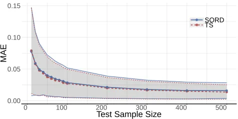
at tuning the number of bins to be used on the same datasets. Finally, we also potentially limited the best performance that SORD could achieve since we limited the size of the sam-ples, due to the algorithm’s higher computational cost in comparison with the histogram distances.
0.00 0.05 0.10 0.15
0 100 200 300 400 500
Test Sample Size
MAE
SORD TS
Figure 6: Comparison between SORD and Topsøe for vary-ing test sample size. The shaded area corresponds to the standard deviations from the measured points, and thinner curves set the limit of the shaded areas.
Additionally, ORD also performs closely to Topsøe, af-ter tuning, although not as close as SORD. This is true even though ORD fell from the second to the seventh rank posi-tion after the tuning process. However, this change of rank is due to an increase in the absolute performance of Topsøe, rather than a change in the performance of ORD. The latter is mostly unaffected by the rise in the number of bins (af-ter a minimum at which the different distributions become discernible).
Conclusions and Future Work
In this paper, we introducedDyS, a framework of Mixture Models for quantification. We analyzed the use of several histogram distances and concluded that Topsøe offers the smallest quantification errors across several datasets and test sample sizes when we tune the number of histogram bins.
0.00 0.05 0.10 0.15
0 100 200 300 400 500
Test Sample Size
MAE
ORD TS
Figure 7: Comparison between ORD and Topsøe for vary-ing test sample size. The shaded area corresponds to the standard deviations from the measured points, and thinner curves set the limit of the shaded areas.
We experimentally found that the best range for the number of bins inDySvaries for each distance function. While ORD is mostly unimpaired by an incorrect setting this parameter, for the majority of the distance functions, a suitable supe-rior limit was below20. Particularly, histograms with 14 or fewer bins provide at least 95% of the best quantification re-sults when using Hellinger Distance. This finding opposes the arbitrary range from 10 to 110 bins used by HDy’s orig-inal paper. Forig-inally, we introduced a new dissimilarity func-tion, SORD, that operates over observations rather than his-tograms, while still being compatible with the framework provided byDyS.
SORD outperforms all distances when they do not have their parameters tuned. On the other hand, when we tune the parameters, our parameter-free algorithm is outperformed by the Topsøe, Probabilistic Symmetric, and Jensen Dif-ference dissimilarity functions, respectively. However, even then, SORD presents better results than the HDy, the func-tion currently used by the state-of-art MMs, and is only slightly outperformed by Topsøe. ORD falls a little be-hind SORD, and even bebe-hind HDy. However, we argue that its performance is still competitive to Topsøe’s in practical terms and, as it is mostly unaffected by a wrong parame-terization of the number of bins. ORD is a viable and more time-efficient alternative to SORD when the tuning process cannot be done or is unreliable.
Acknowledgments
This study was financed in part by the Coordenac¸˜ao de Aperfeic¸oamento de Pessoal de N´ıvel Superior - Brasil (CAPES) - Finance Code PROEX-6909543/D, the Con-selho Nacional de Desenvolvimento Cient´ıfico e Tec-nol´ogico (CNPq, grant 306631/2016-4), the Fundac¸˜ao de Amparo a Pesquisa do Estado de S˜ao Paulo (FAPESP, grants 2016/04986-6, 2017/22896-7), and the United States Agency for International Development (USAID, grant AID-OAA-F-16-00072).
References
Bekker, J., and Davis, J. 2018. Estimating the class prior in positive and unlabeled data through decision tree induction. In Proceedings of the 32th AAAI Conference on Artificial Intelligence.
Candanedo, L. M., and Feldheim, V. 2016. Accurate occu-pancy detection of an office room from light, temperature, humidity and co2 measurements using statistical learning models.Energy and Buildings112:28–39.
Candillier, L., and Lemaire, V. 2012. Design and analy-sis of the nomao challenge active learning in the real-world. InProceedings of the ALRA: Active Learning in Real-world Applications, Workshop ECML-PKDD.
Cha, S.-H., and Srihari, S. N. 2002. On measuring the dis-tance between histograms.Pattern Recognition35(6):1355– 1370.
Cha, S.-H. 2008. Taxonomy of nominal type histogram distance measures.City1(2):1.
Dheeru, D., and Karra Taniskidou, E. 2017. UCI machine learning repository.
dos Reis, D.; Maletzke, A.; Silva, D. F.; and Batista, G. E. A. P. A. 2018a. Classifying and counting with recurrent contexts. InProceedings of the 24th ACM SIGKDD Interna-tional Conference on Knowledge Discovery and Data Min-ing, KDD ’18, 1983–1992. ACM.
dos Reis, D. M.; Maletzke, A. G.; Cherman, E.; and Batista, G. E. 2018b. One-class quantification. InProceedings of the European Conference on Machine Learning, 564–575. Esuli, A.; Sebastiani, F.; and Abbasi, A. 2010. Sentiment quantification.IEEE Intelligent Systems25(4):72–79. Forman, G. 2005. Counting positives accurately despite in-accurate classification. InEuropean Conference on Machine Learning, 564–575. Springer.
Forman, G. 2006. Quantifying trends accurately despite classifier error and class imbalance. InProceedings of the 12th ACM SIGKDD International Conference on Knowl-edge Discovery and Data Mining, KDD ’06, 157–166. ACM.
Forman, G. 2008. Quantifying counts and costs via classifi-cation. Data Mining and Knowledge Discovery17(2):164– 206.
Gao, W., and Sebastiani, F. 2016. From classification to quantification in tweet sentiment analysis. Social Network Analysis and Mining6(1).
Gonz´alez, P.; Casta˜no, A.; Chawla, N. V.; and Coz, J. J. D. 2017a. A review on quantification learning. ACM Comput-ing Surveys (CSUR)50(5):74.
Gonz´alez, P.; D´ıez, J.; Chawla, N.; and del Coz, J. J. 2017b. Why is quantification an interesting learning prob-lem? Progress in Artificial Intelligence6(1):53–58.
Gonz´alez-Castro, V.; Alaiz-Rodr´ıguez, R.; and Alegre, E. 2013. Class distribution estimation based on the hellinger distance.Information Sciences218:146 – 164.
Kolmogorov, A. 1933. Sulla determinazione empirica di una lgge di distribuzione. Inst. Ital. Attuari, Giorn.4:83–91. Koru, A. G.; Zhang, D.; and Liu, H. 2007. Modeling the effect of size on defect proneness for open-source soft-ware. InPredictor Models in Software Engineering, 2007. PROMISE’07: ICSE Workshops 2007. International Work-shop on, 10–10. IEEE.
Lincoff, G. H. 1989. The audubon society field guide to North American mushrooms. Technical Report No. 635.8 L5.
Lyon, R. J.; Stappers, B.; Cooper, S.; Brooke, J.; and Knowles, J. 2016. Fifty years of pulsar candidate selection: from simple filters to a new principled real-time classifica-tion approach. Monthly Notices of the Royal Astronomical Society459(1):1104–1123.
Maletzke, A.; dos Reis, D.; Cherman, E.; and Batista, G. 2018. On the need of class ratio insensitive drift tests for data streams. In Proceedings of the Second International Workshop on Learning with Imbalanced Domains: Theory and Applications, volume 94 of Proceedings of Machine Learning Research, 110–124. ECML-PKDD, Dublin, Ire-land: PMLR.
Moro, S.; Cortez, P.; and Rita, P. 2014. A data-driven ap-proach to predict the success of bank telemarketing. Deci-sion Support Systems62:22–31.
P´erez-G´allego, P.; Casta˜no, A.; Quevedo, J. R.; and del Coz, J. J. 2019. Dynamic ensemble selection for quantification tasks.Information Fusion45:1–15.
Pollard, D. 2002. A user’s guide to measure theoretic prob-ability, volume 8. Cambridge University Press.
Rubner, Y.; Tomasi, C.; and Guibas, L. J. 1998. A metric for distributions with applications to image databases. In
Computer Vision, 1998. Sixth International Conference on, 59–66. IEEE.
Sayyad Shirabad, J., and Menzies, T. 2005. The PROMISE repository of software engineering databases. School of In-formation Technology and Engineering, University of Ot-tawa, Canada.
Sebastiani, F. 2018. Evaluation measures for quantification: An axiomatic approach. arXiv preprint arXiv:1809.01991. Vanschoren, J.; van Rijn, J. N.; Bischl, B.; and Torgo, L. 2013. Openml: Networked science in machine learning.