Layer-Wise Learning Strategy for Nonparametric Tensor Product Smoothing Spline Regression and Graphical Models

Layer-Wise Learning Strategy for Nonparametric Tensor

Product Smoothing Spline Regression and Graphical Models

Kean Ming Tan [email protected]

Department of Statistics University of Michigan Ann Arbor MI, 48109

Junwei Lu [email protected]

Department of Biostatistics

Harvard T.H. Chan School of Public Health Boston MA, 02115

Tong Zhang [email protected]

Department of Computer Science and Engineering Department of Mathematics

The Hong Kong University of Science and Technology Clear Water Bay, Hong Kong.

Han Liu [email protected]

Department of Electrical Engineering and Computer Science Northwestern University

Evanston IL, 60208

Editor:Sara van de Geer

Abstract

Nonparametric estimation of multivariate functions is an important problem in statisti-cal machine learning with many applications, ranging from nonparametric regression to nonparametric graphical models. Several authors have proposed to estimate multivariate functions under the smoothing spline analysis of variance (SSANOVA) framework, which assumes that the multivariate function can be decomposed into the summation of main effects, two-way interaction effects, and higher order interaction effects. However, existing methods are not scalable to the dimension of the random variables and the order of inter-actions. We propose a LAyer-wiSE leaRning strategy (LASER) to estimate multivariate functions under the SSANOVA framework. The main idea is to approximate the multivari-ate function sequentially starting from a model with only the main effects. Conditioned on the support of the estimated main effects, we estimate the two-way interaction effects only when the corresponding main effects are estimated to be non-zero. This process is con-tinued until no more higher order interaction effects are identified. The proposed strategy provides a data-driven approach for estimating multivariate functions under the SSANOVA framework. Our proposal yields a sequence of estimators. To study the theoretical prop-erties of the sequence of estimators, we establish the notion of post-selection persistency. Extensive numerical studies are performed to evaluate the performance of LASER.

Keywords: Persistency, nonparametric regression, nonparametric graphical models, se-quential algorithm, model selection

c

1. Introduction

Much progress has been made in nonparametric estimation of univariate functions. However, nonparametric estimation of multivariate functions remains a challenging problem due to the curse of dimensionality. A number of algorithms were proposed to estimate low-dimensional multivariate functions, but there are few practical algorithms for estimating multivariate functions with higher dimension.

To address this issue, many authors proposed to restrict the multivariate function to some specific model classes. One popular model class is the additive model in which the high-dimensional multivariate functionf(·) is decomposed into the sum ofdone-dimensional functions (Stone, 1985; Hastie and Tibshirani, 1990). To increase the flexibility of the ad-ditive model to accommodate situation in which interactions among the variables may be present, Lin (2000) proposed to estimate the multivariate function under the smoothing spline analysis of variance (SSANOVA) framework. More specifically, Lin (2000) proposed to decompose the d-dimensional function f(·) as the summation of some constantµ, one-dimensional functions (main effects), two-one-dimensional functions (two-way interaction ef-fects), and so on:

f(x) =µ+

d

X

j=1

fj(xj) +

X

j<k

fjk(xj, xk) +· · · . (1)

We refer the reader to Lin (2000) and Gu (2013) for a detailed discussion of such models. Most existing methods under the SSANOVA framework truncate (1) to the rth order interaction effects. Even so, existing methods are computationally intensive and are not scalable to the dimension of the random variables d and the order of the interaction term

r. For instance, to fit a nonparametric regression model under the SSANOVA framework with the rth order interaction, it involves simultaneously fitting O(dr) terms and is often infeasible when both d and r are large (Lin and Zhang, 2006). Thus, one way to reduce the computation complexity is to consider only the two-way interaction terms and remove all of the higher order interaction terms from the model (Lin, 2000; Zhang et al., 2004; Lin and Zhang, 2006; Jeon and Lin, 2006; Yau et al., 2012).

involves modeling d₂

terms. We refer the reader to Haris et al. (2016) for a comprehensive review of the literature.

In this paper, we propose a framework to estimate multivariate functions that take the form (1) without restricting it to only modeling the two-way interaction terms. We impose a hierarchical structure on the higher order interaction terms under the SSANOVA framework. Let J, J0 ⊆ {1, . . . , d}. Given a d-dimensional function f, we denote fJ as

the |J|th order interaction term in f with variables {xj}j∈J. We impose the hierarchical

structural assumption that

fJ = 0 =⇒ fJ0 = 0, if J ⊂J0. (2)

In other words, we assume that a higher order interaction is not active when some of the lower order terms containing some variables that belong to the higher order term are not active. For instance, if the main effect of thejth variablefj = 0, then any higher order term

that involves thejth variable is not active. The hierarchical structural assumption is plau-sible in many data applications. For instance, in the context of nonparametric regression, the hierarchical structural assumption implies that the main effects are more important in modeling the response than the higher order interactions. Therefore, if the leading order in-teraction function does not have any explanatory power, the higher order inin-teraction terms should be inactive. The hierarchical assumption in (2) can be thought of as an extension of the strong heredity assumption to modeling higher order interaction terms.

Under the hierarchical structural assumption, we propose a layer-wise learning algo-rithm to estimate multivariate functions under the SSANOVA framework. Our algoalgo-rithm sequentially estimates the multivariate function starting from the main effects to the higher order interaction terms. In each step of our algorithm, we utilize the support of the esti-mated function from the previous step and estimate the function based on the hierarchical structural assumption in (2). This process is continued until no more higher order interac-tion effects are active. Instead of fitting the SSANOVA model withd+ d₂

+· · ·+ d_r terms, our proposal fits the SSANOVA model with at most d+ s1

2

+· · ·+ sr−1

r

terms, wheresk

is the cardinality of the support of the estimatedkth order interaction effects. Thus, our al-gorithm is scalable to modeling higher order interaction terms with large dimensiond. Our proposed framework can be interpreted as an extension of Hao and Zhang (2014) and Hao et al. (2018) to modeling multivariate functions, as well as modeling higher order interac-tion effects. Compared to Radchenko and James (2010) that involves modeling all two-way interaction terms, our approach is a multi-stage procedure and therefore is computationally efficient and scalable for problems with large dimensiond.

To quantify the theoretical properties of our estimator, we propose the notion of post-selection persistency. We show that conditioned on the support of the estimator obtained from the (r−1)th step of the algorithm, the excessive risk between the estimator obtained from therth step and the best rth order SSANOVA model converges to zero. Our results hold without assuming that the true multivariate function takes the form of the SSANOVA model in (1). In addition, we impose minimal distributional assumptions on the data.

func-tional component in the SSANOVA decomposition in (1). We then propose the layer-wise learning algorithm for estimating multivariate function under a generic loss function. We apply the proposed algorithm to fitting nonparametric regression and graphical models in Sections 3 and 4, respectively. Numerical studies are performed in Section 5. We close with a discussion in Section 6. The proofs of the theoretical results are given in the Appendix.

2. Layer-Wise Learning Strategy

We describe the problem setup and define some notation. We then propose the layer-wise learning strategy for estimating nonparametric functions with high order interactions.

2.1 Problem Setup and Notation

We start with a brief overview of the tensor product space of Sobolev spaces and refer the reader to Lin (2000) for a detailed review. For any non-negative integerm, themth order Sobolev space with a univariate variable xj ∈[0,1] is defined as

H_jm=

g g

(ν)_{is absolutely continuous for 0≤ν ≤m−1; g}(m)_∈L2_([0,1]); Z 1

0

g(u)du= 0

,

whereg(ν)is theνth order derivative ofg. The Sobolev norm for functiong∈H_jm is defined as

kgk2 Hm

j =

m

X

ν=0

Z 1

0

h

g(ν)(u)i2du.

For notational convenience, let [d] = {1, . . . , d}. Let J ⊆ [d] be an index set with cardinality |J|=r, and let HJ =⊗j∈JHjm be the completed tensor product space of Hjm

for all j ∈J. We assume that gJ ∈ HJ. Letα= (α1, . . . , αr)T be an r-dimensional vector

with integer entries and letkαk1 =Pr_i=1αi ≤m. Let J ={j1, . . . , jr}. The Sobolev norm

for the multivariate functiongJ ∈ HJ is defined as

kgJk2HJ =

X

α:kαk1≤m

kDαgJk2 where Dα=

∂kαk1

∂xα1

j1 · · ·∂x

αr

jr

. (3)

We define the smoothing spline ANOVA function class as

{1} ⊕ d

X

j=1

H_jm ⊕ X J⊆[d],|J|=2

H_J ⊕ X

J⊆[d],|J|=3

H_J ⊕ · · · .

Each functional component in the SSANOVA decomposition (1) lies in a subspace in the orthogonal decomposition of the tensor product space. We define therth order smoothing spline ANOVA function class as

H(r)={1} ⊕ d

X

j=1

H_jm ⊕ X J⊆[d],|J|=2

H_J ⊕ · · · ⊕ X

J⊆[d],|J|=r

H_J. (4)

2.2 Layer-Wise Learning Algorithm

We propose the layer-wise learning algorithm to learn ad-dimensional multivariate function under the SSANOVA framework. Recall from (2) that we assume a hierarchical structure on the model, i.e., higher order interaction terms are not active when the lower order terms are not active. To this end, we define some additional notation that will be used throughout the paper. Given a set S ⊆ {J | J ⊆ [d]}, let |S|max = max{|I| | I ∈ S} be the largest

cardinality among the sets in S. In addition, we define

σ(S) =  



I

|I|=|S|max+ 1, I ⊆

[

|J|=|S|max, J∈S

J

 



.

For example, if S = {{1},{2},{3}}, then σ(S) = {{1,2},{1,3},{2,3}}. For notational convenience, we also define δ(S) =S ∪σ(S) throughout the paper. Thus, in this example,

δ(S) ={{1},{2},{3},{1,2},{1,3},{2,3}}.

The main crux of our proposal is to estimate the multivariate function sequentially starting from the main effects. Using the support of the estimated function from the previous step, we estimate the multivariate function by considering higher order terms only when the lower order terms are estimated to be non-zeros. Let D be the data and letLn(D, f)

be a generic loss function for estimatingf. At the first step of the algorithm, we estimate the function f subject to f ∈ H(1)_{. In other words, f is assumed to be additive and we}

propose to estimatef by

b

f(1)= argmin

f∈H(1)

L_n(D, f), subject to

d

X

j=1

kPj(f)k2≤τ, (5)

wherePj(f) is the orthogonal projection off ontoHjm. The penalty term

Pd

j=1kPj(f)k2≤ τ can be interpreted as an`1constraint across components to encourage sparsity, and an`2

constraint within components to encourage smoothness. The tuning parameter τ controls the number of main effects that are estimated to be non-zero.

Let S(1) _{be the support of}

b

f(1), that is, S(1) _{= {j | P}

j(fb(1)) 6= 0}. Given the support S(1)_{, we fit the following model at the second step of our algorithm}

b

f(2)= argmin

f∈H(2)_,S(f)=δ(S(1)₎

Ln(D, f),

subject to X

j∈S(1)

kPj(f)k22+

X

{j1,j2}∈σ(S(1))

kPj1j2(f)k2 ≤τ,

(6)

wherePj1j2(f) is the orthogonal projection off ontoH

m j1⊗H

m

j2. For notational convenience,

letS(f) be the support off. At the second step of our algorithm, we update both the main effects and the second order interactions, with the support of the function constrained on

S(f) = δ(S(1)_{). Since we have selected the support for the main effects, we use a ridge}

penalty to encourage smoothness for the main effects.

More generally, letS(r−1) _{be the support identified at the (r−1)th step of our proposed}

Algorithm 1 Layer-Wise Learning Method (LASER). Input: : DataD.

Initialize: S(0)_=∅,σ(S(0)_{) ={1, . . . , d}, and r= 1.}

repeat

1. Update the function withrth order interaction effects:

b

f(r)= argmin

f∈H(r)_,S(f)=δ(S(r−1)₎

Ln(D, f),

subject to X

J∈S(r−1)

kPJ(f)k22+

X

J∈σ(S(r−1)₎

kPJ(f)k2 ≤τ.

2. Update the support S(r)_=S(

b

f(r)). 3. r←r+ 1.

until S(r−1) _=S(r)_.

Output: A sequence of estimators{fb(`)}r<sub>`=1</sub>.

the |J|th order interaction effect space ⊗_j∈JHjm. At the rth step of the algorithm, we fit

the model

b

f(r)= argmin

f∈H(r)_,S(f)=δ(S(r−1)₎

L_n(D, f),

subject to X

J∈S(r−1)

kPJ(f)k22+

X

J∈σ(S(r−1)₎

kPJ(f)k2≤τ.

(7)

We continue this process until no more higher order interaction effects are estimated to be non-zero. We summarize the proposed method in Algorithm 1. Step 1 in Algorithm 1 depends on a specific loss function Ln(D, f). We will present the details for Step 1 in

the context of nonparametric regression and nonparametric graphical models in Sections 3 and 4, respectively.

2.3 Post-Selection Persistency

We first provide a brief review of the definition of persistency introduced by Greenshtein and Ritov (2004). We define the risk of some function f as R(f) =E[Ln(D, f)]. An estimator

b

f is said to be persistent relative to a class of functionF if

R(fb)− inf

f∈FR(f) =oP(1). (8)

In other words, the risk of the estimatorfbis consistent to that of the oracle function under the model classF. In the statistical literature, many authors have shown that the estimators for various statistical models are persistent (see, for instance, Greenshtein and Ritov, 2004 for the lasso regression, and Ravikumar et al., 2009 for the sparse additive model). However, most of the existing results on persistency are derived for a single estimator, and not much work has been done to characterize a sequence of estimators.

yields a sequence of estimators {fb(`)}r<sub>`=1</sub>. Also recall that we denoteS(r−1) to be the sup-port of fb(r−1). Let F(r) be some function class with support constrained on δ(S(r−1)) = S(r−1) _∪σ(S(r−1)_{). Conditioned on the support S}(r−1)_{, we say that}

b

f(r) is post-selection persistent if

R(fb(r))− inf

f∈F(r)R(f) =oP(1). (9)

We will show that our proposed estimators are post-selection persistent in the context of nonparametric regression and nonparametric graphical models in Sections 3 and 4, respec-tively.

3. Nonparametric Regression

We apply the layer-wise learning strategy to the setting of nonparametric regression. We consider a nonparametric regression problem of a univariate response Y ∈ R on a d -dimensional covariates X ∈[0,1]d:

Y =f(x) +,

where is the random noise variable. It is generally agreed upon in the literature that estimating a general multivariate function without restricting the function into a smaller function classF is infeasible.

Hastie and Tibshirani (1990) and Stone (1985) introduced a class of additive models of the form f(x) =Pd

j=1fj(xj), which decomposed the multivariate functionf(·) into the

summation of d univariate functions. One caveat of the additive model is the assumption that there are no interaction terms among the covariates. To address this issue, Lin (2000) proposed to estimate f(·) by assuming that it takes the form in (1) in the nonparametric regression setting. However, their proposal is infeasible for high-dimensional problem in which the number of covariates dand the order of interaction terms are large. Thus, they truncated (1) to only modeling two-way interaction terms. More specifically, they considered the following decomposition forf(·):

f(x) =µ+

d

X

j=1

fj(xj) +

X

j<k

fjk(xj, xk).

Several authors have extended the aforementioned models to perform variable selection and estimation simultaneously (among others, Lin and Zhang, 2006; Ravikumar et al., 2009). However, Ravikumar et al. (2009) models only the main effects and Lin and Zhang (2006) is computationally infeasible for large d problems even when they model only the second order interaction terms. The nonparametric regression literature is vast and we refer the reader to several recent proposals for more references (see, Tibshirani, 2014; Fan et al., 2015; Lou et al., 2016).

3.1 Method and Optimization Problem

Let (y1,x1), . . . ,(yn,xn) be n independent pairs of observations. We assume that the

co-variates x1, . . . ,xn are standardized such that xi ∈ [0,1]d and that yi = f(xi) +i with

E[i] = 0 and E[i2]<∞. The functionf(·) is an arbitrary function and is not assumed to

take the form of (1). To approximate the function f(·), we fit the model in (7) with the squared error loss function L_n(D, f) =Pn

i=1(yi−f(xi))2/n. This yields the optimization

problem

minimize

f∈H(r)_,S(f)=δ(S(r−1)₎

1

n n

X

i=1

(yi−f(xi))2,

subject to X

J∈S(r−1)

kPJ(f)k22+

X

J∈σ(S(r−1)₎

kPJ(f)k2≤τ,

(10)

whereτ >0 is a positive tuning parameter.

It is useful to write the functionf(·) in terms of its basis function. Let{φj`, `= 1,2, . . .}

denote a uniformly bounded basis with respect to H_jm. Given J = {j1, . . . , jr}, for any fJ ∈ HJ, the basis expansion offJ is

fJ =

X

1≤k1,...,kr<∞

θk1···kr

j1···jr φj1k1(xj1)· · ·φjrkr(xjr). (11)

In practice, we approximate (11) by its kth order basis expansion

e

fJ =

X

1≤k1,...,kr≤k

θk1···kr

j1···jr φj1k1(xj1)· · ·φjrkr(xjr) =φ

T

J(x)θJ, (12)

whereθJ = vec({θjk11···jkrr}) andφJ(x) = vec({φj1k1(xj1)· · ·φjrkr(xjr)}).

LetΦJ denote then×k|J|matrix with rowsφJ(x1), . . . ,φJ(xn) and lety= (y1, . . . , yn)T.

We approximate (10) in terms of the kth order basis expansion:

minimize θJ,S(f)=δ(S(r−1))

1

n

y−

X

J∈S(f)

ΦJθJ

2 2,

subject to 1

n

X

J∈S(r−1)

kΦJθJk22+

1

√

n

X

J∈σ(S(r−1)₎

kΦJθJk2 ≤τ.

(13)

Instead of solving optimization problem in (13) directly, we consider solving the following problem

minimize θJ,S(f)=δ(S(r−1))

1

n

y−

X

J∈S(f)

ΦJθJ

2 2+λ

1

n

X

J∈S(r−1)

kΦJθJk22+

1

√

n

X

J∈σ(S(r−1)₎

kΦJθJk2

(14)

Algorithm 2 Block Coordinate Descent Algorithm for Solving (14).

Initialize θb

(0) J .

repeat

forJ ∈δ(S(r−1)_{) do}

Update the coefficients:

b

θ_J(t)= ΦT_JΦJ

−1

ΦT_Jy−ΦT_J X

J0_∈{δ(S(r−1)_)\J}

ΦT_J0θb

(t−1) J0

.

Penalize the coefficients:

b

θ(t)_J =   

  b

θ_J(t)/(1 +λ) if J ∈ S(r−1)_,

1−

√ nλ 2kΦJθb

(t) J k2

+

b

θ_J(t) if J ∈σ(S(r−1)_),

where (a)+= max(0, a).

end for

Updatet=t+ 1.

until converge such thatP

J

θb

(t) J −θb

(t−1) J

2 ≤.

It can be verified that when r = 1, (14) is equivalent to the sparse additive model in Ravikumar et al. (2009).

Since (14) is quadratic in terms of θJ and both the penalty terms are convex, standard convexity theory implies the existence of a global minimizer. We propose a block coordinate descent algorithm to solve (14), which details are given in Algorithm 2. The convergence of block coordinate descent algorithm is studied in Tseng (2001). The derivation of Algo-rithm 2 is straightforward and hence omitted. In this section, our estimation procedure and algorithm are designed based on basis representation of the functions. We note that in principle, other nonparametric methods such as that of Wang et al. (2016) and Benkeser and van der Laan (2016) can be used to estimate the individual functions in our framework.

3.2 Post-Selection Persistency for Nonparametric Regression

In this section, we show that the sequence of estimators obtained from our proposal is post-selection persistent. The population version of the optimization problem in (10) is

minimize

f∈H(r)_,S(f)=δ(S(r−1)₎E

(Y −f(X))2,

subject to X

J∈S(r−1)

E(PJ(f))2

+ X

J∈σ(S(r−1)₎

p

E[(PJ(f))2]≤τ, E[PJ(f)] = 0,

(15)

minimize

g∈H(r)_,β

J,S(g)=δ(S(r−1)) E



 

Y −

X

J∈δ(S(r−1)₎

βJgJ(XJ)





2 ,

subject to X

J∈S(r−1)

β_J2+ X

J∈σ(S(r−1)₎

|βJ| ≤τ, E[PJ(g)] = 0, E(PJ(g))2

= 1.

(16)

Problems (16) and (15) are equivalent in the sense that their solutions are equivalent. A similar formulation was also considered in Ravikumar et al. (2009) for sparse additive models.

Let (X, Y) denote a new pair of independent data and define the predictive risk as

R(f) =E(Y −f(X))2.

In this section, we assume that our estimatorfb(r)is chosen to minimize the empirical version of (16). Let

F(r)₌

  

f :f(x) = X

J∈δ(S(r−1)₎

βJgJ(xJ),E[gJ] = 0,kgJkHJ ≤1,

X

J∈S(r−1)

β_J2+ X

J∈σ(S(r−1)₎

|βJ| ≤τ

  

.

The following theorem establishes that the sequence of estimators is post-selection persis-tent.

Theorem 1. Let s0 = 1and let sr−1 be the cardinality of the supportS(r−1). Conditioned onS(r−1)_{, under the square error risk R(f) =}

E[(Y −f(X))2]and for any 1≤r <2m, we

have

R(fb(r))− inf

f∈F(r) R(f) =OP



τ2· s

rs2

r−1logd n



.

Thus, if τ =o([n/(rs2_r−1logd)]1/4), the estimator fb(r) is post-selection persistent.

In other words, Theorem 1 states that conditioned on the selected support on the (r−

1)th step of our proposed method, S(r−1)_{, the estimator}

b

f(r) converges to the best rth order approximation of the form (1) with support constrained on δ(S(r−1)_{). Given the}

supportS(r−1)_{, the terms}

r−1 is a fixed constant that is much smaller thann. The proof of

Theorem 1 involves obtaining the bracketing number of some function classes and applying empirical process tools to obtain an upper bound of the supremum between the empirical and the expected value of the function. The conditionr < 2m in Theorem 1 is needed to guarantee that the integral of the log bracketing number is well defined. The details are given in Appendix A.

3.3 From Post-Selection Persistency to Persistency

Post-selection persistency results can serve as motivations for intermediate steps of LASER. However, the results do not concern properties of the final estimator. In this section, we establish sufficient conditions such that a post-selection persistency result can be strengthen into a persistency result for the final estimator. For simplicity, we consider nonparametric regression models with two-way interaction terms, i.e., f ∈ H(2)_.

In general, without any conditions on the bivariate functions fjk, it is extremely

chal-lenging to show that the main effects fj can be identified without modeling the two-way

interaction effects. This problem is related to proving model selection consistency under model misspecification for sparse additive model, and such theoretical results have not been well established in the literature. In fact, the same problem is not well understood in the context of linear regression with two-way interaction effects until recently (Hao et al., 2018). In the following, we impose sufficient conditions on the bivariate functions such that the active main effects can be identified at the first stage of LASER in the context of nonparametric regression. Therefore, conditioned on the correctly identified main effects, the estimator obtained from the second stage is persistent. With some abuse of notation, let ¯S(1) _{and ¯S}(2) _{be two sets containing indices for the underlying active main and bivariate}

effects, respectively. Assume that ¯S(2)_{satisfies the hierarchical structural assumption in (2).}

Recall from Section 3.1 that we approximate the main effects by its kth order basis expansion, i.e.,θ∗= argmin_θ=(θT

1,...,θTd)Tk

Pd

j=1fj−Pdj=1θTjφjk22. In the following

propo-sition, our conditions are written in terms of an approximation of both the main and the partial derivatives of the bivariate function using first order basis expansion. To this end, we define some additional notation. Given a bivariate functiong(x1, x2), let

g(2)(x1, x2)

a1,a2 =g(a1, a2) +

X

j∈{1,2}

∂g(a1, a2) ∂xj

(xj −aj) +

1 2

∂2g(a1, a2)

∂x2_j (xj−aj) 2

,

and

β∗= argmin β=(βT

1,...,βTd)T

d

X

j=1 fj +

X

s<t f_st(2)

1/2,1/2− d

X

j=1 β_jTφj

2 2 .

The following proposition establishes that the true underlying support, ¯S(1)_{, is a subset of}

the estimated support from first stage of LASER,S(1)_.

Proposition 1. Assume that f ∈ H(2)_{. Suppose that there exist a positive constant C} min such that the minimum eigenvalueλmin(ΦTS¯(1)ΦS¯(1))≥C_min>0. Letρ∗_n= min_j∈S¯(1)kβ∗_jk∞ and q_n∗ = kP

(s,t)∈S¯(2)∂_x2_sxtfstk∞. Assume that

p

|S¯(1)_|k·q∗

n/ρ∗n = o(1), √

kq_n∗/λ = o(1), and

1

ρ∗_n

q

log(|S¯(1)_|k)/n+|S¯(1)_|3/2_/k+λq_|S¯(1)_|k

=o(1).

We haveP(S(1)⊇S¯(1))→1.

pointed out, this implies that the bivariate functions should be close to linear, relative to the main effects. We have removed the incoherence condition in Ravikumar et al. (2009) and we now allow the active and non-active main effects to be correlated. Relaxing the imposed assumptions on the bivariate functions is out of the scope of this paper, and we leave it as an open problem for future research.

4. Nonparametric Graphical Models

Undirected graphical models, also known as Markov random field, have been used exten-sively to model the conditional dependence relationships among a set of random variables. In a graph, each node represents a random variable and an edge between two nodes indicates that the two random variables are conditionally dependent, given all of the other variables. LetX be ad-dimensional random variable with joint density function of the form

p(x) = 1

Z(f)exp(−f(x)), (17)

whereZ(f) =R

exp(−f(x))dxis the partition function such that the densityp(x) integrates to one. By the Hammersley-Clifford theorem, a set of random variablesX forms a Markov random field with respect to a graph G if f(x) takes the form f(x) = P

J∈JGfJ(xJ),

where JG is a set of all cliques in G and fJ is the potential function. For a set J ⊆ [d],

if fJ(xJ) 6= 0, then the set of random variables XJ forms a clique and are conditionally

dependent given all of the other variables.

Currently, most of the research on graphical models are limited to the case when the maximal clique is of size two. This is referred to as the pairwise Markov random field with the following joint density

p(x) = 1

Z(f)exp  

 −

d

X

j=1

fj(xj)−

X

j<k

fjk(xj, xk)

 



. (18)

Under the pairwise Markov random field, thejth andkth random variables are conditionally independent if and only if fjk(xj, xk) = 0. The pairwise Markov random field in (18) is

fully nonparametric and consists of many recently studied pairwise graphical models as its special cases.

Example 1. Gaussian graphical models: Let X ∼ Nd(0,Σ) and let Θ = Σ−1 be the inverse covariance matrix. The Gaussian graphical model has joint density

p(x)∝exp  

 −1

2

d

X

j=1

Θjjx2j− d−1

X

j=1

X

k>j

Θjkxjxk

 



.

Example 2. Exponential family graphical models: The exponential family graphical model has joint density

p(x)∝exp  



d

X

j=1

(t(xj) +C(xj)) + d−1

X

j=1

X

k>j

Θjkt(xj)t(xk)

 



,

where t(xj) is a univariate sufficient statistics function, C(xj) is some function ofxj spec-ified by the exponential family distribution, and Θjk is the canonical parameter. Thus, this is a special case of (18) with fjk(xj, xk) = −Θjkt(xj)t(xk) and fj(xj) = −t(xj)−C(xj). This model is recently studied by many authors (see, for instance, Yang et al., 2013, 2015; Tan et al., 2016; Yang et al., 2018; Chen et al., 2014)

Example 3. Nonparanormal graphical models: Let g={g1, . . . , gd} be a set of monotone univariate functions. A d-dimensional random vector X has a nonparanormal distribution X ∼NPNd(g,Σ) if g(X)∼Nd(0,Σ). Let Θ=Σ−1. Then, the nonparanormal graphical model has joint density

p(x)∝exp  



d

X

j=1

−1

2Θjjgj(xj)

2_{+ log} g0_j(x_j)

− d−1

X

j=1

X

k>j

Θjkgj(xj)gk(xk)

 



.

This is a special case of (18) withfjk(xj, xk) = Θjkgj(xj)gk(xk)andfj(xj) = Θjjgj(xj)2/2−

log|g_j0(xj)|. This model is studied in Liu et al. (2009) and Liu et al. (2012).

We consider modeling the Markov random field in (17) under the SSANOVA framework, that is, the function f(·) can be decomposed as in (1). This general model has been considered in the literature and an estimate off(·) can be obtained by optimizing over the penalized maximum likelihood function (see, for instance, Leonard, 1978; Silverman, 1982; Gu and Wang, 2003; Jeon and Lin, 2006). However, due to the log-partition functionZ(f), the proposed algorithms are not scalable to large dimension and higher order interaction terms. To the best of our knowledge, most methods involve truncating the functional decomposition (1) to only modeling the two-way interaction terms, which corresponds to pairwise nonparametric graphical models in (18).

In this section, we propose a novel method to estimate nonparametric graphical models of the form (17) without restricting it to only modeling two-way interaction terms. More specifically, we are interested in estimating nonparametric graphical models with joint den-sity function

p(x) = 1

Z(f)exp(−f(x)) and f(x) =µ+

d

X

j=1

fj(xj) +

X

j<k

fjk(xj, xk) +· · · .

4.1 Score Matching Loss

The score matching loss function was introduced to estimate densities of the form (17), which involves a computationally intractable log-partition functionZ(f). In the following, we provide a brief discussion on the score matching loss and refer the reader to Hyv¨arinen (2005) and Hyv¨arinen (2007) for more details. LetX be ad-dimensional continuous random vector with distributionP and joint density functionp(·). For a twice differentiable function

f :Rd→R, we define the Laplacian operator and the gradient off(·) as

∆f(x) =

d

X

j=1 ∂2 ∂x2

j

f(x)∈_R and ∇jf(x) = ∂ ∂xj

f(x), (19)

respectively. For a distribution Q with density q(·), Hyv¨arinen (2005) defined the score matching loss ofQ with respect toP as

1 2

Z

Rd

p(x)k∇logp(x)− ∇logq(x)k2

2dx. (20)

Equation (20) is also referred to as the Fisher divergence. It can be seen that (20) is minimized as a function of Q when Q = P, which depends on the true distribution

P. Hyv¨arinen (2005) showed that under the condition that kp(x)∇logq(x)k2 → 0 as kxk2 → ∞, the score matching loss can be rewritten as

Z

Rd

p(x)

∆ logq(x) +1

2k∇logq(x)k

2 2

dx+C, (21)

whereC is a constant that is independent of Q. The term in the integrand (21) is referred to as the Hyv¨arinen scoring rule, and no longer depends on the true distribution P and the log-partition function. Thus, an estimator of f(·) can be obtained by minimizing the Hyv¨arinen scoring rule. The statistical properties of the estimator obtained by minimizing the Hyv¨arinen scoring rule have been studied in the classical setting in whichn > d(among others, Hyv¨arinen, 2005, 2007; Forbes and Lauritzen, 2015).

Recently, Lin et al. (2016) proposed to estimate parametric pairwise graphical models in the high-dimensional setting in which d > n under the score matching loss function. In addition, in his dissertation, Janofsky (2015) proposed to estimate fully nonparametric pairwise graphical models as in (18) using the score matching loss function. However, their proposal is limited to pairwise interactions between two random variables and are not able to estimate clique of size greater than two in a graph. We now generalize the aforementioned proposals to accommodate general nonparametric graphical models of the form (17) using the score matching loss function.

We start with establishing a proper score matching loss function for estimating nonpara-metric graphical models in (17). In the context of nonparanonpara-metric graphical model setting, we consider distributionP that is supported on [0,1]d. The Hyv¨arinen scoring rule (21) no longer applies since it is derived for distribution that is supported on Rd. We now make a modification to the Hyv¨arinen scoring rule for densities with support [0,1]d. To this end, we define rj(xj) to be a function of xj and r(x) = (r1(x1), . . . , rd(xd))T. We define

is,r0_j(xj) =∂rj(xj)/∂xj. We define the modified score matching loss ofQ with respect to P as

1 2

Z

[0,1]d

p(x)kr(x)◦[∇logp(x)− ∇logq(x)]k2₂dx, (22) where◦ is the Hadamard product between two vectors. The following lemma establishes a scoring rule similar to that of (21) for random variables X ∈[0,1]d_.

Lemma 1. Assume that the density p(x) for P satisfies the regularity conditions that

lim

xj→0

p(x)· ∇jlogq(x)r2j(xj)→0 and lim xj→1

p(x)· ∇jlogq(x)r2j(xj)→0.

for any1≤j ≤d. Then, the modified score matching loss can be written as

Z

[0,1]d

p(x)S(x, q)dx+C, where

S(x, q) = 2 r(x)◦r0(x)T∇logq(x) + (r(x)◦r(x))T∇2logq(x) +1

2kr(x)◦ ∇logq(x)k

2 2,

(23)

C is some constant independent of Q, and∇2_{logq(x)is a vector of second order derivative} of x.

The assumption in Lemma 1 requires that rj(xj) → 0 as xj → 0 and xj → 1. One

possible choice of rj is rj(xj) = xj(1−xj), which was considered in Janofsky (2015) in

the context of pairwise nonparametric graphical models. Thus, an estimate of f(·) for the nonparametric graphical model (17) can be obtained by minimizing the modified scoring rule

S(x, f) =−2

d

X

j=1

rj(xj)rj0(xj)f(j)(x)− d

X

j=1

r_j2(xj)f(jj)(x) +

1 2

d

X

j=1 r_j2(xj)

f(j)(x)2, (24)

where f(j) and f(jj) are the first and second order derivative of f(x) with respect to xj,

respectively. From (24), we see that the score matching loss function depends only on

∇logq(x) and ∇2_{logq(x), which are free of the log-partition function Z(f).}

4.2 Method and Optimization Problem

Letx1, . . . ,xnbenindependent and identically distributed observations drawn fromP with

support [0,1]d. To estimate the conditional dependencies among the random variables, we fit the model in (7) with the score matching loss functionLn(D, f) = _n1Pni=1S(xi, f), where S(xi, f) is as defined in (24).

variable selection for the main effects. This yields the following optimization problem at therth step of our proposed algorithm

minimize

f∈H(r)_,S(f)=δ(S(r−1)₎

1

n n

X

i=1

S(xi, f),

subject to X

J∈S(r−1)

kPJ(f)k22+

X

J∈σ(S(r−1)₎

kPJ(f)k2≤τ.

(25)

Similar to Section 3.1, we solve the penalized version of (25) in terms of its basis expan-sion. To this end, we define additional notation. Letφ(j)_J (x) andφ(jj)_J be the first and second order derivative of φJ(x) with respect to xj, respectively. Similarly, letΦ(j)J and Φ

(jj) J

de-note then×k|J| _{matrix with rowsφ}(j)

J (x1)T, . . . ,φ (j)

J (xn)T and φ (jj)

J (x1)T, . . . ,φ (jj) J (xn)T,

respectively. Writing (25) in terms of its basis expansion yields the optimization problem

minimize θJ,S(f)=δ(S(r−1))

1

n n

X

i=1

Sφ(xi,θ) +λ

1

n

X

J∈S(r−1)

kΦJθJk22+

1

√

n

X

J∈σ(S(r−1)₎

kΦJθJk2

, ₍₂₆₎

where Sφ(xi,θ) is a function of ΦJ,Φ(j)_J , and Φ(jj)_J . Problem (26) is convex and can be

solved directly via the block coordinate descent algorithm (Tseng, 2001).

The block coordinate descent algorithm involves cycling through the updates forθJ for

allJ until convergence. Since the loss function _n1Pn

i=1Sφ(xi,θ) is quadratic inθJ, there is

a closed form update for anyJ ∈ S(r−1)_{. However, forJ ∈σ(S}(r−1)_{), there is no closed form}

update for θJ due to the composite function in the group lasso penalty. In the context of pairwise nonparametric graphical models, Janofsky (2015) proposed to use the alternating direction method of multiplies algorithm to obtain updates for θJ with J ∈ σ(S(1)_{). For}

higher order terms, a similar algorithm can be used. We omit the details and refer the reader to Janofsky (2015) for the derivation of the algorithm.

4.3 Post-Selection Persistency for the Nonparametric Graphical Model

We now establish that the sequence of estimators {fb(`)}r<sub>`=1</sub> obtained from solving (25) is post-selection persistent under the score matching risk function. For density estimation, a natural risk function is the distance between two density functions. There are various measures to quantify the distance between two density functionsp and q. One of the most popular distance measure is the Kullback-Leibler divergence. Since we derive the score matching loss function based on the Fisher divergence criterion, it is natural to define the risk function using the Fisher divergence:

R(p, q) = 1 2

Z

[0,1]d

p(x)

r(x)◦ ∇logp(x)

q(x)

2 2

dx. (27)

The population version of the optimization problem in (25) is

minimize

f∈H(r)_,S(f)=δ(S(r−1)₎E[S(X, f)],

subject to X

J∈S(r−1)

E(PJ(f))2

+ X

J∈σ(S(r−1)₎

p

E[(PJ(f))2]≤τ, E[PJ(f)] = 0,

where the expectation is taken with respect to the random variables X. Similar to Sec-tion 3.2, we let fJ(XJ) = βJgJ(XJ) and consider the following equivalent population

problem

minimize

g∈H(r)_,β

J,S(g)=δ(S(r−1))

E[S(X,β, g)],

subject to X

J∈S(r−1)

β_J2+ X

J∈σ(S(r−1)₎

|βJ| ≤τ, E[PJ(g)] = 0, E(PJ(g))2

= 1. (29)

For theoretical purposes, at the rth step of LASER, we assume that the estimator is chosen to minimize the empirical version of (29). Recall that

F(r)₌

  

f :f(x) = X

J∈δ(S(r−1)₎

βJgJ(xJ),E[gJ] = 0,kgJkHJ ≤1,

X

J∈S(r−1)

β_J2+ X

J∈σ(S(r−1)₎

|βJ| ≤τ

  

.

We consider the following density function class

Q(r)_{={q|q ∝exp(−f(x)), f ∈ F}(r)_}.

We now state the main theorem on the post-selection persistency property of the estimator

b

p(r) _{obtained from the rth step of LASER.}

Theorem 2. Let p_b(r) ∝ exp(−fb(r)) and let s_r−1 be the cardinality of the support S(r−1). Given S(r−1)_{, for any 1 ≤r < 2(m−2),}

b

p(r) is post-selection persistent under the Fisher divergence risk function

R(p,p_b(r))− inf

q∈Q(r)R(p, q) =OP



τ2 s

r3_s2

r−1logd n



.

Thus, ifτ =o([n/(r3s2_r−1logd)]1/4), then the estimatorp_b(r) is post-selection persistent given S(r−1)_.

Theorem 2 states that conditioned on the support, S(r−1)_{, the estimator}

b

p(r) converges to the best rth order approximation of the form in Q(r)_{. The proof of Theorem 2 is given}

in Appendix D.

5. Numerical Studies

We perform numerical studies for both nonparametric regression and nonparametric graph-ical models.

5.1 Nonparametric Regression

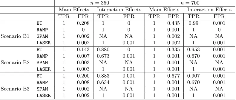
methods, we calculate the sum of squares error between the predicted response and the true response from the test set. These results are reported in Tables 1—3. In addition, we report in Appendix F the true and false positive rates for the main effects and interaction effects, defined as the proportion of correctly estimated active variables and the proportion of inactive variables that are incorrectly estimated to be active, respectively.

Seven approaches are compared in our numerical studies: our proposal,LASER; the sparse additive model,SpAM(Ravikumar et al., 2009); the nonparametric additive regression model with two-way interactions,VANISH(Radchenko and James, 2010); the backtracking method for modeling high-dimensional linear regression with two-way interaction terms, BT (Shah, 2016); the convex modeling of interactions with strong heredity,FAMILY(Haris et al., 2016); the regularization approach for high-dimensional quadratic regression, RAMP (Hao et al., 2018); the oracle approach by assuming that the active variables were known a priori,

ORACLE. In particular, the ORACLE is obtained by fitting nonparametric regression model

(14) using only the active variables with the ridge penalty for smoothness.

Our proposal LASER, SpAM, VANISH, and ORACLE are nonparametric. LASER involves fitting the nonparametric regression model (14) sequentially. In each step of Algorithm 1, we select the tuning parameter using a five-fold cross-validation on the training data set. Algorithm 1 is stopped when there is no more higher order interaction terms to be estimated. We fitLASERusing thekth basis expansion withk= 3. Note that the solution forSpAMcan be obtained from the first layer of LASER. ForVANISH, we simply use the default setting as in Radchenko and James (2010) and select the tuning parameter with cross-validation. For

ORACLE, we select the tuning parameter that yields the smallest sum of squares error on the

test set. In other words,ORACLEserves as a gold standard for nonparametric regression. The

FAMILY,RAMP, andBTare sparse high-dimensional linear regression with two-way interaction

terms. The tuning parameters for RAMP are selected using the extended BIC described in Hao et al. (2018). For FAMILY and BT, we consider a fine grid of tuning parameters and report the best results. In other words, we are giving unfair advantage toFAMILYand BT.

Most methods that estimate pairwise interaction terms are not computationally feasi-ble for high-dimensional profeasi-blem when d is large. Therefore, we consider both the low-dimensional and high-low-dimensional settings in Sections 5.1.1 and 5.1.2, respectively. We then perform numerical studies to assess how correlation among the covariates affects the performance of LASERin Section 5.1.3.

5.1.1 Low-Dimensional Setting with Two-Way Interactions

In our simulation studies, we generate∼N(0,1) and each element ofX from a uniform distribution on the interval [0,1]. We consider the following regression models with d= 30 covariates andn={200,400}:

A1 — A linear regression model with two-way interaction terms:

A2 — A non-linear regression model with two-way interaction terms (product of two indi-vidual functions):

f1(z) = √

2 [sin(6z)−0.0066], f2(z) = √

11[(2z−1)2−1/3], f3(z) =

√

12(z−1/2), f4(z) = √

16.6[exp(−5z)−0.2], f5(z) =

√

50[1/(1 +z)−0.69], y=

4

X

j=1

fj(xj) +f3(x1)f3(x2) +f5(x2)f4(x4) +f3(x3)f4(x4) + √

0.5,

where the constants are designed such that each function has mean zero and variance approximately one.

A3 — A non-linear regression model with two-way interaction terms (bivariate functions that cannot be decomposed as product of two individual functions):

y =

3

X

j=1

fj(xj) + √

19(√x1x2−4/9) + √

50[exp(−5x2x3)−0.438] + √

0.5,

where fj(xj) is as defined in Scenario A2.

The results, averaged over 200 data sets, are reported in Table 1.

Table 1: The sum of squares error (standard error) out of 200 test samples for the three different scenarios in Section 5.1.1, averaged over 200 data sets. The results are for models trained with ntraining samples. Numbers are rounded to the nearest integer.

Scenario A1 Scenario A2 Scenario A3

n= 200 n= 400 n= 200 n= 400 n= 200 n= 400 FAMILY 273 (2) 255 (2) 825 (10) 615 (7) 412 (3) 379 (3) BT 216 (1) 203 (2) 766 (14) 751 (13) 411 (3) 407 (3) RAMP 216 (2) 207 (2) 848 (21) 672 (22) 333 (9) 300 (9) SpAM 323 (3) 296 (2) 825 (10) 743 (10) 91 (1) 84 (1) VANISH 289 (3) 234 (2) 123 (3) 83 (1) 84 (1) 74 (1) LASER 279 (4) 226 (2) 124 (4) 84 (1) 75 (1) 63 (1) ORACLE 246 (2) 216 (2) 91 (1) 76 (1) 64 (1) 59 (1)

From Table 1, we see that BT and RAMP have the best performance in Scenario A1. This is not surprising since BT and RAMP are designed for modeling linear regression with two-way interaction terms. BothBTandRAMPoutperformFAMILYthat models the two-way interaction terms using a hierarchical penalty. For the nonparametric methods,SpAMhas the highest sum of squares error since the true model contains two-way interaction terms that

performance, and outperform SpAM. In summary, LASER is able to adaptively estimate the higher order terms accurately in both linear and non-linear regression settings.

5.1.2 High-Dimensional Setting with Three-Way Interactions

In this section, we consider the high-dimensional setting in which the number of variablesdis potentially larger than the number of observations. FAMILYandVANISHare computationally infeasible since there are a total ofd+ d₂

parameters and functions to estimate. Moreover, we consider settings with a three-way interaction effect to illustrate the flexibility of our proposal compared to existing methods such as BT and RAMP that are limited to modeling two-way interaction terms. We generate and X as in Section 5.1.1. We consider three regression models withd={200,400} covariates andn={350,700}:

B1 — A linear regression model with three-way interaction terms:

y=x1+x2+x3−2x1x2−2x1x3−2x2x3+ 25x1x2x3+ √

0.5.

B2 — A non-linear regression model with three-way interaction terms (product of individ-ual functions):

y= 3

X

j=1

fj(xj) +f3(x1)f3(x2) +f5(x2)f4(x3) +f1(x1)f4(x3) + 25(x1x2x3−1/8) + √

0.5,

wherefj(·) is as defined in Scenario A2.

B3 — A non-linear regression model with three-way interaction terms (bivariate functions that cannot be decomposed as product of two individual functions):

y= 3

X

j=1

fj(xj) +

√

19(√x1x2−4/9) + √

50[exp(−5x2x3)−0.438]

+f3(x1)f4(x3) + 25(x1x2x3−1/8) + √

0.5,

wherefj(·) is as defined in Scenario A2.

The results, averaged over 200 data sets, are reported in Table 2.

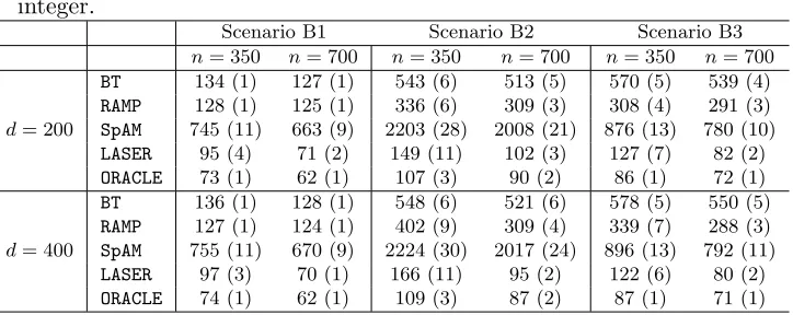
From Table 2, we see that LASER has the best performance across all scenarios since it is the only method that models the three-way interaction term. The sum of squares error is quite close to that of ORACLE even in the high-dimensional setting when n = 350 and

d= 400. As we increase the sample size, we see that the performance of LASER becomes more similar to that of ORACLE.

5.1.3 Two-Way Interactions With Correlated Data

In this section, we assess the performance of LASER when the covariatesX are correlated. We generate ∼ N(0,1) and X ∼ Nd(0,Σ), where Σjk = ρ|j−k| for 1 ≤ j, k ≤ d. For

Scenario C2, we normalize the covariates such that the observed values lie within the unit interval. We consider the following regression models with d = 30, n = 200, and ρ =

Table 2: The sum of squares error (standard error) out of 200 test samples for the three different scenarios in Section 5.1.2, averaged over 200 data sets. The results are for models trained with ntraining samples. Numbers are rounded to the nearest integer.

Scenario B1 Scenario B2 Scenario B3

n= 350 n= 700 n= 350 n= 700 n= 350 n= 700 BT 134 (1) 127 (1) 543 (6) 513 (5) 570 (5) 539 (4) RAMP 128 (1) 125 (1) 336 (6) 309 (3) 308 (4) 291 (3)

d= 200 SpAM 745 (11) 663 (9) 2203 (28) 2008 (21) 876 (13) 780 (10) LASER 95 (4) 71 (2) 149 (11) 102 (3) 127 (7) 82 (2) ORACLE 73 (1) 62 (1) 107 (3) 90 (2) 86 (1) 72 (1) BT 136 (1) 128 (1) 548 (6) 521 (6) 578 (5) 550 (5) RAMP 127 (1) 124 (1) 402 (9) 309 (4) 339 (7) 288 (3)

d= 400 SpAM 755 (11) 670 (9) 2224 (30) 2017 (24) 896 (13) 792 (11) LASER 97 (3) 70 (1) 166 (11) 95 (2) 122 (6) 80 (2) ORACLE 74 (1) 62 (1) 109 (3) 87 (2) 87 (1) 71 (1)

C1 — A linear regression model with two-way interaction terms:

y=x1+x6+x11+ 0.5x1x6−0.5x1x11+ 0.5x6x11+.

C2 — A non-linear regression model with two-way interaction terms:

y= 4

X

j=1

fj(xj) +f3(x1)f3(x6) +f5(x6)f4(x16) +f3(x11)f4(x16) + √

0.5,

where the fj(·) is as defined in Scenario A2.

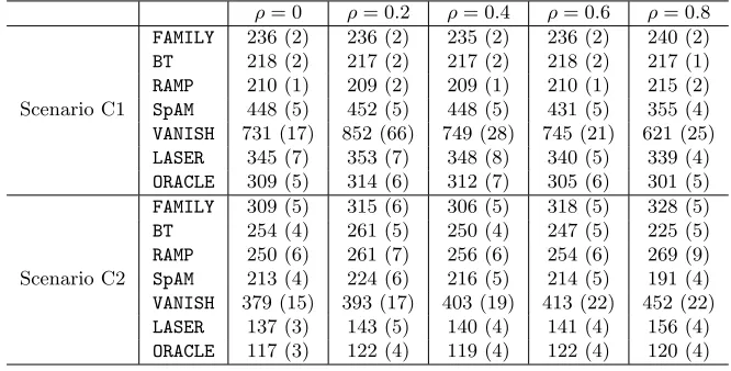
The results, averaged over 200 data sets, are reported in Table 3. From Table 3, we see that

LASER and ORACLEhave similar sum of squares error. Moreover, LASER outperforms SpAM

significantly. These results suggest that LASERis able to select the important main effects and interaction effects even when there are correlation among covariates.

5.2 Nonparametric Graphical Models

In this section, we perform some numerical studies to estimate nonparametric graphical models. We compare LASER to the graphical lasso (glasso) which estimate pairwise Gaussian graphical models (Friedman et al., 2008). We also consider the proposal of Liu et al. (2012) (kendall), a semiparametric approach for estimating nonparanormal graphical models. To evaluate the performance across different methods, we define the true positive rate as the proportion of correctly identified non-zeros, and the false positive rate as the proportion of zeros that are incorrectly identified to be non-zeros. In addition, we illustrate the main advantage of LASER in a stock price data by modeling three way cliques that quantify conditional dependencies among three variables, conditioned on the others.

Table 3: The sum of squares error (standard error) out of 200 test samples for the two scenarios in Section 5.1.3, averaged over 200 data sets. The results are for models trained with n = 200 training samples with d = 30 covariates. Numbers are rounded to the nearest integer.

ρ= 0 ρ= 0.2 ρ= 0.4 ρ= 0.6 ρ= 0.8 FAMILY 236 (2) 236 (2) 235 (2) 236 (2) 240 (2) BT 218 (2) 217 (2) 217 (2) 218 (2) 217 (1) RAMP 210 (1) 209 (2) 209 (1) 210 (1) 215 (2) Scenario C1 SpAM 448 (5) 452 (5) 448 (5) 431 (5) 355 (4) VANISH 731 (17) 852 (66) 749 (28) 745 (21) 621 (25) LASER 345 (7) 353 (7) 348 (8) 340 (5) 339 (4) ORACLE 309 (5) 314 (6) 312 (7) 305 (6) 301 (5) FAMILY 309 (5) 315 (6) 306 (5) 318 (5) 328 (5) BT 254 (4) 261 (5) 250 (4) 247 (5) 225 (5) RAMP 250 (6) 261 (7) 256 (6) 254 (6) 269 (9) Scenario C2 SpAM 213 (4) 224 (6) 216 (5) 214 (5) 191 (4) VANISH 379 (15) 393 (17) 403 (19) 413 (22) 452 (22) LASER 137 (3) 143 (5) 140 (4) 141 (4) 156 (4) ORACLE 117 (3) 122 (4) 119 (4) 122 (4) 120 (4)

studies to assess the performance of pairwise nonparametric graphical models using the score matching approach. More specifically, we consider two different simulation settings:

1. Gaussian graphical models: we simulate X ∼ N(0,Σ), where Σ is generated such that (Σ−1)jk = 0.4 for |k−j| = 1, (Σ−1)jj = 1, and setting the other elements to

zero.

2. Nonparametric graphical models: we simulate the data from the joint density

p(x)∝exp 

−

d

X

j=1 xj −

X

j<k

βjkx2jx2k



, (30)

where βjk = 1 for |k−j| = 1 and βjk = 0 otherwise. Noting that the conditional

distribution for each variable on the others is Gaussian, we employ a Gibbs sampler to simulate data from (30).

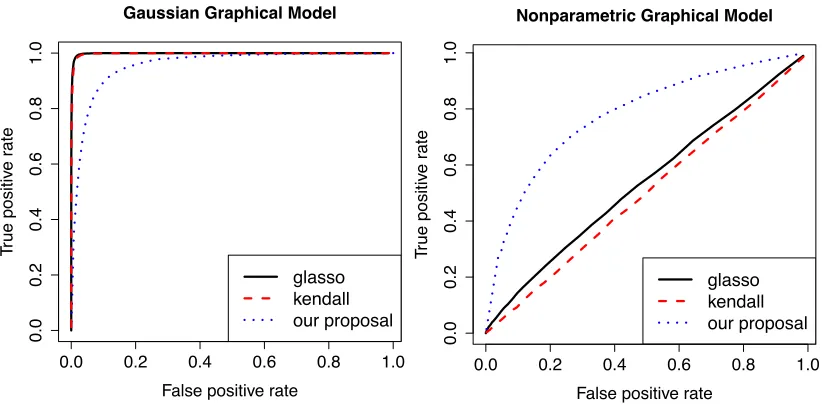
All of the aforementioned methods involve a sparsity tuning parameter. We applied a fine grid of tuning parameter values for all methods to obtain the curves in Figure 1. For Gaussian and nonparametric graphical models, we present results for n= 100 andp= 25, and n= 300 andp= 25, respectively. Results are averaged over 200 data sets.

0.0 0.2 0.4 0.6 0.8 1.0

0.0

0.2

0.4

0.6

0.8

1.0

Gaussian Graphical Model

False positive rate

Tr

ue positiv

e r

ate

glasso kendall our proposal

0.0 0.2 0.4 0.6 0.8 1.0

0.0

0.2

0.4

0.6

0.8

1.0

Nonparametric Graphical Model

False positive rate

Tr

ue positiv

e r

ate

glasso kendall our proposal

Figure 1: True and false positive rates, averaged over 200 data sets, for pairwise Gaussian and nonparametric graphical models. Left panel: Gaussian graphical models with

n= 100 and d= 25. The curves are obtained by varying the tuning parameter. Right panel: nonparametric graphical models withn= 300 andd= 25.

the joint density in (30) is clearly not multivariate Gaussian. Their performances are simi-lar to random guess even when we increasen by two-fold. LASER clearly outperforms the parametric approaches in this case. In conclusion, we sacrifice some performance in the parametric setting to gain flexibility in modeling nonparametric graphical models.

Next, we illustrate the main advantage of LASER by modeling three-way cliques that quantify conditional dependencies among three variables, conditioned on all of the other variables. To this end, we analyze the stock price data from Yahoo! Finance, which consists of daily closing prices for stocks in the S&P 500 index between January 1, 2003 and January 1, 2008. Stocks that are not consistently listed in the S&P 500 index during this time period are removed, leaving us withn= 1258 daily closing prices with 452 stocks. In this study, we categorize the stocks into six Global Industry Classification Standard sectors: Financials, Energy, Health Care, Information Technology, Materials, and Utilities.

The goal of our analysis is to understand the conditional dependence relationships among the six sectors. More specifically, we seek to learn the three-way conditional dependence relationships among thed= 6 sectors by modeling the three-way interaction terms in (17). Note that existing approaches for modeling graphical models in the literature are not able to model three-way cliques.

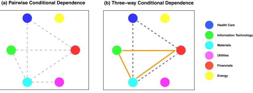
are conditionally dependent, given the other sectors. However, since we are estimating only the second order term at the second step of LASER, we cannot conclude that the three sectors financials, materials, and health care are jointly conditionally dependent.

To assess whether the three sectors are jointly conditionally dependent, we proceed to the next step of LASER for estimating three way interaction terms. We use the same tuning parameter to fit the model at the second step. The results are shown in Figure 2(b). Since the three way interaction term for health care, materials, and financials is estimated to be non-zero, we conclude that the three sectors are jointly conditionally dependent. Similar results hold for the sectors financials, materials, and information technology. Finally, LASER is terminated since there is no potential four way interaction terms to be estimated.

(a) Pairwise Conditional Dependence (b) Three−way Conditional Dependence

Health Care

Information Technology

Materials

Utilities

Financials

Energy

Figure 2: Estimated Conditional Dependence Graphs using the proposed method. Panel (a): Estimated pairwise conditional dependence relationships between two vari-ables, conditioned on the others. Panel (b): Estimated three-way conditional dependence relationships among three variables, conditioned on the others.

6. Discussion

In this paper, we propose a layer-wise learning strategy (LASER) for fitting multivariate function under the SSANOVA framework. LASER provides a computationally feasible framework for estimating SSANOVA models with higher order interaction effects. In addi-tion, we have shown that the estimators obtained from LASER is post-selection persistent. We illustrate LASER in the context of nonparametric regression and nonparametric graph-ical models problems. In the graphgraph-ical modeling literature, most work have focused on estimating pairwise graphical models, which corresponds to estimating the conditional de-pendence relationships between pairs of variables. LASER provides an alternative way to estimate conditional dependence relationships among a set of more than two variables. More generally, LASER can be easily applied to other problems that involves estimating multivariate function such as the generalized nonparametric regression.

two-way interaction effects are present. In this case, two-stage methods that perform variable screening on the main effects at the first stage, and then include the interaction effects based on the identified main effects may fail to identify some important covariates. To address this issue, Shah (2016) proposed a backtracking algorithm. The main idea is to first select a few variables that are most correlated with the response, and then include its corresponding interaction effects into the model. This process is repeated until no more variables are included in the model.

As a reviewer pointed out, the backtracking algorithm of Shah (2016) can be modified to accommodate higher order terms in the context of nonparametric regression. The main idea is as follows: (i) select a few univariate functions that are most highly predictive of the response by fitting the additive model for the main effects; (ii) include its associated two-way interaction effects, and subsequently the higher order interaction effects into the model; (iii) repeat (i) and (ii) until no more variables are included in the model. It is out of the scope of this paper to study such an extension carefully and we leave it for future work.

Acknowledgments

We thank two reviewers and the associate editor for providing helpful comments that im-proved the quality of this manuscript. We thank Peter Radchenko for providing R code to fit the model proposed in Radchenko and James (2010). This research is partially supported by the NSF DMS-1811315.

Appendix A. Proof of Theorem 1

Let S(r−1) _{be the support of}

b

f(r−1) and recall from (9) that conditional on the support

S(r−1)_,

b

f(r) _{is post-selection persistent if} R(fb(r))− inf

f∈F(r) R(f) =oP(1), where

F(r)₌

  

f :f(x) = X

J∈δ(S(r−1)₎

βJgJ(xJ),E[gJ] = 0,kgJkHJ ≤1,

X

J∈S(r−1)

β_J2+ X

J∈σ(S(r−1)₎

|βJ| ≤τ

  

.

For notational convenience, let f∗= arg inf_f∈F(r)R(f). The goal is to show thatR(fb(r))−

R(f∗) =oP(1).

Under the squared error loss, we define the risk R(f) and empirical riskRb(f) as

R(f) =E[(Y −f(X))2] and Rb(f) = 1

n n

X

i=1

(yi−f(xi))2,

respectively. By the definition of f∗, we have R(f∗) ≤ R(fb(r)). Thus, by the triangle inequality, we have

0≤R(fb(r))−R(f∗)≤R(fb(r))−Rb(fb(r)) +Rb(fb(r))−R(f∗) ≤ |R(fb(r))−Rb(fb(r))|+|Rb(f∗)−R(f∗)|

≤2 sup

f∈F(r)

|Rb(f)−R(f)|,

where the third inequality holds by the definition thatfb(r) is the minimizer ofRb(f), that is,Rb(fb(r))≤Rb(f∗). Thus, it suffices to obtain an upper bound on sup_f∈F(r)|Rb(f)−R(f)|.

Let J_r =δ(S(r−1)_{)∪ {∅}. With some abuse of notation, we write g}

J(xJ) =y when J

is an empty set. In addition, when f(x) = P

J∈δ(S(r−1)₎βJgJ(xJ), we also write the risk

function as R(β, g). Then, for any f ∈ F(r)_{, the risk and empirical risk can be rewritten as} R(β, g) = X

J,J0_∈J

r

βJβJ0_E[g_J(XJ)g_J0(X_J0)] andRb(β, g) = 1 n n X i=1 X

J,J0_∈J

r

βJβJ0g_J(x_iJ)g_J0(x_iJ0),

respectively. Thus, for all (β, g), we have

|Rb(β, g)−R(β, g)| ≤ X

J∈Jr

|βJ|

!2 max

J∈Jr

sup

gJ∈HJ,gJ0∈HJ0

(En−E)[gJgJ0],

whereEn[gJgJ0] =n−1Pn

i=1gJ(xiJ)gJ0(x_iJ0). Lets_r−1 be the cardinality of the setS(r−1).

We have

X

J∈Jr

|βJ|

!2 ≤2



 X

J∈S(r−1)

|βJ|

  2 + 2   X

J∈σ(S(r−1)₎

|βJ|





2

≤2sr−1



 X

J∈S(r−1)

β_J2





2

+ 2τ2 ≤(2sr−1+ 2)τ2,

(32)

where we use the inequality 2ab≤a2+b2 for anya >0 and b >0, and the constrained in the function class.

To obtain an upper bound, we begin with some notation. For a function class F and for any measureQ, the L∞ bracketing number N_{[ ]}(F, L∞(Q), ) is defined as the smallest number of pairs B = {(l1, u1), . . . ,(lk, uk)} such that kuj −ljk∞ ≤ for 1 ≤ j ≤ k, and

such that for everyf ∈ F, there exists (l, u)∈B such that l≤f ≤u. Define the function class

W ={gJgJ0 |g_J ∈ H_J, g_J0 ∈ H_J0,kg_Jk_H

J ≤1,kgJ0kHJ0 ≤1, J, J

0 _{∈ J}

r}. (33)

By Lemma 4, we have

logN_{[ ]}(W, L∞(Q), )≤C(rlogd+−r/m), (34) where C > 0 is some constant. By Corollary 19.35 of Van der Vaart (2000) and (34), we obtain

E max

J∈Jr

sup

gJ∈HJ,gJ0∈HJ0

(En−E)[gJgJ0]

! ≤ √C

n

Z C

0

q

logN_{[ ]}(W, L∞_{(Q), )d}

≤ √C

n

Z C

0

q

rlogd+−r/m_d

≤ √C

n

Z C

0

p

rlogd+−r/2md

≤C

r

rlogd n ,

where the third inequality follows from the fact that√a+b≤√a+√b, the last inequality follows from the assumption that r <2m, and C is a constant that may vary line to line.

By an application of Markov’s inequality, we have

max

J∈Jr

sup

gJ∈HJ,gJ0∈HJ0

(En−E)[gJgJ0] =O_P

r

rlogd n

!

. (36)

Combining the above with (32), we have that for all (β, g),

|Rb(β, g)−R(β, g)|=O_P 

τ2 s

rs2

r−1logd n



,

as desired.

Appendix B. Proof of Proposition 1

The proof of Proposition 1 is similar to that of the proof of Theorem 2 in Ravikumar et al. (2009). The main difference is that we have additional bivariate interaction terms in the true underlying model. Recall that S(1) _{is the support of the estimator obtained from solving}

(14) with r = 1. Recall from Section 3.1 that we approximate the main effects fj by its kth order basis expansion, i.e., fe_j =

Pk

l=1θljφjl(xj) =θjTφj(xj). Let θ∗j be the underlying

coefficients corresponding to the kth order basis expansion of the main effects. To simplify the notation, we let S= ¯S(1)_.

Let ΦS be the n×k|S| matrix with rows φS(x1), . . . ,φS(xn), where φS(·) is obtained

by concatenating φj(·) for all j ∈ S. Similarly,θS∗ is obtained by concatenatingθ∗j for all j ∈ S. Recall that we denote the projection operator PS¯(2)f =

P

(s,t)∈S¯(2)fst. We now

consider a second order Taylor expansion offst at (1/2,1/2) for each (s, t)∈S¯(2): fst(xs, xt) =fst(0.5,0.5) +

X

j∈{s,t}

∂xjfst(0.5,0.5)(xj−0.5) +

1 2∂

2

xjfst(0.5,0.5)(xj−0.5)

2

+∂_x2_sxtfst(0.5 +η(xs−0.5),0.5 +η(xt−0.5))(xs−0.5)(xt−0.5), (37)

where η ∈ [0,1]. Since ΦS is the design matrix generated from B-spline polynomials, we

can represent the vector u := (PS¯(2)f(x1), . . . , PS¯(2)f(xn))T as u =ΦSγS∗ + ∆, where the ith entry of ΦSγS∗ represents the leading terms in (37) and γS∗ is the corresponding basis

coefficients vector:

[ΦSγS∗]i=P(s,t)∈_S¯(2)

fst(0.5,0.5)+Pj∈{s,t}(∂xjfst(0.5,0.5)(xij−0.5)+ 1 2∂

2

xjfst(0.5,0.5)(xij−0.5) 2₎

.

The remainder ∆ corresponds to the last term in (37), i.e., for eachi= 1, . . . , n,

∆i=P_(s,t)∈S¯(2)∂_x2_sxtfst(0.5 +η(xis−0.5),0.5 +η(xit−0.5))(xis−0.5)(xit−0.5).

Thus,k∆k∞≤q∗n, whereq∗n:=k

P

(s,t)∈S¯(2)∂2_xsxtfstk∞.

Denote ΣSS = _n1ΦT_SΦS. Let = (1, . . . , n)T, and let v =y−ΦS(θ_S∗ +γ_S∗)−∆−

Theorem 2 in Ravikumar et al. (2009), we have an additional term ∆. Therefore, following the same proof, we have

kθb_S−θ_S∗ −γ_S∗k_∞≤

Σ−_SS1 1 nΦ T S ∞ +

Σ−_SS1

1

nΦ T

S(v+ ∆)

∞

+λkΣ−_SS1bgSk∞, (38)

where θS and bgS are subvectors of the estimator in (14) for r = 1 and the gradient of the penalty in (14) forr = 1, respectively. If we can show that

kθb_S−β_S∗k∞<

1

2minj∈Skθ ∗

j +γj∗k∞=

1

2minj∈S kβ ∗

jk∞=ρ∗n,

then kθb_jk∞>0 for eachj ∈S, i.e., S(1) ⊇S. Therefore, it suffices to show that the right

hand side of (38) is smaller than ρ∗_n. Compared to the right hand side of Equation (83) in Ravikumar et al. (2009), we only have an additional termkΣ−_SS1(_n1ΦT_S∆)k∞ in (38).

Since k∆k∞ ≤ q∗n, we can bound kΣ −1 SS(

1 nΦ

T

S∆)k∞ following the same procedure as kΣ−_SS1(_n1ΦT_Sv)k∞. According to Equations (99) and (111) in Ravikumar et al. (2009), if p

|S¯(1)_|kq∗

n/ρ∗n=o(1) and √

kq_n∗/λ=o(1), terms related to ∆ will be dominated by terms related to and v, and the remaining proof in Ravikumar et al. (2009) follows through.

Appendix C. Proof of Lemma 1

Recall from Section 4.3 that we define r0(x) to be the element-wise differentiation of the vectorr(x). Also, recall from (22) that the modified Fisher divergence is defined as

1 2

Z

[0,1]d

p(x)kr(x)◦[∇logp(x)− ∇logq(x)]k2₂dx=T1+T2+T3, where (39)

T1 =

1 2

Z

[0,1]d

p(x)kr(x)◦ ∇logq(x)k2 2dx, T2 =−

Z

[0,1]d

p(x) (r(x)◦ ∇logp(x))T (r(x)◦ ∇logq(x))dx,

T3 =

1 2

Z

[0,1]d

p(x)kr(x)◦ ∇logp(x)k2₂dx.

By some algebraic manipulation, we have

T2=−

Z

[0,1]d

p(x) (r(x)◦ ∇logp(x))T (r(x)◦ ∇logq(x))dx

=− Z

[0,1]d

(∇p(x))T(r(x)◦r(x))◦ ∇logq(x)dx

=

d

X

j=1

"

−p(x)∇jlogq(x)r2j(xj)

1 0+ Z [0,1]d

p(x) ∂

∂xj

r_j2(xj)∇jlogq(x) dx

#

= Z

[0,1]d

p(x)h 2r(x)◦r0(x)T