ROBERT COSTANZA
Center for Environmental and Estuarine Studies
Zoology Department and Institute for Ecological Economics University of Maryland, Box 38
Solomons, Maryland 20688-0038, USA
MATTHIAS RUTH*
Center for Energy and Environmental Studies Boston University
675 Commonwealth Ave.
Boston, Massachusetts 02215, USA
ABSTRACT / This paper assesses the changing role of dy-namic modeling for understanding and managing complex ecological economic systems. It discusses new modeling
tools for problem scoping and consensus building among a broad range of stakeholders and describes four case stud-ies in which dynamic modeling has been used to collect and organize data, synthesize knowledge, and build consensus about the management of complex systems. The case stud-ies range from industrial systems (mining, smelting, and re-fining of iron and steel in the United States) to ecosystems (Louisiana coastal wetlands, and Fynbos ecosystems in South Africa) to linked ecological economic systems (Mary-land’s Patuxent River basin in the United States). They illus-trate uses of dynamic modeling to include stakeholders in all stages of consensus building, ranging from initial problem scoping to model development. The resultant models are the first stage in a three-stage modeling process that includes research and management models as the later stages.
Types and Uses of Models
In environmental systems, nonlinearities and spatial and temporal lags prevail. However, all too often these system features are moved to the sidelines of scientific investigations. As a consequence, the presence of nonlin-earities and spatial and temporal lags significantly reduces the ability of these investigations to provide insights that are necessary to make proper decisions about the management of complex ecological–eco-nomic systems. New modeling approaches are required to effectively identify, collect, and relate the informa-tion that is relevant for understanding those systems, to make consensus building an integral part of the model-ing process, and to guide management decisions.
Model building is an essential prerequisite for com-prehension and for choosing among alternative actions. Humans build mental models in virtually all decision situations, by abstracting from observations that are deemed irrelevant for understanding that situation and by relating the relevant parts with each other. Language itself is an expression of mental modeling, and one could argue that without modeling there could be no
rational thought at all. For many everyday decisions, mental models are sufficiently detailed and accurate to be reliably used. Our experiences with these models are passed on to others through verbal and written accounts that frequently generate a common group understand-ing of the workunderstand-ings of a system.
In building mental models, humans typically simplify systems in particular ways. We base most of our mental modeling on qualitative rather than quantitative relation-ships, we linearize the relationships among system components, disregard temporal and spatial lags, treat systems as isolated from their surroundings or limit our investigations to the system’s equilibrium domain. When problems become more complex, and when quantita-tive relationships, nonlinearities, and time and space lags are important, we encounter limits to our ability to properly anticipate system change. In such cases, our mental models need to be supplemented.
Statistical approaches based on historical or cross-sectional data often are used to quantify the relation-ships among system components. To be able to deal with multiple feedbacks among system components and with spatial and temporal lags requires the availability of rich data sets and elaborate statistical models. Recent advances in statistical methods have significantly im-proved the ability to test for the goodness of fit of alternative model specifications and have even at-tempted to test for causality in statistical models (Granger 1969, 1993). Typically, little attention is given to first principles in attempts to use statistical models to
KEY WORDS: Dynamic modeling; Scoping; Consensus building; En-vironmental management; Ecosystem management; Policy making; Graphical programming languages
*Author to whom correspondence should be addressed.
arrive at a better understanding of the cause-effect relationships that lead to system change. Model results are driven by data, the convenience of estimation techniques, and statistical criteria—none of which en-sure that the fundamental drivers for system change are satisfactorily identified (Leontief 1982, Leamer 1983). By the same token, a statistical modeling exercise can only provide insight into the empirical relationships over a system’s history or at a point in time, but it is of limited use for analyses of a system’s future develop-ment path under alternative managedevelop-ment schemes (Allen 1988). In many cases, those alternative manage-ment schemes include decisions that have not been chosen in the past, and their effects are therefore not captured in the data of the system’s history or present state.
Dynamic modeling is distinct from statistical model-ing by buildmodel-ing into the representation of a phenom-enon those aspects of a system that we know actually exist—such as the physical laws of material and energy conservation that describe input–output relationships in industrial and biological processes (Hannon and Ruth 1994, 1997). Dynamic modeling therefore starts with an advantage over the purely statistical or empirical modeling schema. It does not rely on historic or cross-sectional data to reveal those relationships. This advantage also allows dynamic models to be used in more related applications than empirical models— dynamic models are more transferable to new applica-tions because the fundamental concepts on which they are built are present in many other systems.
Computers have come to play a large role in develop-ing dynamic models for decision-makdevelop-ing support in complex systems. Their ability to numerically solve for complex nonlinear relationships among system compo-nents and to deal with time and space lags and disequi-librium conditions make obsolete the use of linear functional relationships or restriction of the analysis to equilibrium points.
It is inappropriate to think of models as anything but crude—yet in many cases absolutely essential—abstract representations of complex interrelationships among system components (Levins 1966, Robinson 1991, Ruth and Cleveland 1996). Their usefulness can be judged by their ability to help solve decision problems as the dynamics of the real system unfold (Ruth and Hannon 1997). The dynamic models presented in this paper are designed with that criterion in mind. They are interac-tive tools that reflect the processes that determine system change and respond to the choices made by a decision maker.
Models are essential for policy evaluation, but, unfor-tunately, they can also be misused since there is ‘‘. . . the
tendency to use such models as a means of legitimizing rather than informing policy decisions. By cloaking a policy decision in the ostensibly neutral aura of scien-tific forecasting, policy-makers can deflect attention from the normative nature of that decision . . .’’ (Robin-son 1993). The misguided quest for objective model building highlights the need to recognize, and more effectively deal with, the inherent subjectivity of the model development process. In this paper we wish to put computer modeling in its proper perspective: as an inherently subjective but absolutely essential tool useful in supplementing our existing mental modeling capabili-ties in order to make more informed decisions, both individually and in groups.
In the case of modeling ecological and economic systems, purposes can range from developing simple conceptual models, in order to provide a general understanding of system behavior, to detailed realistic applications aimed at evaluating specific policy propos-als. It is inappropriate to judge this whole range of models by the same criteria. At minimum, the three criteria of realism (simulating system behavior in a qualitatively realistic way), precision (simulating behav-ior in a quantitatively precise way), and generality (representing a broad range of systems’ behaviors with the same model) are necessary (Holling 1964, Levins 1966). No single model can maximize all three of these goals, and the choice of which objectives to pursue depends on the fundamental purposes of the model.
In this paper we propose a three-step process for developing computer models of a situation that begins with an initial scoping and consensus-building stage aimed at producing simplified, high generality models, and then moving to a more realistic research modeling stage, and only then coming to a high precision manage-ment model stage. We elaborate this process further on.
Using Models to Build Consensus
decisions on environmental investments and problems is key to achieving fairness and sustainability (Rawls 1971, 1987).
Integrated modeling of large systems, from indi-vidual companies to industries to entire economies or from watersheds to continental-scale systems and ulti-mately to the global scale, requires input from a very broad range of people. We need to see the modeling process as one that involves not only the technical aspects, but also the sociological aspects involved with using the process to help build consensus about the way the system works and which management options are most effective. This consensus needs to extend both across the gulf separating the relevant academic disci-plines and across the even broader gulf separating the science and policy communities, and the public. Appro-priately designed and approAppro-priately used modeling exercises can help us bridge these gulfs.
The process of modeling can (and must) serve this consensus building function. It can help to build mutual understanding, solicit input from a broad range of stakeholder groups, and maintain a substantive dialog between members of these groups. Modeling and consensus building are essential components in the process of adaptive management (Gunderson and oth-ers 1995).
Modeling Tools for Scoping
and Consensus Building
Various forms of computer models for scoping and consensus building have been developed for business management applications (Roberts 1978, Lyneis 1980, Westenholme 1990, 1994, Morecroft and others 1991, Vennix and Gubbels 1994, Morecroft and van der Heijden 1994, Senge and Sterman 1994). While previ-ous emphasis was placed on the provision of computer hardware and software to support group communica-tion (Kraemer and King 1988), recent trends are to facilitate problem structuring methods and group deci-sion support (Checkland 1989, Rosenhead 1989, Phill-ips 1990). The use of computers to structure problems and provide group decision support has been spurred by the recognition that in complex decision settings bounds on human rationality can create persistent judgment biases and systematic errors (Simon 1956, 1979, Kahnemann and Tversky 1974, Kahnemann and others 1982, Hogarth 1987). To identify relevant infor-mation sources, assess relationships among decisions, actions and results, and hence to facilitate learning requires that cause and effect are closely related in space and time. Dynamic modeling is one such tool that
helps us close spatial and temporal gaps between decisions, actions, and results.
Dynamic modeling has increasingly become a part of executive debate and dialog to help avoid judgment biases and systematic errors in business management decision making (Senge 1990, Morecroft 1994). It has also penetrated, albeit to a lesser extent, the assessment of environmental investments and problems (Ruth 1993). Both areas of application of dynamic modeling have significantly benefited from the use of graphical programming languages. One of the main strengths of these programming languages is to enable scientists and decision makers to focus and clarify the mental model they have of a particular phenomenon, to augment this model, elaborate it, and then to do something they cannot otherwise do: run the model and let it yield the inevitable dynamic consequences hidden in their as-sumptions and their understanding of a system. With their relative ease of use, these graphical programming languages offer powerful tools for intellectual inquiry into the workings of complex ecological–economic systems (Hannon and Ruth 1994, 1997).
To model and better understand nonlinear dynamic systems requires that we describe the main system components and their interactions. System components can be described by a set of state variables—or stocks— such as the capital stock in an economy or the amount of sediment accumulated on a landscape. These state variables are influenced by controls—or flows—such as annual investment in new capital or seasonal sediment fluxes. The extent of the controls—the size of the flows—in turn may depend on the stocks themselves and other parameters of the system.
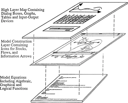
There are various graphical programming languages available that are specifically designed to facilitate modeling of nonlinear, dynamic systems. Among the most versatile of these languages is the graphical pro-gramming language STELLA (Costanza 1987, Rich-mond and Peterson 1994, Hannon and Ruth 1994). STELLA runs in the Macintosh and Windows environ-ments. A STELLA dynamic systems model consists of three communicating layers that contain progressively more detailed information on the structure and func-tioning of the model (Figure 1). The high-level map-ping and input-output layer provides tools to lay out the structure of the model and to enable non-modelers to easily grasp that structure, to interactively run the model and to view and interpret its results. The ease of use of the model at this aggregate level of detail thus enables individuals to become intellectually and emo-tionally involved with the model (Peterson 1994).
and connected with each other. STELLA represents stocks, flows and parameters, respectively, with the following three symbols:
Icons can be selected and placed on the computer screen to define the main building blocks of the computer model. The structure of the model is estab-lished by connecting these symbols through ‘‘informa-tion arrows’’
Once the structure of the model is laid out on the screen, initial conditions, parameter values, and func-tional relationships can be specified by simply clicking on the respective icons. Dialog boxes appear that ask for the input of data or the specification of graphically or mathematically defined functions.
Equally easy is the generation of model output in tabular or graphical form through the choice of icons. With the use of sliders, a user can also immediately respond to the model output by choosing alternative parameter values as the model runs. Subsequent runs under alternative parameter settings and with different responses to model output can be plotted in the same graph or table to investigate the implications of alterna-tive assumptions. Thus, the modeling approach is not only dynamic with respect to the behavior of the system itself but also with respect to the learning process that is initiated among decision makers as they observe the system’s dynamics unfold. The process of learning by doing experiments on the computer rather than in the real world gives model users the opportunity to investi-gate the implications of their assumptions for the
system’s dynamics and to assess their ability to make the right decision under alternative assumptions.
The lowest layer of the STELLA modeling environ-ment contains a listing of the graphically or algebra-ically defined relationships among the system compo-nents together with initial conditions and parameter values. These equations are solved in STELLA with numerical techniques. The equations, initial condi-tions, and parameter values can also be exported and compiled to conduct sophisticated statistical analyses and parameter tests (Oster 1996) and to run the model on various computing platforms (Costanza and others 1990, Costanza and Maxwell 1993).
A Three-Step Modeling Process
To support decisions on environmental investments and problems, we advocate the use of a three-step modeling process. The first stage is to develop a high-generality, low-resolution scoping and consensus building model involving broad representation of stake-holder groups affected by the problem. STELLA and similar software make it feasible to involve a group of relative modeling novices in the construction of rela-tively complex models, with a few people competent in modeling acting as facilitators. Using STELLA, and projecting the computer screen onto the wall or sharing a model via the internet, the process of model construc-tion can be transparent to a group of diverse stakehold-ers. Participants can follow the model construction process and contribute their knowledge to the process. After the basic model structure is developed, the program requires more detailed decisions about the functional connections between variables. This process is also transparent to the group, using well-designed dialog boxes and the potential for graphic and alge-braic input. The models that result from this process are designed to capture as much realism as possible and to answer preliminary questions about system dynamics, especially its main areas of sensitivity and uncertainty, and thus to guide the research agenda in the following modeling stage.
The second-stage research models are more detailed and realistic attempts to replicate the dynamics of the particular system of interest. This stage involves collect-ing large amounts of historical data for calibration and testing and a detailed analysis of the areas of uncertainty in the model. It may involve traditional ‘‘experts’’ and is more concerned with analyzing the details of the historical development of a particular system with an eye toward developing specific scenarios or policy op-tions in the next stage. It is still critical to maintain stakeholder involvement and interaction in this stage
through the exchange of models and with regular workshops and meetings to discuss model progress and results.
While integrated models aimed at realism and preci-sion are large, complex, and loaded with uncertainties of various kinds (Costanza and others 1990, Groffman and Likens 1994, Bockstael and others 1995), our abilities to understand, communicate, and deal with these uncertainties are rapidly improving. It is also important to remember that while increasing the resolu-tion and complexity of models increases the amount we can say about a system, it also limits how accurately we can say it. Model predictability tends to fall with increas-ing resolution due to compoundincreas-ing uncertainties (Cos-tanza and Maxwell 1993). What we are after are models that optimize their effectiveness (Costanza and Sklar 1985) by choosing an intermediate resolution where the product of predictability and resolution (effective-ness) is maximized. As a consequence, resolution of the research models is medium to high, depending on the results of the scoping model.
The third stage of management models is focused on producing scenarios and management options in this context of adaptive feedback and monitoring and is based on the earlier scoping and research models. It is also necessary to place the modeling process within the larger framework of adaptive management (Holling 1978) if management is to be effective. Adaptive ment views regional development policy and manage-ment as experimanage-ments, where interventions at several scales are made to achieve understanding and to iden-tify and test policy options (Holling 1978, Walters 1986, Lee 1993, Gunderson and others 1995). This means that models and policies based on them are not taken as the ultimate answers, but rather as guiding an adaptive experimentation process with the regional system. Em-phasis is placed on monitoring and feedback to check and improve models, rather than using models to obfuscate and defend a policy that is not corresponding to reality. Continuing stakeholder involvement is essen-tial in adaptive management.
Each of these stages in the modeling process has useful products, but the process is most beneficial and effective if followed in the order described. Too often we jump to the research or management stage of the process without first building adequate consensus about the nature of the problem and without involving the appropriate stakeholder groups. What we save in time and effort by jumping ahead is easily lost later on in attempts to forge agreement about results and generate compliance with the policies derived from the model.
Case Studies
In this section we briefly describe a set of case studies that embody some or all of the characteristics of the three-stage modeling process outlined above. The pur-pose of this section is to illustrate the wide range of environmental issues to which scoping and consensus building modeling has been applied and to indicate the various degrees to which stakeholder involvement has been achieved in model development. We begin with case studies that solicited from stakeholders specific information to be included in the models and that shared throughout the modeling process the models with the contributors through a series of conversations, mailings and presentations. We also present examples of cases in which workshop meetings for scoping and consensus building have been conducted and a group of stakeholders convened to collectively develop models for scoping and consensus building purposes. Some of the models presented here have been followed up with more detailed research and management models.
US Iron and Steel Production
The iron and steel industry is the single largest energy consumer in the industrial sector of the US economy and is characterized by large-scale operations that require significant capital investment to change their structure and functioning. The high degree of interconnectedness among the various production stages often requires technological adjustments at one stage in response to change elsewhere in the industry. For example, many vertically integrated steel plants have been retiring their coke ovens, replacing them with imported coke, and decreasing the production of pig iron, in which coke is used to reduce iron ores. The decline in pig iron production from blast furnaces is accompanied by a shift in raw steel production technolo-gies away from those that use pig iron as their main input if overall raw steel output is to be maintained (Sparrow 1983, Ross 1987, Ruth 1995). This typically means movement towards electric arc furnaces, whose main energy input is electricity.
One consequence of the changes in technologies at the various production stages is a significant change in the industry’s energy-use profile. By-products such as coke oven gas and blast furnace gas have traditionally been used as energy sources in basic oxygen furnaces. The reduced production of pig iron leads to an increase in the fractions of energy purchased elsewhere rather than produced by the industry itself. The latter affects the industry’s influence on its supply and cost of energy and has ramifications for its emissions profile.
implementation of new technologies and the many interdependencies among the various production stages make it necessary for decision makers to anticipate long-term trends in demand for the industry’s products and supply of raw materials and energy. By the same token, to move towards sustainable industry practices requires managers and policy decision makers to ex-plore the implications for the industry’s material and energy-use profiles under a wide range of scenarios about changes in demand and the speed at which technologies can be adapted (Ruth and Harrington 1997).
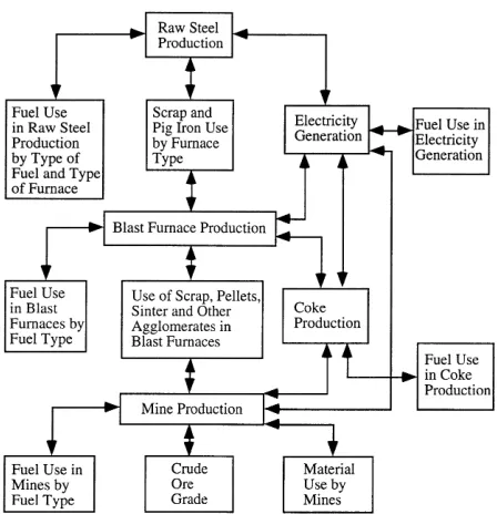
Using STELLA software, a model has been devel-oped of iron ore mining, processing, and raw steel production for the aggregate US iron and steel industry with the goal to identify the industry’s future likely profiles of material and energy use. The goal of the scoping and consensus building modeling of US iron and steel industries was to capture the feedbacks among various production stages in the industry in terms of material and energy use. Particular attention was given to changes in material and energy flows in response to changes in input materials, technical change at the various production stages, and changes in demand for raw steel (Weston and Ruth 1997). A series of informal, iterative interviews with industry experts, members of industry associations, and consultants was carried out to arrive at a model structure that is sufficiently detailed to capture the various feedbacks and sufficiently simple to be easily communicated to nonexpert modelers. Signifi-cant agreement was already present at the outset of the model development process on the system boundaries that define the respective production stages and on the key material and energy types to be included in the model. Based on this consensus, the model captures mining, pig iron and raw steel production, and modules for electricity generation and coke production (Figure 2).
To generate consensus on the specification of mate-rial and energy use at the various production stages and the feedback processes that occur among them, engi-neering information from various sources was used and supplemented with time series data derived from pub-lished sources. These quantifications provided a bench-mark for model runs. To explore industry’s profiles of material and energy use under alternative assumptions, the model was set up to be run in an interactive modeling mode that enables decision makers to choose different parameter settings based on their understand-ing of the industry. Additionally, the model was de-signed to investigate the implications that various rates of change in demand for the industry’s products and in technologies may have on material and energy use at
individual production stages and by the industry as a whole.
The discussions with industry experts prior to setting up the model and running it indicated a prevailing assumption that even though crude ore reserves are finite, absolute amounts are large and ore grades sufficiently high to not pose a constraint on industry in the long run. Various model runs refuted this view of the industry. The model indicates over a wide range of reasonable assumptions that, although there is no shortage of iron ore in the United States, declines in ore grade lead to increases in total energy consumption per ton of raw steel output that is unlikely to be compen-sated for by improvements in technology—even in the presence of further increased recycling rates and only moderate demand increases. Valuable insight was gener-ated with regard to changes in the industry’s energy mix, technology mix, and the time frames in which these changes are likely to occur.
Subsequently, the model has been significantly ex-tended from the model designed for scoping and consensus building to include indirect energy require-ments by the iron and steel industry and direct and indirect carbon emissions (Ruth 1995). Efforts are under way to work with managers in industry to guide investment decisions at the level of the firm and provide management support. Similar applications of dynamic modeling to industrial processes have been conducted for several other metals industries (Ruth 1997), US pulp and paper production (Ruth and Harrington 1997),
and US glass production for containers, flat glass, and fiberglass (Ruth and Dell’Anno 1997).
Louisiana Coastal Wetlands
Applications of dynamic modeling to scoping and consensus building in industrial systems have concen-trated on material and energy flows within these systems and between these systems and their environment. In contrast, the Louisiana coastal wetlands project traces the distribution of water and sediment through a landscapes.
The changing historical sequence of Mississippi River main distributaries have deposited sediments to form the current Mississippi deltaic plain marshes. This delta switching cycle lasts on average 1500 years and sets the historical context of this landscape. At present, the river is in the process of changing from the current channel to the much shorter Atchafalaya River. The US Army Corps of Engineers maintains a control structure at Old River to control the percentage of Mississippi River flow going down the Atchafalaya. Since about 1950 this percentage has been set at approximately 30%. Atchafa-laya River-borne sediment first filled in open water areas in the upper Atchafalaya basin, and more recently has begun to build a delta in Atchafalaya Bay (Roberts and others 1980, Van Heerden and Roberts 1980a,b). Dur-ing the next few decades, a new delta is projected to form at the mouth of the river, and plant community succession will occur on the recently formed delta and in the existing marshes. At the same time, the overall Louisiana coastal zone is projected to have a net loss of approximately 100 km2/yr due to sediment starvation
and salt water intrusion (Gagliano and others 1981). The leveeing of the Mississippi and Atchafalaya rivers, along with the damming of distributaries, has virtually eliminated riverine sediment input to most Louisiana coastal marshes. This change has broken the deltaic cycle and greatly accelerated land loss. Only in the area of the Atchafalaya delta is sediment-laden water flowing into wetland areas and land gain occurring (Roberts and others 1980, Van Heerden and Roberts 1980a,b).
Primary human activities that potentially contribute to wetland loss are flood control, canals, spoil banks, land reclamation, fluids withdrawal, and highway con-struction. There is evidence that canals and levees are an important factor in wetland loss in coastal Louisiana, but there is much disagreement about the magnitude of the indirect loss caused by them (Craig and others 1979, Cleveland and others 1981, Scaife and others 1983, Deegan and others 1984, Leibowitz 1989). Natural channels are generally not deep enough for the needs of oil recovery, navigation, pipelines, and drainage, so a
vast network of canals has been built. In the deltaic plain of Louisiana, canals and their associated spoil banks of dredged material currently comprise 8% of the total marsh area compared to 2% in 1955. The construc-tion of canals leads to direct loss of marsh by dredging and spoil deposition and indirect loss by changing hydrology, sedimentation, and productivity. Canals are thought to lead to more rapid salinity intrusion, causing the death of freshwater vegetation. Canal spoil banks also limit water exchange with wetlands, thereby decreas-ing deposition of suspended sediments.
Proposed human activities can have a dramatic impact on the distribution of water and sediments from the Atchafalaya River and consequently on the develop-ment of the Atchafalaya landscape. For example, the Corps of Engineers was considering extending a levee along the east bank of the Atchafalaya that would restrict water and sediment flow into the Terrebonne marshes.
This situation represented both a unique nity to study landscape dynamics and a unique opportu-nity to build consensus about how the system works and how to manage it. The Atchafalaya landscape is chang-ing rapidly enough to provide time-series observations that can be used to test basic hypotheses about how coastal landscapes develop. In addition to short-term observations, there is a uniquely long and detailed history of field and remotely sensed data available on the study area (Bahr and others 1983, Costanza and others 1983). Solutions to the land loss problem in Louisiana all have far-reaching implications. They de-pend on which combination of solutions are under-taken and when and where they are underunder-taken. Out-side forces (such as rates of sea level rise) also influence the effectiveness of any proposed solution. In the past, suggested solutions have been evaluated independently of each other, in an ad hoc manner, and without adequate dialog and consensus among affected parties. In order to address this problem in a more compre-hensive way, a project was started in 1986 to apply the three-stage modeling approach described above. The first stage of scoping and consensus building involved mainly representatives of the Corps of Engineers, the US Fish and Wildlife service, local landowners and environmentalists, and several disciplines within the academic community. This stage involved a series of workshops aimed at developing a unit model, using STELLA, of the basic processes occurring at any point in the landscape, and at coming to agreement about how to model the entire landscape in the later stages. This stage took about a year.
(Cos-tanza and others 1988, 1990, Sklar and others 1985, 1989) that replicated the unit model developed in stage 1 over the coastal landscape and added horizontal flows of water, nutrients, and sediments, along with succes-sional algorithms to model changes in the distribution pattern of habitats on the landscape. Using this ap-proach, the ability was demonstrated to simulate the past behavior of the system in a fairly realistic way (Costanza and others 1990). This part of the process took about three years.
In the third (management) stage of the dynamic modeling process, a range of projected future condi-tions was laid out as a function of various management alternatives and natural changes, both individually and in various combinations. The research and manage-ment model simulates both the dynamic and spatial behavior of the system, and it keeps track of several of the important landscape-level variables in the system, such as ecosystem type, water level and flow, sediment levels and sedimentation, subsidence, salinity, primary production, nutrient levels, and elevation.
The research and management model was called the Coastal Ecological Landscape Spatial Simulation (CELSS) model. It consists of 2479 spatial cells of 1-km2
to simulate a rapidly changing section of the Louisiana coast and predict long-term (50- to 100-year) spatially articulated changes in this landscape as a function of various management alternatives and natural and hu-man-influenced climate variations.
The model was run on a Cray supercomputer from initial conditions in 1956 through 1978 and 1983 (years for which additional data were available for calibration and validation) and on to the year 2033 with a maxi-mum of weekly time steps. It accounted for 89.6% of the spatial variation in the 1978 calibration data and 79% of the variation in the 1983 verification data. Various future and past scenarios were analyzed with the model, including the future impacts of various Atchafalaya River levee extension proposals, freshwater diversion plans, marsh damage mitigation plans, future global sea-level rise, and the historical impacts of past human activities and past climate patterns.
The model results were used by the Corps of Engi-neers and the Fish and Wildlife Service in making decisions about these management options. Because they were involved directly as participants in the process through all three stages, the model results were much easier to communicate and implement. The partici-pants also had a much more sophisticated understand-ing of the underlyunderstand-ing assumptions, uncertainties, and limitations of the model, along with its strengths, and could use it effectively as a management tool.
South African Fynbos Ecosystems
While the Louisiana wetlands project concentrated on aspects of the physical landscape, a scoping and consensus-building project was initiated to address is-sues of species diversity. The area of study is the Cape Floristic Region—one of the world’s smallest and, for its size, richest floral kingdoms. This tiny area, occupying a mere 90,000 km2, supports 8500 plant species of which
68% are endemic, 193 endemic genera, and six en-demic families (Bond and Goldblatt 1984). Because of the many threats to this region’s spectacular flora, it has earned the distinction of being the world’s hottest hot-spot of biodiversity (Myers 1990).
The predominant vegetation in the Cape Floristic Region is fynbos, a hard-leafed and fire-prone shrub-land that grows on the highly infertile soils associated with the ancient, quartzitic mountains (mountain fyn-bos) and the wind-blown sands of the coastal margin (lowland fynbos) (Cowling 1992). Owing to the preva-lent climate of cool, wet winters and warm, dry sum-mers, fynbos is superficially similar to California chapar-ral and other Mediterranean climate shrublands of the world (Hobbs and others 1995). Fynbos landscapes are extremely rich in plant species (the Cape Peninsula has 2554 species in 470 km2) and narrow endemism ranks
among the highest in the world (Cowling and others 1992).
In order to adequately manage these ecosystems several questions had to be answered, including, what services do these species-rich fynbos ecosystems provide and what is their value to society? A two-week workshop was held at the University of Cape Town (UCT) with faculty and students from different disciplines along with parks managers, business people, and environmen-talists. The primary goal of the workshop was to pro-duce a series of consensus-based research papers that critically assessed the practical and theoretical issues surrounding ecosystem valuation as well as assessing the value of services derived by local and regional communi-ties from fynbos systems.
To achieve the goals, an atelier approach was used to form multidisciplinary, multicultural teams, breaking down the traditional hierarchical approach to problem-solving. Open space (Rao 1994) techniques were used to identify critical questions and allow participants to form working groups to tackle those questions. Open space meetings are loosely organized affairs that give all participants an opportunity to raise issues and partici-pate in finding solutions.
and to offer feedback to other groups. Some group members floated to other groups at times to offer specific knowledge or technical advice.
Despite some initial misgivings on the part of the group, the loose structure of the course was remarkably successful, and by the end of the two weeks, seven working groups had worked feverishly to draft papers. One group focused on producing an initial scoping model of the fynbos. This modeling group produced perhaps the most developed and implementable prod-uct from the workshop: a general dynamic model integrating ecological and economic processes in fyn-bos ecosystems (Higgins and others 1996). The model was developed in STELLA and designed to assess potential values of ecosystem services given ecosystem controls, management options, and feedbacks within and between the ecosystem and human sectors. The model helps to address questions about how the ecosys-tem services provided by the fynbos ecosysecosys-tem at both a local and international scale are influenced by alien invasion and management strategies. The model com-prises five interactive submodels, namely, hydrological, fire, plant, management, and economic valuation. Pa-rameter estimates for each submodel were either de-rived from the published literature or established by workshop participants and consultants (they are de-scribed in detail in Higgins and others 1996). The plant submodel included both native and alien plants. Simula-tion provided a realistic descripSimula-tion of alien plant invasions and their impacts on river flow and runoff.
This model drew in part on the findings of the other working groups and incorporates a broad range of research by workshop participants. Benefits and costs of management scenarios are addressed by estimating values for harvested products, tourism, water yield, and biodiversity. Costs include direct management costs and indirect costs. The model shows that the ecosystem services derived from the Western Cape mountains are far more valuable when vegetated by fynbos than by alien trees (a result consistent with other studies in North America and the Canary Islands). The difference in water production alone was sufficient to favor spend-ing significant amounts of money to maintain fynbos in mountain catchments.
The model is designed to be user-friendly and interactive, allowing the user to set such features as area of alien clearing, fire management strategy, levels of wildflower harvesting, and park visitation rates. The model should prove to be a valuable tool in demonstrat-ing to decision makers the benefits of investdemonstrat-ing now in tackling the alien plant problem, since delays have serious cost implications. A research and management
modeling exercise may ultimately follow from this initial phase.
Patuxent River Watershed, Maryland
The three case studies described above concentrate on economic systems and aspects of the physical and biological environment with little emphasis on the feedback processes that relate economic and ecological systems. In contrast, the following case study explicitly addresses the combined ecological–economic system to scope environmental problems and build consensus.
The Maryland Patuxent River Watershed, which includes portions of Anne Arundel, Calvert, Charles, Howard, Montgomery, Prince George’s, and St. Mary’s counties, has been experiencing rapid urban develop-ment and changes in agricultural practices, resulting in adverse impacts on both terrestrial and aquatic ecosys-tems. Significant water quality deterioration had begun in the 1960s and concern peaked when the Patuxent estuary began to experience rapid degradation of water quality and disappearance of seagrass beds in the 1970s. Since then the Patuxent has been a focus of scientific study and political action in efforts to conserve environ-mental resources. It is also a model of the larger Chesapeake Bay watershed and serves as an example and test bed for many ideas about managing the entire bay watershed (Costanza and Greer 1995).
(natural system) components, and how effective are alternative mitigation approaches, management strate-gies, and policy options toward increasing this value.
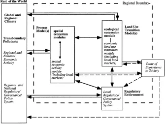
The overall model consists of interrelated ecological and economic submodels that employ a landscape perspective, for this perspective captures the spatial and temporal distributions of the services and functions of the natural system and human-related phenomena such as surrounding land-use patterns and population distri-butions (Bockstael and others 1995). Configuration and reconfiguration of the landscape occurs as a result of ecological and economic factors, and these factors are closely intertwined.
The ecological part of the model is based on the Patuxent Landscape Model (PLM), one of a series of landscape-level spatial simulation models as discussed above (Costanza and others 1995). The PLM is capable of simulating the succession of complex ecological systems using a landscape perspective. Economic submodels are being developed to reflect human behavior and eco-nomic influences. The effects of human intervention result directly from the conversion of land from one use to another (e.g., wetlands conversion, residential devel-opment, power plant siting) or from changes in the practices that take place within specific land uses (e.g., adoption of agricultural best management practices, intensification of congestion and automobile emissions, change in urban water and sewer use, and storm runoff).
Economic submodels will characterize land use and agricultural decisions and capture the effects on these
decisions of institutional influences such as environmen-tal, zoning, transportation, and agricultural policies. The integration of the two models provides a frame-work for regulatory analysis in the context of risk assessment, nonpoint source pollution control, wet-lands mitigation/restoration, etc. Figure 3 shows the relationship of the various model components.
The integrated model will allow stakeholders to evaluate the indirect effects over long time horizons of current policy options. These effects are almost always ignored in partial analyses, although they may be very significant and may reverse many long-held assump-tions and policy predicassump-tions. It will also allow us to directly address the functional value of ecosystem ser-vices by looking at the long-term, spatial, and dynamic linkages between ecosystems and economic systems.
Conclusions
The complexities that surround environmental invest-ments and problems require that nonlinearities and spatial and temporal lags be reflected in models used for decision support. Dynamic modeling is designed to address these system features. It also lends itself as a method to scope environmental problems and build consensus and has been used in an array of case studies ranging from industrial systems to ecosystems to linked ecological–economic systems.
In each case study described above, the three-stage modeling process enabled us to provide a set of detailed
conclusions regarding the management of the respec-tive system. These conclusions were built on models that embodied the input and expert judgment of a broad range of stakeholders. The modeling process also of-fered unique insight into our ability to anticipate a system’s dynamics in light of nonlinearities and of spatial and temporal lags. Our ability to anticipate those dynamics on the basis of available data and knowledge and to develop consensus about those dynamics is an essential prerequisite for the successful management of complex ecological-economic systems. We anticipate that future modeling efforts will increasingly make use of the software tools and the three-step modeling process with stakeholder involvement described in this paper.
Acknowledgments
An earlier version of this paper was presented at the inaugural conference of the European Chapter of the International Society for Ecological Economics, Univer-site´ de Versailles, Paris, France, 23–25 May 1996. Carl Folke, Marjan van den Belt, and Cutler Cleveland provided helpful comments on earlier drafts. The Pew Charitable Trusts and the Beijer International Institute for Ecological Economics provided support during manuscript preparation. Additional support was pro-vided by Roy F. Weston, Inc.
Literature Cited
Allen, P. 1988. Evolution, innovation and econopmics. In G. Dosi, C. Freeman, R. Nelson, G. Silvergerg, and L. Soete (eds.), Technical change and economic theory. Pinter, London.
Bahr, L. M., R. Costanza, J. W. Day, Jr., S. E. Bayley, C. Neill, S. G. Leibowitz, and J. Fruci. 1983. Ecological characteriza-tion of the Mississippi Deltaic Plain Region: a narrative with management recommendations. US Fish and Wildlife Ser-vice, Division of Biological Services, Washington, DC. FWS/ OBS-82/69, 189 pp.
Bockstael, N., R. Costanza, I. Strand, W. Boynton, K. Bell, and L. Wainger. 1995. Ecological economic modeling and valua-tion of ecosystems. Ecological Economics 14:143–159.
Bond, P., and P. Goldblatt. 1984. Plants of the Cape Flora.
Journal of South African Botany Suppl. 13:1–455.
Checkland, P. 1989. Soft systems methodology. In J. Rosenhead (ed.), Rational analysis for a problematic world. John Wiley & Sons, Chichester, England.
Cleveland, C. J., C. Neill, and J. W. Day, Jr. 1981. The impact of artificial canals on land loss in the Barataria Basin, Louisi-ana. Pages 425–434 In W. J. Mitsch, R. W. Bosserman, and J. M. Klopatek (eds.), Energy and ecological modeling. Elsevier, Amsterdam.
Costanza, R. 1987. Simulation modeling on the Macintosh using STELLA. BioScience 37:129–132.
Costanza, R., and J. Greer. 1995. The Chesapeake Bay and its watershed: A model for sustainable ecosystem management? Pages 169–213 in L. H. Gunderson, C. S. Holling and S. Light (eds.), Barriers and bridges to the renewal of ecosys-tems and institutions. Columbia University Press, New York, 593 pp.
Costanza, R., and T. Maxwell. 1993. Resolution and predictabil-ity: An approach to the scaling problem. Landscape Ecology 9:47–57.
Costanza, R., and F. H. Sklar. 1985. Articulation, accuracy, and effectiveness of mathematical models: A review of freshwater wetland applications. Ecological Modeling 27:45–68.
Costanza, R., C. Neill, S. G. Leibowitz, J. R. Fruci, L. M. Bahr, Jr., and J. W. Day, Jr. 1983. Ecological models of the Mississippi deltaic plain region: Data collection and presen-tation. US Fish and Wildlife Service, Division of Biological Services, Washington, DC. FWS/OBS-82/68, 340 pp. Costanza, R., F. H. Sklar, M. L. White, and J. W. Day, Jr. 1988. A
dynamic spatial simulation model of land loss and marsh succession in coastal Louisiana. Pages 99–114 in W. J. Mitsch, M. Straskraba, and S. E. Jørgensen (eds.), Wetland modelling. Elsevier, Amsterdam.
Costanza, R., F. H. Sklar, and M. L. White. 1990. Modeling coastal landscape dynamics. BioScience 40:91–107.
Costanza, R., H. C. Fitz, T. Maxwell, A. Voinov, H. Voinov, and L. A. Wainger. 1995. Patuxent landscape model: Sensitivity analysis and nutrient management scenarios. Interim Re-port for US EPA Cooperative Agreement CR 821925010. University of Maryland Institute for Ecological Economics, Center for Environmental and Estuarine Studies, University of Maryland, Box 38, Solomons, Maryland 20688-0038. Cowling, R. M. (ed.). 1992. The ecology of fynbos. Nutrients,
fire and diversity. Oxford University Press, Cape Town. Cowling, R. M., P. M. Holmes, and A. G. Rebelo. 1992. Plant
diversity and endemism. Pages 62–112 in The ecology of fynbos. Nutrients, fire and diversity. R. M. Cowling (ed.), Oxford University Press, Cape Town.
Craig, N. J., R. E. Turner, and J. W. Day, Jr. 1979. Land loss in coastal Louisiana (U.S.A.). Environmental Management 3:133– 144.
Deegan, L. A., H. M. Kennedy, and C. Neill. 1984. Natural factors and human modifications contributing to marshloss in Louisiana’s Mississippi River deltaic plain. Environmental
Management 8:519–528.
Gagliano, S. M., K. J. Meyer-Arendt, and K. M. Wicker. 1981. Land loss in the Mississippi River Deltaic Plain. Transactions
of the Gulf Coast Association of Geological Societies 31:285–300.
Granger, C. W. J. 1969. Investigating causal relations by econometric models and cross-spectral methods.
Economet-rica 37:424–438.
Granger, C. W. J. 1993. What are we learning about the long run? Economic Journal 103:307–317.
Groffman, P. M., and G. E. Likens (eds.). 1994. Integrated regional models: Interactions between humans and their environment. Chapman and Hall, New York, 157 pp. Gunderson, L., C. S. Holling, and S. Light (eds.). 1995.
Hannon, B., and M. Ruth. 1994. Dynamic modeling. Springer-Verlag, New York.
Hannon, B., and M. Ruth. 1997. Modeling dynamic biological systems. Springer-Verlag, New York.
Higgins, S. I., Turpie, J. K., Costanza, R., Cowling, R. M., Le Maitre, D. C., Marais, C., and Midgley, G. F. 1996. An ecological economic simulation model of mountain fynbos ecosystems: Dynamics, valuation and management.
Ecologi-cal Economics (submitted).
Hobbs, R. J., D. M. Richardson, and G. W. Davis. 1995. Mediterranean-type ecosystems: opportunities and con-straints for studying the function of biodiversity. Pages 1–42
in G. W. Davis and D. M. Richardson (eds.),
Mediterranean-type ecosystems. The function of biodiversity. Springer, Berlin.
Hogarth, R. 1987. Judgment and choice. John Wiley & Sons, Chichester, England.
Holling, C. S. 1964. The analysis of complex population processes. The Canadian Entomologist 96:335–347.
Holling, C. S. 1966. The functional response of invertebrate predators to prey density. Memoirs of the Entomological Society
of Canada No. 48.
Holling, C. S. (ed.). 1978. Adaptive environmental assessment and management. Wiley, London.
Kahnemann, D., and A. Tversky. 1974. Judgment under uncertainty. Science 185:1124–1131.
Kahnemann, D., P. Slovic, and A. Tversky. 1982. Judgment under uncertainty: Heuristics and biasis. Cambridge Univer-sity Press, Cambridge.
Kraemer, K. L., and J. L. King. 1988. Computer-based systems for cooperative work and group decisionmaking. ACM
Computing Surveys 20:115–146.
Leamer, E. 1983. Let’s take the ‘con’ out of econometrics.
American Economic Review 73:31–43.
Lee, K. 1993. Compass and the gyroscope. Island Press, Washington DC.
Leibowitz, S. 1989. The pattern and process of land loss in coastal Louisiana: A landscape ecological analysis. PhD dissertation. Louisiana State University, Baton Rouge, Loui-siana.
Leontief, W. 1982. Academic economics. Science 217:104– 107. Levins, R. 1966. The strategy of model building in population
biology. American Scientist 54:421–431.
Lyneis, J. M. 1980. Corporate planning and policy design: A system dynamics approach. Pugh-Roberts Associates, Cam-bridge, Massachusetts.
Morecroft, J. D. W. 1994. Executive knowledge, models, and learning. Pages 3–28 in J. D. W. Morecroft and J. D. Sterman (eds.), Modeling for learning organizations. Productivity Press, Portland, Oregon.
Morecroft, J. D. W., and K. A. J. M. van der Heijden. 1994. Modeling the oil producers: Capturing oil industry knowl-edge in a behavioral simulation model. Pages 147–174 in J. D. W. Morecroft and J. D. Sterman (eds.), Modeling for learning organizations. Productivity Press, Portland, Or-egon.
Morecroft, J. D. W., D. C. Lane, and P. S. Viita. 1991. Modelling growth strategy in a biotechnology startup firm. System
Dynamics Review 7:93–116.
Myers, N. 1990. The biodiversity challenge: expanded hot-spots analysis. The Environmentalist 10:243–255.
Oster, G. 1996. Madonna, http://nature.berkeley.edu/, gos-ter/madonna.html.
Peterson, S. 1994. Software for model building and simulation: An illustration of design philosophy. Pages 291–300 in J. D. W. Morecroft and J. D. Sterman (eds.), Modeling for learning organizations. Productivity Press, Portland, Oregon. Phillips, L. D. 1990. Decision analysis for group decision
support. In C. Eden and J. Radford (eds.), Tackling strategic problems: The role of group decision support. Sage Publish-ers, London.
Rao, S. S. 1994. Welcome to open space. Training April: 52–55. Rawls, J. 1971. A theory of justice. Oxford University Press,
Oxford England.
Rawls, J. 1987. The idea of an overlapping consensus. Oxford
Journal of Legal Studies 7:1–25.
Richmond, B., and S. Peterson. 1994. STELLA II documenta-tion. High Performance Systems, Inc., Hanover, New Hamp-shire.
Roberts, E. B. 1978. Managerial applications of system dynam-ics. Productivity Press, Portland, Oregon.
Roberts, H. H., R. D. Adams, and R. H. Cunningham. 1980. Evolution of the sand-dominated subaerial phase, Atchafa-laya delta, Louisiana. American Association of Petroleum
Geolo-gists Bulletin 64:264–279.
Robinson, J. B. 1991. Modelling the interactions between human and natural systems. International Social Science
Jour-nal 130:629–647.
Robinson, J. B. 1993. Of maps and territories: The use and abuse of socio-economic modelling in support of decision-making. Technological Forecast and Social Change (in press). Rosenhead, J. (ed.). 1989. Rational analysis of a problematic
world. John Wiley & Sons, Chichester, England.
Ross, M. 1987. Industrial energy conservation and the steel industry of the United States, Energy 12:1135–1152. Ruth, M. 1993. Integrating economics, ecology and
thermody-namics, Kluwer Academic Publishers, Dordrecht, The Neth-erlands.
Ruth, M. 1995. Technology change in US iron and steel production: Implications for material and energy use, and CO2emissions. Resources Policy 21:199–214.
Ruth, M. 1997. Energy use and CO2emissions in a
dematerial-izing economy: Examples from five US metals sectors. Mimeograph. Center for Energy and Environmental Stud-ies, Boston University, Boston, Massachusetts.
Ruth, M., and C. J. Cleveland. 1996. Modeling the dynamics of resource depletion, substitution, recycling and technical change in extractive industries. Pages 301–324 in R. Cos-tanza, O. Segura, and J. Martinez-Alier (eds.), Getting down to earth: Practical applications of ecological economics. Island Press, Washington, DC.
Ruth, M., and B. Hannon. 1997. Modeling dynamic economic systems. Springer-Verlag, New York.
Ruth, M., and T. Harrington. 1997. Dynamic of material and energy use in US pulp and paper manufacturing. Journal of
Industrial Ecology (in press).
Scaife, W. W., R. E. Turner, and R. Costanza. 1983. Coastal Louisiana recent land loss and canal impacts. Environmental
Management 7:433–442.
Senge, P. M. 1990. The fifth discipline. Doubleday, New York. Senge, P. M., and J. D. Sterman. 1994. Systems thinking and
organizational learning: Acting locally and thinking globally in the organization of the future. Pages 195–216 in J. D. W. Morecroft and J. D. Sterman (eds.), Modeling for learning organizations. Productivity Press, Portland, Oregon. Simon, H. A. 1956. Administrative behavior. Wiley, New York. Simon, H. A. 1979. Rational decision-making in business
organizations. American Economic Review 69:493–513. Sklar, F. H., R. Costanza, and J. W. Day, Jr. 1985. Dynamic
spatial simulation modeling of coastal wetland habitat succes-sion. Ecological Modelling 29:261–281.
Sklar, F. H., M. L. White, and R. Costanza. 1989. The coastal ecological landscape spatial simulation (CELSS) model: Structure and results for the Atchafalaya/Terrebonne study area. US Fish and Wildlife Service, Division of Biological Services; Washington, DC.
Sparrow, F. T. 1983. Energy and material flows in the iron and steel industry. Argonne National Laboratory, Argonne, Illinois. ANL/CNSV-41.
Van Heerden, I. L., and H. H. Roberts. 1980a. The Atchafalaya delta—Louisiana’s new prograding coast. Transactions, Gulf Coast Association of Geological Societies 30:497–506. Van Heerden, I. L., and H. H. Roberts. 1980b. The Atchafalaya
delta—rapid progradation along a traditionally retreating
coast (south central Louisiana). Zeitschriftfuer Geomorphologie
N.F. 34:188–201.
Vennix, J. A. M., and J. W. Gubbels. 1994. Knowledge elicita-tion in conceptual model building: A case study in modeling a regional Dutch health care system. Pages 121–146 in J. D. W. Morecroft and J. D. Sterman (eds.), Modeling for learning organizations. Productivity Press, Portland, Or-egon.
Walters, C. J. 1986. Adaptive management of renewable resources. McGraw-Hill, New York.
Weisbord, M. (ed.). 1992. Discovering common ground. Ber-rett-Koehler, San Francisco, 442 pp.
Weisbord, M., and S. Janoff. 1995. Future search: An action guide to finding common ground in organizations and communities. Berrett-Koehler, San Francisco.
WCED. 1987. Our Common Future: Report of the World Commission on Environment and Development. Oxford University Press, Oxford.
Westenholme, E. F. 1990. System inquiry: A system dynamics approach. John Wiley & Sons, Chichester, England.
Westenholme, E. F. 1994. A systematic approach to model creation. Pages 175–194 in J. D. W. Morecroft and J. D. Sterman (eds.). Modeling for learning organizations. Produc-tivity Press, Portland, Oregon.
Weston, R. F., and M. Ruth. 1997. A dynamic hierarchical approach to understanding and managing natural eco-nomic systems. Ecological Ecoeco-nomics 21:1–17.