Parameter Identification of a Brushless Resolver Using Charge Response of Stator Current

Parameter Identification of a Brushless Resolver Using

Charge Response of Stator Current

D. Arab-Khaburi*, F. Tootoonchian* and Z. Nasiri-Gheidari**

Abstract: Because of temperature independence, high resolution and noiseless outputs, brushless resolvers are widely used in high precision control systems. In this paper, at first dynamic performance characteristics of brushless resolver, considering parameters identification are presented. Then a mathematical model based on d-q axis theory is given. This model can be used for studying the dynamic behavior of the resolver and steady state model is obtained by using dynamic model. The main object of this paper is to present an approach to identify electrical and mechanical parameters of a brushless resolver based on DC charge excitation and weight, pulley and belt method, respectively. Finally, the model of resolver based on the obtained parameters is simulated. Experimental results approve the validity of proposed method.

Keywords: Brushless Resolver, Dynamic Performance, Electrical and Mechanical Parameter Identification, Steady State Behavior.

1 Introduction1

In High-performance brushless motor systems like inverter-driven permanent-magnet synchronous motor (PMSM), absolute rotor-position with high accuracy and resolution, is necessary for realizing vector control. Among various existing position sensors [1, 2], those which can provide absolute position are resolvers and optical absolute encoders. Both of them provide reliable and precise rotor position signals. So comparing with optical absolute encoders, resolvers are more mechanically reliable, and easy to be integrated with motor systems [3]. Traditional resolvers have brushes and slip-rings; but in brushless resolvers, brushes are replaced by a rotary transformer [4].

The simplified dynamic equations of resolvers have been presented in [5], in which the effects of stator current and eccentricity have been neglected and the steady state behavior of resolver has not been presented too. Ref. [6] describes a magnetic field analysis method to determine an optimal magnetic design which eliminates harmonics, using 2-D FEM (two-dimensional finite element method). But, it’s time consuming process. Also authors mentioned that their method is not accurate and practical enough [6].

Iranian Journal of Electrical & Electronic Engineering, 2007. * Davood Arab-Kahburi and Farid Tootoonchian are with the Department of Electrical Engineering, Iran University of Science and Technology, Tehran, Iran.

E-mail: [email protected] and [email protected]

** Zahra Nasiri-Gheidari is with the Department of Electrical Engineering, Sharif University of Technology, Tehran, Iran.

E-mail: [email protected]

On the other hand, many papers have reported on the accuracy of resolver to digital converters [7-11] and there are some papers that present parameters identification methods for rotary transformers [12]; but parameter estimation of brushless resolver has not been discussed.

The purpose of this paper is to present a mathematical model to predict the behavior of the brushless resolver and its equivalent circuit which is similar to induction motor's steady state equivalent circuit. Therefore the methods used to identify induction motor’s parameters, can be used with brushless resolver. In literatures there are many methods for determination of induction motor parameters [13-19]. Some of these methods are based on genetic algorithms [13, 14] or neural networks [15, 16]. Other works are performed to improve the accuracy [17, 18] and there are some works to reduce time of tests [19]. Each of these methods has its advantages and disadvantages. This paper presents a DC-Pulse method based on a simple configuration, which increase estimated parameters accuracy and reduce time of test. In this method, brushless resolver’s parameters are determined by analyzing the stator currents response to the DC-Pulse voltage, applied to the stator windings. An exponential curve is fitted to the stator current response in DC charge condition. Coefficients and time constants of these fitted curves can be determined. Then brushless resolver parameters will be calculated according to the related equations. Of course DC charge method is only used for electrical parameters identification but mechanical parameters (moment of inertia) must be measured using other methods.

Finally simulation results are compared with experimental ones and good agreement between them approves the parameters accuracy.

2 Resolver Model and Current Equation

The following assumptions are considered in the analysis:

a) Stator is assumed to have a sinusoidally distributed polyphase windings.

b) Rotor has a winding with sinusoidal supply.

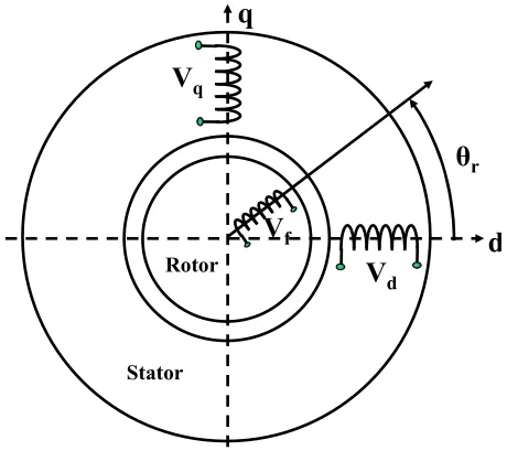
Figure 1 shows the model of resolver. Each stator winding flux consists of leakage flux and main flux, the latter flux links the rotor.

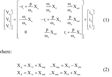
The stator variables are transformed to the rotor reference frame which eliminates the time-varying inductances in the voltage equations. Park’s equations are obtained by setting the speed of the stator frame equal to the rotor speed. So, the voltage-current equations are as follows:

r r

s q d md

b b b

q q

r

d q s d md d

b b b

r r

md r rr

b b

p

r X X X

V i

p p

V X r X X i

V i

p p

0 X r X

_{− +} ω ω 

 _{ω ω ω} 

 

   

 ω 

 _{= − − + ×} 

 

  _{ω ω ω}  

            +   ω ω     (1) where: ms 0 md md s d ms 0 mq mq s q X X X , X X X X X X , X X X + = + = − = + = (2)

And p is d/dt, Vq, Vd are the q-d axis stator voltages, Vr

is the excitation signal of the resolver (V_r =v cos(_r′ ω + ψ_ft )), iq, id are the d, q axis stator

currents, ir is the rotor current, rs is the resistance of

stator circuit; Xℓs, Xms are, respectively, the leakage and

magnetizing reactance of the stator winding; rr, Xrr are

the resistance and reactance of rotor circuit, Xmd , Xmq

are d-q axis mutual inductance between rotor and stator circuits, ωb is base angular frequency and ωr is the rotor

angular frequency.

The electromagnetic torque developed in the resolver is given by:

(

d q q d

)

b

em i i

2 P

T ψ −ψ

ω

= ₍₃₎

And the mechanical equation of resolver in per unit can be written as:

( )

( )

( )

dt d H 2 pu T pu T pu T b r damp mech em       ω ω = − + (4)

where H is the inertia constant expressed in second, Tmech is Load torque and Tdamp is fractional torque.

For steady state conditions the electrical angular velocity of the rotor is constant and equal to ωe,

whereupon the electrical angular velocity of the synchronously rotating reference frame. In this mode of operation the rotor windings do not experience a change of flux linkages [20]. Thus, with ωr set equal to ωe and

the time rate of change of all flux linkages neglected, the steady state versions of (1) become:

r r r e r q q b e d s d e d r md b e d d b e q s q e q I r V V I x I r V V I x I x I r V V ′ ′ − = ′ = ′ ω ω + − = = ′ ω ω + ω ω − − = = (5)

Here the ωe to ωb ratio is again included to

accommodate analysis when the operation frequency is other than rated.

In the synchronously rotating reference frame and using uppercase letters to denote the constant steady state variables:

e ds e qs as F jF

F ~

2 = − (6)

where F is each electrical variable (voltage, current, flux linkage), Fas

~

is a phasor which represents a sinusoidal quantity; e

qs

F and e ds

F are real quantities representing the constant steady state variables of the synchronously rotating reference frame. Hence

e d e q as V jV

V~

2 = − (7)

Substituting (5) into (7) yields:

(

)

      ′ ω ω + − ω ω − +       ω ω + − = r md b e d q d b e d q b e s as I X I X X 2 1 I ~ X r V~ 2 (8)

For symmetrical resolver, Xd =Xq and ωe= ωb. So (8) can

be writing as:

(

)

r m a a as s s as I X 2 1 E~ E~ I ~ jX r V~ ′ = + + − = (9) where m s

s X X

X = + (10)

q

d

θ

_r

V

_d

V

_q

V

_f Rotor Stator

Fig. 1 Resolver model.

Considering above equations the steady state equivalent circuit of resolver is shown in Fig. 2.

It is to be noticed that stator and rotor phase number in the induction motor can be assumed equal, but resolver is similar to a synchronous generator with single phase sinusoid excitation. For using DC charge method for parameter identification in resolver, the rotor position must be at the angular position that is right as one phase and vertical versus other phase winding, and the latter phase winding, should be shorted. Fig. 3 shows the resolver equivalent circuit at this position which is similar to equivalent circuit of induction motor.

If the stator winding of the resolver is excited by a DC step voltage, the stator current transfer function based on the circuit model of Fig. 3, can be obtained as follows [21]: ) T T ( s ) T T ( s 1 sT 1 . s 1 . r V . 2 1 ) s ( I s r 2 s r r s

s _{+ + + σ}

+

= (11)

Applying inverse Laplace transformation equation (11), stator current in time domain can be written as:

) e A e A ( A ) t (

i 1 T2

t 2 T t 1 0 s − − + = (12) where: lr m r r r

r , L' L L'

' r

' L

T = = + ₍₁₃₎

ls m s s

s

s , L L L

r L

T = = + ₍₁₄₎

s r m 2 L '. L L 1− = σ ₍₁₅₎ s s 0 r V . 2 1

A = ₍₁₆₎

1 2 2 1 r AT AT

T = − ₍₁₇₎

s

r

jx

_s

m

x

r ' r 2 r ' jX 2 as

V

~

++++

−−−−

++++

−−−−

r

V

′

Ia I′r/ 2

Fig. 2 Steady state equivalent circuits of the resolver.

Is rs⇒Rs Lls

m

L

r f R

r′ ⇒ ′

lr lf L

L' ⇒ '

s

V

~

++++

−−−−

++++

−−−−

0 = ′ r V

Fig. 3 Equivalent circuit of resolver with shorted rotor.

1 s r 2 T T T

T = + − ₍₁₈₎

2 s r 1 T T T

T =σ ₍₁₉₎

Now, if coefficients A1, A2 and time constants T1, T2 are

known; electrical parameters of the resolver can be identified.

3 Experimental Test Setup

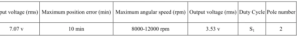
Figure 4 shows the manufactured resolver and experimental setup of it. The experimental resolver was a pancake resolver with the specifications, which presented in Table 1.

The DC voltage source of this setup is chosen to provide rated current of resolver. When switch S is closed, stator current (Is) will be sensed by Hall-Effect current sensor

and its output voltage is delivered to the PC via an A/D cart or monitored on digital oscilloscope.

Experimental recorded data of current curve is shown in Fig. 5 and this curve is fitted by exponential equation of (12).

(a)

Stator of Resolver s

R

L

ls

L

'

lr

R

'

r

N1 N2

Rotor of Resolver

A

2

D

Digital Oscilloscope

DC

V

Hall Effect

Sensor

L

_m

S

(b)

(c)

Fig. 4 (a) Schematics of test resolver, (b) schematic of test setup, (c) Experimental setups of the test resolver for DC charge test.

Table 1 Spesifications of tested resolver.

Pole number Duty Cycle

Output voltage (rms) Maximum angular speed (rpm)

Maximum position error (min) Input voltage (rms)

2 S1

3.53 v 8000-12000 rpm

10 min 7.07 v

Therefore current equation's coefficients and time constants can be obtained.

Finally using equations (13-19), brushless resolver parameters are calculated. Estimated parameters are presented in Table 2.

After electrical parameter identification, mechanical parameter (momentum of inertia) should be estimated.

The momentum of inertia is most important mechanical parameter of resolver. Many different methods are presented for calculation of the momentum of inertia in [22]. Some of them measured J after disconnecting rotor from resolver, such as Pendulum method and tensional vibration. But there is other mechanical method that can measure rotor inertia, without disconnecting rotor,

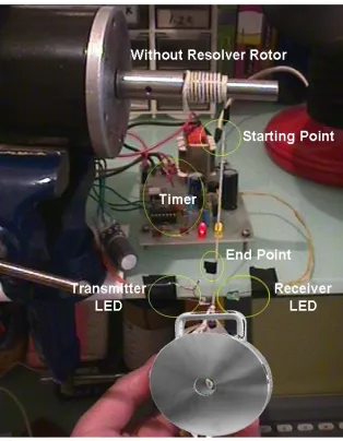
by using weight, pulley and belt. The pulley is made of lightweight polymer. Of course, in this method we require a lightweight belt, some weights and two optical keys, which used for accurate time calculation, in both ends. Fig. 6 shows the experimental setup of resolver. The momentum of inertia is calculated with and without DC coupled motor.

In this method, weight acceleration is:

2 2 1

2 1

2 1 2 1

) t t (

) x x ( 4 ) x x ( 2 a

− − +

= (20)

where a is linear acceleration of weight, (t1-t2) is the

time required for displacement from x1 to x2.

In (20), we supposed that acceleration is constant at t2-t1

and weights are heavy enough that can overcome to friction. By ignoring of bearing and brush friction:

p 2

J r . W ) g 1 ( ) a 1 (

J −

   

 

−

= ₍₂₁₎

Table 2 Estimated parameters based on discharge method.

rs [Ω] 40

Lls [H] 0.2×10

-3

Lm [H] 2.089×10-3

r'r [Ω] 19

L'lr [H] 0.2×10-3

Fig. 5 Current response to the DC step voltage (Experimental test).

Fig. 6 Schematic of pulley, weight and band free acceleration.

Now by applying bearing and brush frictions: F r ) g / a . W W ( r a ). J J ( _P − − = + (22)

where W is Wight of weights, g is gravitation acceleration, r is pulley radius, Jp is pulley momentum

of inertia and F is friction force. Since, friction force is constant up to nominal speed [22], by subtracting two set of data, the momentum of inertia is calculated as:

{

}

) a a ( r g / ) a w a w ( w w J 1 2 2 1 1 2 2 1 2 − − − − = ₍₂₃₎

That is calculated for tested resolver:

] [kg.m 4 -10 1.24

J_{= ×} 2

(24)

4 Method Validation

4.1 Simulation

The state equations on the rotating dq0 reference frame are introduced. MATLAB/Simulink software is used for simulation purposes.

Input, out put and state variables are:

t r mech r r ds qs ] [ or OutputVect ] T , V [ r InputVecto ] , , [ bles StateVaria θ ∆ = ∆ ′ = ψ′ ψ ψ = (25)

Equation (1) shows the voltage-current relations. However, it is more convenient to use flux-linkages as the state variables [23]. Therefore, the currents versus flux-linkages are calculated from (5).

Considering linkages as state variables, flux-linkage equations are obtained as follow:

(

)

dt

X r V d b r q mq s s q b

q

∫



     ψ ω ω − ψ + ψ − + ω = ψ (26)

(

)

∫

_     ψ ω ω + ψ + ψ − + ω = ψ dt X r V q b r d md s s d b d (27)

(

)

dt

X r

V md r

r r r b

r

∫



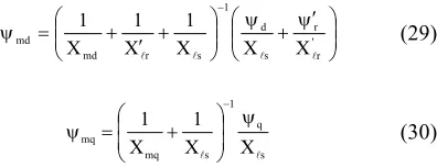
     ψ′ − ψ ′ ′ + ′ ω = ψ′ (28) where       ψ′ + ψ       + ′ + = ψ − ' r r s d 1 s r md md X X X 1 X 1 X 1 (29) s q 1 s mq mq X X 1 X 1 ψ         + = ψ − (30)

Now the output angular position, stator and rotor current can be calculated as:

( ) ( )

t t

( )

t

( ) (

t

)

dt _r

( )

0 _e

( )

0

t

0 e r e

r −θ = ω −ω +θ −θ

θ = δ =

θ

∫

₍₃₁₎

s mq q q x i ψ − ψ = ₍₃₂₎ s md d d x i ψ − ψ = ₍₃₃₎ r md r r x i ′ ψ − ψ′ = ′ ₍₃₄₎

In symmetrical resolver d-q axis impedances are equal. Therefore in the above equations Xd is equal to Xq. It is

considerable that the proposed model is able to describe eccentric resolver by setting unequal amount of Xd and

Xq (Xd ≠ Xq). Performance prediction of eccentric

resolver will be studied in another paper.

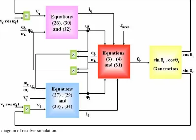
Figure 7 shows the simulation block diagram of resolver.

4.2 Results andDiscussions

Figure 8 shows the manufactured resolver and experimental setup of it. The resolver was tested using the 100 watt, 12000 r.p.m. DC motor.

It is to be noted, simulation and measured result can be compared in two categories:

(a) Loading test of resolver, because it is similar to a synchronous generator with sinusoid excitation.

(b) Comparing of position data since the resolver is a position sensor.

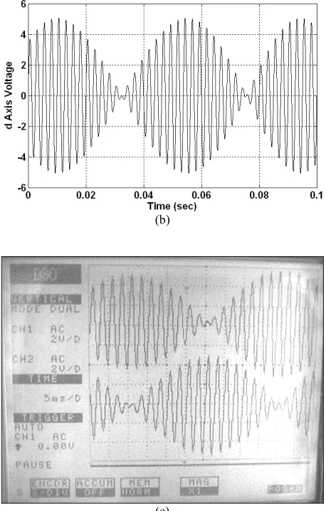
Figure 9 shows the test and computed d-q voltages of resolver with 4000 (Hz) excitation and the nominal output current (10 mA).

Fig. 7 Block diagram of resolver simulation.

Manufactured Resolver

DC Motor

(a) (b)

Fig. 8 (a) Schematics of test resolver, (b) Experimental setups of the test resolver.

(a) (b)

(c)

Fig. 9 Output voltage of resolver versus time with 4000 Hz excitation and 10 mA output current (a) simulated q-axis voltage (b) simulated d-axis voltage and (c) measured q-d axis voltage.

It has been shown that the amplitude of the measured voltage is slightly larger than simulated one and the maximum amplitude error is about +5.89%. This error maybe comes from capacitive effect of winding in high frequency operation which is ignored in our simulation. So the simulation and experiments has been repeated with the same current and lower excitation frequency such as one tenths of nominal frequency (0.1×fn=400

Hz). Figure 10 shows the results of recent condition. Maximum error decreases to -1.78%. This error reduction confirms the capacitive effect.

In practice, resolvers are loaded by RDCs (Resolver to Digital Converters). The input impedance of RDC is very high. So resolver’s stator currents are in the order of micro amperes (According to AD2S80 datasheet). Therefore the capacitive effect can be neglected at practice.

Figure 11 shows test’s results in the nominal frequency (4 kHz) and 60 µA output current (5×nominal current of RDC-AD2S80). It can be seen good agreement between calculated and experimental results (maximum error is about +1.19%).

(a)

(b)

(c)

Fig. 10 Output voltage of resolver versus time with 400 Hz excitation and 10 mA output current (a) simulated q-axis voltage (b) simulated d-axis voltage and (c) measured q-d axis voltage.

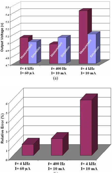
Table 3 and Fig. 12 show the comparison of the simulation and exprimental results that validate the resolver model and parameter estimation method. It is obvious that resolver is a position sensor, so comparison of sensor output (position) is important. For practical test we used from a high precision mechanical position sensor (tycope1) that connected to VF5-HP20 CNC (Computer Numeric Control) Machine. The resolver output is obtained from arctangent of output voltages ratio.

Figure 13 shows the position outputs from simulation, resolver and high precision mechanical position sensor (tycope). Comparison of these results shows that the maximum position error of resolver is ±3 Arcmin. Therefore these results validate the accuracy of proposed parameter estimation method. Since proposed setup doesn’t need any extra equipments and it has simple test configuration, this method is not only accurate but also simple and fast.

1_{The Tycope is a mechanical gearbox with high rotary reduction ratio} (1:n, 500<n<3000). It can divide rotary position into small parts.

(a)

(b)

(c)

Fig. 11 Output voltage of resolver versus time with 4000 Hz excitation and 60 µA output current (a) simulated q-axis voltage (b) simulated d-axis voltage and (c) measured q-d axis voltage.

Table 3 Comparision of calculated and measured resuls.

Error (%) Output voltage

(measured) Output voltage

(simulated) Frequency

(Hz) Output

current (mA)

+5.89 5.43

5.11 4000

10

-1.78 4.97

5.06 400

10

+1.19 5.06

5 4000

0.060

(a)

(b)

Fig. 12 Comparisons of calculated and measured results of resolver as electrical machinery (a) output voltage (volt) (b) relative error (%).

Simulation

Resolver Output

High precision position sensor output

Fig. 13 Comparison of calculated angular position with

resolver output and tycope output.

5 Conclusions

In this paper a new dynamic and steady state analysis of brushless resolver has been presented and a new approach based on DC step voltage excitation is presented and applied to brushless resolver stator windings. Stator current is measured and current curve is drawn. Using equivalent circuit of resolver at steady state, the current equation is obtained; the curve is fitted to an exponential current curve, to determine

coefficients and time constants. By using known equations, resolver parameters are estimated. The experimental test for a definite load validates obtained results.

Advantages of this method are:

• Simplicity of configuration

• Accuracy of the results

• Reduction of the time consuming.

Furthermore, steady state equivalent circuits of a brushless resolver are presented as first time.

References

[1] Harnefors L. and Nee H. P., “A General Algorithm for Speed and position Estimation of AC Motors,” IEEE Trans. Industrial Electronics, Vol. 47(1), pp. 77-83, Feb. 2000.

[2] Caricchi F., Capponi F. G., Crescimbini F., and Solero L., “Sinusoidal brushless drive with low-cost linear Hall Effect Position sensors,” IEEE PESC 2001, Vol.2, pp. 17-21, 2001.

[3] Hanselmar D. C, Thibodeau R. E. and Smith D. J., “Variable-reluctance Resolver Design Guidelines,” IEEE IECON, New York, pp. 203-208, 1989.

[4] Sun L. Z., Zou J. B. and Lu Y. P., “New Variable-reluctance resolver for Rotor-position sensing,” IEEE conference, pp. 5-8, 2004. [5] Jiuqing W., Xingshan Li and Hong G., “The

Analysis and Design of High-speed Brushless Resolver plus R/D Converter Shaft-angle Measurement system,” IEEE conference, pp. 289-292, 2000.

[6] Masaki K., Kitazawa K., Mimura H., Nirei M., Tsuchimichi K., Wakiwaka H. and Yamada H., “Magnetic field analysis of a resolver with a skewed and eccentric rotor,” Elsevier trans. Sensors and Actuators, Vol. 81, pp. 297-300, 2000.

[7] Masaki K., Kitazawa K., Mimura H., Tsuchimichi K., Wakiwaka H., Yamada H., “Consideration on the angular error due to the shaft eccentricity and the compensation effect by short-circuit winding on a resolver,” J. Magn. Soc. Jpn. 22, pp. 701– 704, 1998.

[8] Munay B. A., Li. W. D., “A Digial Tracking R/D Converter with Hardware Error Calculation Using a TMS320C14,” Fifth European Conference on Power Electronics and Applications, pp. 472-477, 13-16, Sep. 1993.

[9] Yim Ch., Ha I., KO M. S., “A Resolver-to-Digital Convertion Method for Fast Tracking,” IEEE Transactions on Industrial Electronics, Vol. 39, Issue 5, pp. 369-378, Oct 1992.

[10] Hanselman D. C., “Techniques for Improving Resolver-to-Digital Conversion Accuracy,” IEEE Trans. on Industrial Electronics, Vol. 38, No. 6, pp. 501-504, Dec. 1991.

[11] Axsys Company R&D Group, “Pancake Resolvers Handbook”, http://www. Axsys.com, received at 15 December 2006.

[12] Khaburi D. A., Tootoonchian F., “Design, Parameter Identification and Simulation of Single-Phase Rotary Transformer,” 15th Iranian Conference on Electrical Engineering, ICEE2007, May 15-17, 2007.

[13] Weatherford H. H, Brice C. W., “Estimation of Induction Motor Parameters by a Genetic Algorithm,” Pulp and Paper Industry Technical Conference 2003 annual, pp. 21-28, 16-20 June 2003.

[14] Phumiphak T., Chat-Uthai C., “Estimation of Induction Motor Parameters Based on Field Test Coupled with Genetic Algorithm,” Proc. of Power System Technology 2002, International Conference on Power Con. 2002, Vol. 2, pp. 1199-1203, 13-17 Oct. 2002.

[15] Martinez L. Z., Martinez A. Z., “Identification of Induction Machines Using Artificial Neural Networks,” Proc. of IEEE ISIE 97, Vol. 3, pp. 1259-1264, 7-11 July 1997.

[16] Kabache N., Chetate B., “Adaptive Nonlinear Control of Induction Motor Using Neural Networks,” Proc. of Physics and Control International Conference 2003, Vol. l, pp. 259-264, 20-22 Aug., 2003.

[17] Macek-Kaminska K., Wach P., “Estimation of the Parameters of Mathematical Models of Squirrel Cage Inductions Motors,” Proc. Of IEEE ISIE 96, Vol. 1, pp. 337-342, 17-20 June 1996.

[18] Noguchi T., Nakmahachalasint P., Watanakul N., “Precise Torque Control of Induction Motor with On-Line Parameter Identification in Consideration of Core Loss,” Proc. of Power Conversion Conference-Nagaoka 1997, Vol. 1, pp. 113-118, 3-6 Aug. 1997.

[19] Lesani H., Nasiri Gheidari Z., Tootoonchian F., “A Novel P.C. Base Electromotor’s Dynamometery,” 3rd International Conference on “Technical and Physical Problems in Power Engineering” (TPE-2006), Gazi University, Ankara, TURKEY, May 29-31, pp. 222-226, 2006.

[20] Krause P. C., Analysis of Electrical Machinery, McGraw-Hill series in electrical engineering. Power & energy, 1986.

[21] Ziary I., Vahedi A., “Identification of Single-Phase Induction Motor Parameters Using Average Charge Response of Stator Currents,” ICEE 2004, Vol. 1, pp.260-264, 2004.

[22] I-Hai Lin P., Messal E. E., “Design of a Real-Time Rotor Inertia Estimation System for Motors

with a Personal Computer,” IEEE

Instrumentation and Measurement Technology Conference, IEEE Catalog No. 91CH2940-5, pp. 292-296, 1991.

[23] Ong C., Dynamic Simulation of Electric Machinery Using Matlab/Simulink, Prentice Hall PTR. Upper Saddle River, New Jersey, 1998.

Davood Arab-khaburi was born in

1965. He has received B.Sc. in 1990 from Sharif University of Technology in Electronic Eng. and M.Sc. and Ph.D. from ENSEM INPEL, Nancy, France in 1994 and 1998 respectively. He also worked at UTC in Compien, France (1998-1999). Since 2000 he has been a faculty member of Iran University of Science and technology. His research interests are Power Electronic and Motor Control.

Farid Tootoonchian has received

his B.Sc. and M.Sc. degrees in Electrical Engineering from the Iran University of Science and Technology, Tehran, Iran in 2000 & 2007 respectively. He has done over 21 industrial projects including one national project about electrical machines over the years, and holds 5 patents. His research interest is design of small electromagnetic machines and sensors.

Zahra Nasiri-Gheidari has

received her B.Sc. degree in Electrical Engineering from the Iran University of Science and Technology, Tehran, Iran in 2004. And she received the Master degree in Electrical Power Engineering from the University of Tehran in Iran in 2006, graduating with First Class Honors in both of them. She is currently director of Electrical machinery Lab. in the Electrical Engineering Department of Sharif University of Technology, Tehran, Iran. Her research interests are design and modeling of electrical machines and drives.