http://dx.doi.org/10.4236/jilsa.2012.41007 Published Online February 2012 (http://www.SciRP.org/journal/jilsa)
An Improved Genetic Algorithm for Crew Pairing
Optimization
Bahadır Zeren, İbrahim Özkol
Faculty of Aeronautics and Astronautics, Istanbul Technical University, Istanbul, Turkey. Email: [email protected], [email protected]
Received July 23rd, 2011; revised December 27th, 2011; accepted January 6th, 2012
ABSTRACT
Crew pairing is a sequence of flights beginning and ending at the same crewbase. Crew pairing planning is one of the primary processes in airline crew scheduling; it is also the primary cost-determining phase in airline crew scheduling. Optimizing crew pairings in an airline timetable helps minimize operational crew costs and maximize crew utilization. There are numerous restrictions that must be considered and just as many regulations that must be satisfied in crew pairing generation. The most important regulations—and the ones that make crew pairing planning a highly constrained optimization problem—are the the limits of the flight and the duty periods. Keeping these restrictions and regulations in mind, the main goal of the optimization is the generation of low cost sets of valid crew pairings which cover all flights in the airline’s timetable. For this research study, We examined studies about crew pairing optimization and used these previously existing methods of crew pairing to develop a new solution of the crew pairing problem using genetic algo- rithms. As part of the study we created a new genetic operator—called perturbation operator. Unlike traditional genetic algorithm implementations, this new perturbation operator provides much more stable results, an obvious increase in the convergence rate, and takes into account the existence of multiple crewbases.
Keywords: Optimization; Genetic Algorithms; Crew Planning; Crew Pairing; Crew Pairing Optimization; Airline Crew Planning; Airline Crew Pairing; Airline Crew Pairing Optimization
1. Introduction
Airline crew scheduling is defined as process of assign- ing crew members with a variety of flight qualifications to flight duties to ensure all flights in an airline’s timeta- ble are properly covered by the crew. The importance of optimum crew scheduling cannot be overstated as all airlines operate in a very complex environment. In addi- tion, with increasing competitiveness in the marketplace, airline companies are in a position to better manage their expenses using effective flight scheduling techniques. Additionally, crew costs are second only to fuel costs in terms of operational costs.
Airline crew scheduling problems include different NP- Complete (non-deterministic polynominal) and combi- natorial subproblems. For instance, crew pairing can con- sist of millions of different combinations since a medium sized airline company might have hundreds of different connections at an airport.
There are two different strategies used to solve crew scheduling problems. First, one solves the problem in just one phase (Crew pairing and crew rostering together) like in references [1] and [2]. However, the requirement
of high calculation capabilities and an overlarge search space, reduces the probability of generating a feasible solution using an optimization algorithm.
The second strategy is based on solving the problem in two phases. These phases are crew pairing and crew ros- tering. In this approach, the crew pairing problem is solved first. Crew pairing sets are generated that cover all flight legs in the airline’s timetable. Next the crew ros- tering problem is solved. In this second phase, the crew assignment is carried out for each crew pairing in the crew pairing sets. There are many constraints inherent in both of these phases, all implemented by Directorate General of Civil Aviation [3] or the airline company it- self. This situation turns the problems into highly con- strained optimization problems.
individuals have a higher probablity of survival than others, and less fit individuals are eliminated. In this way, during the evolutionary process, the genes (genetic in- formation) of individuals of good quality are transfered to new generations. Gene combinations of individuals of good quality may yield more fit individuals than them-selves thus individuals of better quality can be produced during the evolution process.
Genetic algorithms simulate this evolutionary optimi- zation process by applying genetic operators in the first generation which is produced randomly in following ge- nerations. Every individual in the population expresses a possible solution that is specific to the problem and is represented through chromosomes. Fitness value of every chromosome is calculated by the fitness (objective) func- tion which is used. Individuals of good quality transfer their genetic information to new generations with a re- production process which is implemented by crossover operator with other individuals of good quality. In this way, genetic information from the parents is transferred to child generations and new solutions are generated permanently. Mutation operator is applied with a small probablity on child chromosomes of every generation by changing some genes on them to avoid premature con- vergence. Finally, either child generation is replaced with old generation (generational approach) or individuals of good quality in the child generation are replaced with individuals of low quality in the old generation (steady- state approach). The whole process is repeated until a satisfactory solution was found.
2. Related Works
The crew pairing optimization problem constitutes the main focus of this study. The main goal of crew pairing optimization is the minimization of crew costs of an air- line company via searching optimized crew duty sched- ules. All crew member data resides at a crewbase and the crew pairings have to begin and end at these crewbases.
Generally the crew pairing problem is solved in two phases. First, an enormous number of legal crew pairings are generated for each crewbase. To generate crew pair- ings, airlines use either column generation based methods (as seen in reference [6]) or iterative tree search algo- rithms (as seen in reference [7]). Column generation based methods generate crew pairings during optimization in progress. In this method, they mainly divide the whole problem into two separable (master and sub problem) pro- blems designed to produce high-quality solutions. This becomes a problem is the data base is too big which gen- erates huge columns and constraint matrices and become computationally much more expensive compared to pro- bablistic intelligent methods like genetic algorithms.
The issue of these exact methods makes implementation
of genetic algorithms more interesting. Nevertheless, im- plementing a column generation approach to huge integer programming problems (as seen in reference [8]) should be considered in an attempt to evaluate the quality of genetic algorithm solutions. A method which was devel- oped in reference [9] for abnormally large problems based on random pair generation with dept-first search algorithm can be applied.
In this study, dept-first search method is used to gen- erate crew pairings (like those in reference [7]). In the second phase, the optimization process is completed. In this phase the best subset of generated crew pairings are searched and selected. The goal of this phase is to mini- mize crew costs and to cover all flights in the timetable of the airline. The crew pairing optimization problem is mostly modeled as a set-covering problem. Set-covering problems can be solved by using branch and bound or genetic algorithms based methods. Branch and bound based methods use highly complex and time consuming calculations. This makes it difficult in very large set-cover- ing problems. But genetic algorithms use an intelligent probabilistic search mechanism. This feature allows them to search a much larger search space in less time.
Different genetic algorithm implementations were de- veloped to solve set-covering problems. As noted in ref- erence [4], Beasley and Chu used column based chro- mosomes, variable mutation rate, and a heuristic mecha- nism to repair chromosomes to solve the problem. In reference [7], Kornilakis and Stamatopoulos developed a crew pairing algorithm based on reference [4] and re- ported good results. And in reference [10], a row-based representation is used to solve a set-covering problem but the representation technique and operators used in this study make it difficult to cope with unfeasible chromo- somes. In study [11], another a row based model is pro- posed to solve the problem. This approach has given good results but it is based on a strong heuristic mecha-nism using select appropriate colums according to the order of rows in a chromosome. There are also similar applications (as shown in study [12]) which use a special chromosome design. The idea they use is to keep the diversity of genes in chromosomes as high as possible by adding an unex- pressed part to them. In this study this method was also applied to the crew pairing problem with small modifica- tions and results can be seen in the experimental results section.
proach can be considered the main improvement of this study.
Perturbation operator technique is a local search me- thod used after the repair of a chromosome. This op- erator should not be used in every genetic iteration be- cause of the issue of premature convergence. As can be seen in the experimental results section, the perturbation operator increases the convergence rate; it is approxi- mately three times faster. Though the total calculations take more time compared to the cases without perturba- tion operator run, by using this approach the best cost values of genetic algorithm runs without perturbation operator is obtained in very early iterations. Another im- portant point that must be mentioned is the multibase crew pairing solution. The crew pairing generation phase, op- timization phase, and more importantly, fitness function is modified to implement a multibase crew pairing solution. Genetic Algorithms is also widely used in other airline scheduling and optimization problems. A good study on flight scheduling can be seen in reference study [13].
3. Fundamental Definitions and Concepts in
Airline Crew Scheduling
In this section some of the main definitions and con- straints about crew pairings are outlined. These are either identified by government regulations or airline company agreements.
3.1. Flight Duty
[image:3.595.307.538.100.216.2]A flight duty is the time period consisting of one or more flight(s). There is always a specific preparation period before the first flight’s departure and an end period after the last flight’s arrival. These preparation and end peri- ods are also determined by regulations. After the end of a flight duty, the crew must have a predefined rest period. A sample flight duty with four flights is depicted in Ta- ble 1.
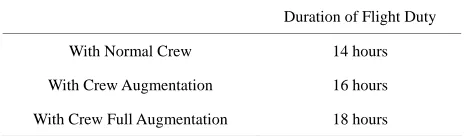
Duration of flight duties constitutes one of the funda- mental constraints in the airline crew scheduling process and is limited by regulations. All flight duties generated in the flight duty generation phase must fit the Crew and Duty Regulations of Directorate General of Civil Avia- tion [3]. The maximum duration time of a flight duty depends on the range of flights it contains, implemented crew model (time period might be increased with crew augmentation), and number of landings. The time periods of normal and extended range flight duties can be seen in Tables 2 and 3 [3]. According to the regulations, for a flight duty to be accepted as an extended range flight duty, 4 hours of time slice or 8 hours of flight time must be passed.
Table 1. Sample flight duty.
Duty Start
Duty End
Departure Time
Arrival Time
Dep. Airport
Arr. Airport 25.03.07
06:20
25.03.07 07:35
25.03.07
10:45 IST GVA
25.03.07 11:45 25.03.07 14:45 GVA IST
25.03.0716:00 25.03.07 17:00 IST ESB
[image:3.595.308.539.247.315.2]25.03.07 19:30 25.03.07 18:00 25.03.07 19:00 ESB IST
Table 2. Maximum duration of normal flight duty.
[image:3.595.307.540.347.415.2]Flight Duty Start Time 1 - 4 Landings 5 Landings 05.00 - 14.00 14 hours 13 hours 14.01 - 17.00 13 hours 12 hours 17.01 - 04.59 12 hours 11 hours
Table 3. Maximum duration of extended range flight duties.
Duration of Flight Duty With Normal Crew 14 hours With Crew Augmentation 16 hours With Crew Full Augmentation 18 hours 3.2. Rest Period
Rest period is the time period that starts after a flight duty and crew would be free for all kind of duty when they were in. The minimum duration of rest periods are showed in Table 4 [3].
3.3. Crew Pairing
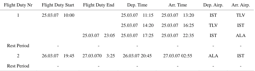
A crew pairing is a sequence of flights which begins and ends at a particular crewbase and consists of one or more flight duty(s). Unlike flight duties, crew pairings include rest periods. According to the regulations, a crew mem- ber cannot be away more than 10 days [3]. Therefore a crew pairing cannot last more than 10 days. A sample crew pairing which consists of two flight duties and four flights can be seen in Table 5.
3.4. Dead-Head Flight
Table 4. Minimum duration of rest periods.
Duration of previous flight duty Min rest duration
Until 6 hours 8 hours
Until 11 hours (included) 10 hours
Over 11 hours 12 hours
Between 12 - 14 hours or more than 3 hours of Time Zone Variation 14 hours For Extended Rage FlightDuties 2 local night/36 hours
Table 5. Sample crew pairing.
Flight Duty Nr Flight Duty Start Flight Duty End Dep. Time Arr. Time Dep. Airp. Arr. Airp. 1 25.03.07 10:00 25.03.07 11:15 25.03.07 13:20 IST TLV
25.03.07 14:20 25.03.07 16:25 TLV IST
25.03.07 23:05 25.03.07 17:25 25.03.07 22:35 IST ALA
Rest Period - - - -
2 26.03.07 19:45 27.03.070 3:25 26.03.07 20:45 27.03.07 02:55 ALA IST
Rest Period - - - -
when there is a crew member who has to fly to another airport to complete a flight which starts from that airport.
4. Solution of Crew Pairing Problem
Generally, the crew pairing problem is solved in two phases because of the large size of search space (as can be seen in references [6] and [7]), and the constraints which convert the problem to a highly constrained non- linear optimization problem and objective function are satisfied.
1) Crew pairing generation: In this phase, many legal crew pairings are generated using the airline’s timetable; for each crew pairing necessary values are carried out that will be used in calculating the objective function. There are some constraints that must be taken into ac- count for crew pairings to be considered legal crew pair- ings. While some of these constraints are spatial and temporal constraints, the rest of them are originated from Crew and Duty Regulations of Directorate General of Civil Aviation [3] or special implementations of the air- line company itself.
2) Optimization: Among crew pairings generated in the previous phase, subsets of crew pairings are searched which minimize crew costs and cover all flights in the schedule at least once (over-covering indicates dead-head flights).
The advantage of this approach is that the constraints are taken into account only during the first phase. There- fore the optimization becomes independent of constraints. In fact, once a large-size set of legal pairings has been
generated, the second phase can be modelled as a set covering problem, a widely known combinatorial opti- mization problem [7].
4.1. Crew Pairing Generation
Input data of the crew pairing generation process is the set of flightsFwhich is taken from airline flight schedule. System constraints are defined as a function
: 2F 0,1
C . Here crew pairing p is a legal crew pair- ing if C p
1 and is not legal if . The pur- pose of this phase is to obtain a set of all feasible crew pairings
0C p
2F C p 1
P p [7].
Considering the size of the problem however, it is not efficient nor is it possible to enumerate all feasible crew pairings. For instance if then it requires 21000 crew pairings be evaluated. At the same time, generation of too many crew pairings naturally increases the diffi- culty of the optimization phase. Therefore, in this phase as few crew pairings as possible are generated which allows preservation of the robustness and the quality of the solution.
1000
F
is repeated for every crewbase for a multibase solution. 4.2. Optimization
In the optimization phase, subsets of crew pairings which satisfy all crew needs and minimize the objective func- tion are searched among generated crew pairings created in the previous phase. This process should be modelledas a set-covering problem and solved with genetic algo- rithms.
If one considers that F is the set of flights which ap- pears in the flight schedule and P is the set of crew pair- ings, then the set-covering model for crew pairing prob- lem can be formulated as follows [14].
min p p
p P
c x
(1a):
1
p p i p
x i F
(1b)
0,1 px pP (1c) In the Equation 1(a), cp indicates cost value for each
crew pairing in P and xp is the decision variable which
indicates whether the crew pairing is in the solution set. Hence, Equation 1(a) gives the total cost of the solution. Equation 1(b) is an inequality constraint which guaran- tees the full covering of all flights in F. If Equation 1(b) gives a value greater than 1 for a flight in F in other words if the solution set has more than one crew pairing which covers a flight, that flight is a dead-head flight. Additional cost will be added for dead-head flights as described in fitness function section. And Equation 1(c) represents standart constraints for the problem.
Widely used methods for solution of set-covering problem are branch and bound based methods and ge- netic algorithms. Although branch and bound based me- thods could converge to more exact values, set-covering problems of a medium sized airline company may have approximately 5000 of rows and 100,000 of columns. Because of the nature of the problem, approximate me- thods (like in reference [15]) are developped. With this kind of method a much higher convergence rate is ob- tained for the solution of very large problems like 10000 of rows and 1,000,000 of columns. Genetic algorithms are comparatively powerful candidate in approximate opti- mization methods.
Unlike other genetic implementations, a new genetic operator—called perturbation operator—is implemented. As can be seen in the experimental results section, by using this operator, the convergence rate has been greatly increased.
4.3. Chromosome Representations for the Set-Covering Problem
Two kind of representations are suggested for using ge-
netic algorithms to solve the set-covering problem. These are column-based representation and row-based repre- sentation.
In column-based representation, chromosomes are rep- resented through a binary coded string that is composed of one or zero values. In this representation, each crew pairing is represented by a gene and each gene that could take values of one or zero that indicates whether the par- ticular crew pairing would be in the solution. The only disadvantage of this representation scheme is the infeasi- ble chromosomes that would be formed as a result of genetic operations. Hence, a heuristic feasibility operator has been implemented (in [4]) to cope with this problem.
In row-based representation, the number of genes that chromosomes include is equal to the number of flights. The index of each gene represents the flight and the value of each gene represents the crew pairing which covers the flight. However, in this method it is possible to represent the same solution in different forms because the same crew pairing would be represented by more than one gene. This situation makes the calculation of fitness function ambigious and enables different forms of chro- mosomes to generate the same solution and fitness va- lue.
Another disadvantage of this method is that the uni- form crossover operator, which gives good results in col- umn-based representation, results in too many dead-head flights. This situation might be solved with usage of one or multipoint crossover operators, nevertheless these me- thods do not give satisfactory results compared to the other method. Likewise, the mutation operator which is applied by changing some genes on the chromosome, increases the number of dead-heads. (See reference [10] in which an implementation of row based representation was studied.)
In this study, column based representation is used and results are improved by using additional genetic opera- tors.
4.4. Generation of First Population
The first phase of the genetic optimization is the popula- tion generation process. In order to carry out this process, a random crew pairing assignment should be done for each flight. Unlike study [4], in this study, if there were a flight that had been covered by a crew pairing which had been previously added to the solution, no crew pairing search would be done for this flight. In this way, low numbers of dead-head flights can be obtained. This process can be outlined as follows:
If
Set of all flights rows
F
Set of all crew pairings
P
columns
Set of crew pairings which covers flight ,
f f f F
Set of flights which are covered by ,
p p p P
Set of pairings which constitutes a solution,
S
SP
f fF
Number of pairings in S which cover flight ,
wf
Then
1) Set initial values S0 and wf 0 For each in :
2) f F
a) If wf 0 then goto 2 for next step 0; Select a pairing from p randomly
f
w
b) f ;
c) Add crew pairing to p S; d) wf wf 1, f p.
During the generation of the first population and the next, the iteration phases algorithm always checks to avoid existence of identical chromosomes in the same population. The population size for the crew pairing so- lution was determined as 20. The augmentation of the number of chromosomes may decrease the number of iterations but it does not provide a decrease in total solu- tion time because it raises the calculation times. After the generation of each chromosome of the initial population using the methods previously mentioned, the genetic algorithm becomes ready to run.
4.5. Genetic Iteration
After the generation of the first population, the main loop of the genetic algorithms is entered and selection, cross- over, mutation, and feasibility operators are applied re- spectively. During these processes, the similar operators which are presented in study [4] are implemented with some modifications.
First, the chromosomes which are used in the cross- over operator for reproduction are determined with the selection operator. In the presented work, binary tourna- ment selection is used for the selection operator because it does not need much in terms of extra calculation and runs fast. In this method, two sets which include two chromosomes are composed randomly and one in each two chromosome which has better fitness is chosen for the crossover phase.
Crossover operator can be considered as the transition phase by which the genetic information is passed to new generations, namely child chromosomes are generated in the phase. One or two child chromosomes (depending on the crossover operator implemented) are generated through the crossover operator which is applied to chromosomes of good quality which are taken from the previous popu- lation. The fusion crossover operator (which uses fit- nesses of chromosomes in a probabilistic way to select genes during crossover operation) is implemented. (The detail of the method can be found in study [4].)
The mutation operator is applied to child chromo- somes which are generated in the crossover process to avoid premature convergence; this provides a random search mechanism on a small scale. Usually, it is applied
as changing a certain number of genes with a small probablity. In reference [4], it is stated that the use of a variable mutation rate, which is increased with the con- vergence, gives much better results compared to using a fixed mutation rate. The convergence rate always de- creases while the algorithm approach to the optimum solution. Then progress provided by the mutation rate becomes more important than the progress provided by the crossover operator. The number of genes, which will be mutated, nm, is calculated by the Equation (2),
1 exp 4
f m
g c f
m n
m t m m
(2)
mf: Maximum value of variable that mutation rate can be.
mc: Iteration step when the variable mutation rate reached to the half of its maximum value.
t: Iteration step (Number of children which are gen- erated from the beginning).
mg: Gradient of the function at tmc.
In this study, mf ChromosomeLength 90, 200
c
m , mg 0.4were chosen.
After deciding the number of genes that would be mu- tated, another parameter which has to be decided is the mutation rate m. If a gene were selected to be mutated,
the mutation operator would be applied with the probab- lity m. The value of m is determined by the ratio of
the number of genes which are equal to 1 in the fittest individual of the population and the total length of chro- mosome (as stated in the study [7]). For instance, if a chromosome had 10 crew pairings in the solution over 100 crew pairings then m would be
o
o o
o om10 1000.1. If K is the chromosome which would be mutated and
is the length of the chromosome then the mutation operator works like this:
n
1) i1;
2) Choose an integer value from 1 to randomly for n x; If xn then i i 1 and goto 2
3) m ;
Choose a random real number betw
4) een 0 and 1 for y; 5) If [ ]K i 0 and yom thenK i
=1;6) If [ ] 1 and K i yom then K i
0; 7) i i 1 and goto 2.As stated in previous sections, until now there has been no guarantee about feasibility of chromosomes which are generated or modified by the genetic operators. Therefore a heuristic-based repair operator, called feasi- bility operator, is used to repair this kind of chromo- somes. (For details reader can consult studies [4] and [7]).
4.6. Perturbation Operator Implementation
the feasibility operator in order to enhance the efficiency of the current solution. In this operator, first, the chro- mosome is made infeasible through the removal of one or more crew pairings which are in the solution. Next alter- nate lower costs of crew pairings are searched on the chromosome to substitute removed ones to make chro- mosome feasible like feasiblity operator. This method is called the perturbation operator because chromosomes are made infeasible deliberately. If the search is success- ful then alternative crew pairings are taken into the solu- tion; if not the chromosome is reverted. The iteration process can be summarized as follows:
If
Set of all flights
F
Set of crew pairings which cover flight ,
f f f F
Set of flights which are covered by pairing ,p p P
p
Set of pairings which constitute a solution,
S
Set of uncovered flights,
U UF
S P
Cost of chromosome before pertur
C bation
Cost of chromosome after perturbation
C
Set of pairings which makes chromosom
L e feasible
Then
1) Calculate C 2) For each in :p S
– ;
a) SS p U U p
For each in f U: ; b)
i) Find the first crew pairing p'f, 'p p which minimizesratio cp Up
; ; ii) S S p L L p U U p
c) Calculate C;
d) If CCthen S S L S; S p; If CCthen CC
e) ;
f) Empty the sets and L U .
This operator is applied with a probability of approxi- mately 0.2 to one randomly selected child after the feasi- bility operator. The effect of this operation can be seen in the experimental results section. It can also be observed that the genetic algorithm could reach much better solu- tions in much less iteration and obtain much more robust and stable results in spite of the randomized nature of genetic algorithms.
Furthermore, in step 2, the perturbation operator is ap- plied with dual or trine combinations of crew pairings instead of singular implementation. However, search for the dual or above combinations substantially increases the iteration time compared to singular implementation. Nevertheless, dual or trine implementation of the pertur- bation operator can be used with a small probablity in the main loop of genetic algorithm or can be applied at the end for the best solution. Even better results can be ob- tained in this way.
4.7. Fitness Function
Another important issue that has to be determined is the
fitness function and the quantities which will be used instead of cost values in this function. Generally, total monetary cost is calculated (like in studies [6] and [1]). First, the cost of each crew pairing in the solution is cal- culated using the sum of crew salaries for the trip, hotel costs, etc. Then the total cost of of the solution can be calculated by adding these crew pairing costs.
But, as is stated by the crew scheduling department of Turkish Airlines (THY), the minimization of total dura- tion of crew pairings (flight duties + rest periods) was more important than the minimization of total monetary cost. Based on this requirement, in this study the total duration of crew pairings is used instead of monetary cost in fitness function. Regarding this requirement, all terms in fitness function are designed to produce dura- tion-based values.
Another point that must be taken into account is dead- head flights. The proportion of dead-head flights in the fitness function is mutiplied by a coefficient to minimize the numbers of flights because of their attenuator effect on the transportation capacity as stated in previous sec- tions.
Like dead-head flights there is another factor that must be considered and that is the crewbase distribution of crew members. Duty distribution of crewbases has to be proportionate to the number of crew who could be util- ized for each crewbase hence crew pairings have to be chosen in order to provide a regular work balance be- tween crewbases. This cost factor is very important for efficient duty assignment for crewbases. The fitness function which is used in this study (Equation (3)) and its paremeters are as follows:
: Cost value of i th crew pairing
pi
c
: If 1 then i th pairing is in th
g g
;
e solution otherwise not;
i i
: Cost of j th flight
fj
c
:Number of deadhe
d
;
ad status of j th flight
f j
: Total cost of pairings which belong to k th
c
; crewbase k
: Total cost of crew pairings
c
;
t
: Number of available crew w
e
;
ho resides in k th base k
: Number of total crew
e
;
t
: Deadhead penalty co
p ; efficient d ; then
Fitness Value . . . .
pi i f j f j d
i j
k k t k t
k
c g c d p
c c c e e
(3)The first expression in the equation gives the total cost of the crew pairings in the solution—called plain cost.
The second term in the expression is a penalty factor for the flights which are covered by more than one crew pairing (dead-head flights). In this term, the penalty co- efficient b has been applied for dead-head flights. (It
might be thought that dead head flights are already cov- ered by more than one crew pairing and the cost of the flight itself would already appear in these crew pairings more than one time). But there are additional cost factors inherent in deadhead flights including transport capacity and crew utilization reduction. So there is a requirement of additional cost calculation for other cost factors we could not calculate in the first term. In this presented work for experimental results, were chosen.
p
3
d
p
The last term in the expression of fitness function is the crewbase distribution cost which means work balance irregularity. Making proportional duty distribution is very important for efficient crew utilization and for mi-nimizing overtime crew costs. This is done by apply- ing a penalty factor that resides in the ratio difference be-tween total crew pairing duration and the total number of available crews. The number of the total available crew must be proportionate to the total crew pairing du- ration for a selected crewbase. For example if = 3500 hours,
hours, and t then the pen-alty coefficient for the crew distribution cost will be
k
c
80 10000
t
c ek 20 e
3500 10000
20 80
0.1. This means crew dis- tribution cost of the crew pairings which belong to a se- lected crewbase will be plain cost * 0.1. This increases the plain cost of the solution by 10 percent.Fitness function integrates three different but depend- ent objectives. These include minimization of total crew pairing cost, minimization of dead-head flights, and mi-nimization of crewbase distribution cost.
4.8. Population Replacement
The last step of the genetic algorithm is the population replacement phase. In this phase, we decide how to use the chromosomes that are generated and enhanced and how to apply genetic operators. For the solution proce- dure developed here, the elitist strategy has been used and the order of sequences is as follows:
1) Parents and children are composed in one popula- tion;
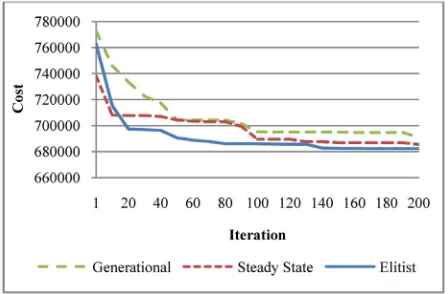
2) New population is ordered according to fitness; 3) First 20 chromosome are kept for next round. Furthermore, except for the elitist strategy two more approaches were tested. The first one is the generational approach which is based on all parents were replaced by children and the second one is the steady-state approach which is based on each child chromosome was replaced with a parent which has been selected according to fit-
ness randomly. But elitist strategy gives better results. The test results can be seen in Figure 1. Figure 1 was obtained for the first 200 iterations for just viewing pur- poses. However, for 10,000 iterations results are similar.
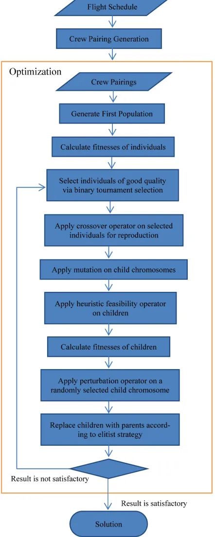
The general schema of genetic iteration is as in Figure 2.
5. Experimental Results
The presented test results were generated under Java NetBeans platform via java codes which were developed for this study. Test hardware was an AMD Athlon 1.8 MHZ single processor machine.
The test data used were taken from the flight schedule of THY (Turkish Airlines) which starts at 25th of March 2007 and ends at 11th of May 2007 (can be found in ref- erence [16]). Flight timetable of Airbus 315 fleet which includes 710 flights was selected as test data. After pair- ing generation 3308 pairings were generated before op- timization phase. It is also assumed that there were two crew bases. One sixth of all crews were considered as located in the first crew base and the rest were consid- ered as located in the second one.
There were four approaches tested. The first is genetic algorithm developed by Beasley and Chu (this approach will be called GA). The second is the genetic algorithm with perturbation operator (called GAPO). The third is the genetic algorithm approach suggested in study [12] (called GA-UnEx). The fourth approach is an exact me-thod based on branch and bound technique with dual simplex algorithm. This last approach gives us exact glo- bal optimum for the problem. By using this exact result we are able to evaluate solution qualities of genetic ap-proaches. The exact cost value of the studied dataset was found as 679,005 in 6 mins and 7 secs by using B&B with dual simplex method. While six minutes might look acceptable, the calculation time for the exact methods dramatically increases with the problem size increase.
[image:8.595.311.535.569.716.2]There are some abbreviations used in the result tables
Figure 2. General schema of the system.
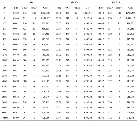
[image:9.595.62.283.91.641.2]to increase readibility. These are given in Table 6. Table 7 includes values of important optimization pa- rameters at particular iteration steps. Each of three ge- netic approaches were run for 10,000 iterations. As can be seen in Table 7, GAPO is capable of reaching much
Table 6. Abbreviations.
Term Abbreviation Genetic Algorithm with Perturbation Operator GAPO
Genetic Algorithm approach of study [12] GA-UnEx Branch&Bound with Dual Simplex B&B
Iteration Itr Number of Crewpairings NoCP
Number of Deadheads NoDH
better results in much less time.
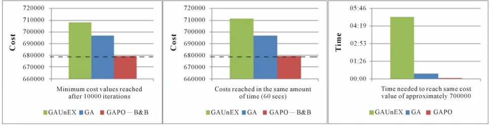
Graphical representations of the results can be seen on Figures 3 and 4. As was mentioned in previous sections because of additional perturbation operators, GAPO needs more calculation time for just one iteration than GA. However, it can converge much faster and total necessary runtime will be much less than GA. GA-UnEx is especially useful for decreasing deadheads, but be- cause of the greedy approach, it is computationally more expensive than either GAPO and GA. Please note that the line represents B&B algorithm shows the final cost value (679,005) we got by using it. It is put for us be able to compare solution quality of other GA implementa- tions.
6. Conclusions and Future Work
In the presented work, airline crew pairing problem is revisited. In terms of crew scheduling problems, crew pairing optimization is the main cost-determining phase. Since crew pairing costs are the second largest opera- tional cost, after fuel costs, well-arranged crew distribu- tion flights might surely increase utilization of the crew and benefit for the airline.
During the development of the presented solution pro- cedure, existing methods were examined, adapted, and improved. Scenarios with multiple crewbases were also simulated using genetic algorithms. From the results ob- tained one can deduce an incremental increase in con- vergence rate as well as an incremental increase in ro- bustness applying this new procedure. The perturbation operator implementation has great effect on having this fast and robust convergence. Additionally, the number of dead-head flights is reduced through the application of the strategy developed during the population generation phase. This reduction has a direct effect on the total cost.
Monetary benefit of the results of the new imple- mented perturbation operator can be calculated with the multiplication by a monetary coefficient because the terms used in fitness function were duration related terms.
Figure 3. Convergence comparison of applied algorithms.
Table 7. Solution comparison.
GA GAPO GA-UnEx
[image:10.595.58.538.308.737.2]Figure 4. Comparisons in various aspects.
the success of the crew rostering phase is completely de- pendent on the quality of the results of the crew pairing phase.
The usage of larger populations and perturbation op- erator with higher probablity ratio can make the algo- rithm more effective. But in this situation, the run time increases because of the required increase in calculation time. Distributed genetic algorithms can be proposed as a direction for future work to be able to use much larger populations without increasing calculation time.
REFERENCES
[1] H. T. Ozdemir and C. K. Mohan, “Flight Graph Based Genetic Algorithm for Crew Scheduling in Airlines,” In-
formation Sciences, Vol. 133, No. 3-4, 2001, pp. 165-173.
doi:10.1016/S0020-0255(01)00083-4
[2] F. M. Zeghal and M. Minoux, “Modeling and Solving a Crew Assignment Problem in Air Transportation,” Euro-
pean Journal of Operational Research, Vol. 175, No. 1,
2006, pp. 187-209.doi:10.1016/j.ejor.2004.11.028
[3] Republic of Turkey Ministry of Transport, Maritime Af- fairs and Communication, “Instruction on Flying Team’s Task and Resting Terms and Principles of Application,” 2005. http://www.shgm.gov.tr/doc3/sht6a50.doc
[4] J. E. Beasley and P. C. Chu, “A Genetic Algorithm for the Set Covering Problem,” European Journal of Opera-
tional Research, Vol. 94, No. 2, 1996, pp. 392-404.
doi:10.1016/0377-2217(95)00159-X
[5] J. H. Holland, “Adaptation in Natural and Artificial Sys- tems,” MIT Press, Cambridge, 1975.
[6] C. P. Medard and N. Sawhney, “Airline Crew Scheduling —from Planning to Operations,” 2005.
http://www.carmen.se/research_development/research_re ports.htm
[7] H. Kornilakis and P. Stamatopoulos, “Crew Pairing Op-timization with Genetic Algorithms,” Lecture Notes in
Computer Science, Vol. 2308, 2002, pp. 109-120.
doi:10.1007/3-540-46014-4_11
[8] C. Barnhart, et al., “Branch-and-Price: Column Genera- tion for Solving Huge Integer Programs,” Operations
Re-search,Vol. 46, No. 3, 1998, pp. 316-329.
doi:10.1287/opre.46.3.316
[9] D. Klabjan, E. L. Johnson and G. L. Nemhauser, “Solving Large Airline Crew Scheduling Problems: Random Pair- ing Generation and Strong Branching,” Computational
Optimization and Applications, Vol. 20, No. 1, 2001, pp.
73-91. doi:10.1023/A:1011223523191
[10] L. F. G. Hernandez, “Evolutionary Divide and Conquer for the Set-Covering Problem,” Lecture Notes in Computer
Science, Vol. 1143, 1996, pp. 198-208.
doi:10.1007/BFb0032784
[11] U. Aickelin, “An Indirect Genetic Algorithm for Set Cov-ering Problems,” Journal of the Operational Research
So-ciety, Vol. 53, No. 10, 2002, pp. 1118-1126.
doi:10.1057/palgrave.jors.2601317
[12] T. Park and K. R. Ryu, “Crew Pairing Optimization by a Genetic Algorithm with Unexpressed Genes,” Journal of
Intelligent Manufacturing, Vol. 17, No. 4, 2006, pp. 375-
383. doi:10.1007/s10845-005-0011-z
[13] L. H. Lee, C. Ung Lee and Y. P. Tan, “A Multi-Objective Genetic Algorithm for Robust Flight Scheduling Using Simulation,” European Journal of Operational Research, 2007, Vol. 177, No. 3, 2007, pp. 1948-1968.
doi:10.1016/j.ejor.2005.12.014
[14] C. Barnhart, A. M. Cohn, E. L. Johnson, D. Klabjan, G. L. Nemhauser and P. H. Vance, “Handbook of Transporta- tion Science,” Springer, Berlin, 2003.
[15] D. Wedelin, “The Design of a 0-1 Optimizer and Its Ap-plication in the Carmen System,” European Journal of
Operational Research, Vol. 87, No. 3, 1995, pp. 722-730.
doi:10.1016/0377-2217(95)00243-X