Valve vs. solid-state microphone preamplifier: a comparative study
Octavian Stroe
Email: [email protected]
Abstract
This paper outlines research carried out to determine the perceptual and objective differences between a solid-state and a valve preamplifier running at low voltages. ABX testing was employed and showed that there were perceivable differences between the two systems. A comprehensive objective analysis was performed, which utilised tests for total harmonic distortion + noise (THD+N), intermodulation distortion (IMD), THD versus frequency and frequency response in order to ensure the two systems were performing in their linear region. In addition, MIRToolbox was utilised to extract low-level features such as spectral centroid, skewness and novelty. The electronic
measurements combined with the MIRToolbox support the listeners’ subjective descriptors that there is a difference in brightness and harmonic content between the two types of preamplifiers. A correlation theory was developed, which linked the objective and the subjective measurements.
Keywords: Valves; solid-state; preamplifiers; objective and subjective measurements; THD+N; IMD; spectral centroid; skewness;
Introduction
Within the audio industry there are ongoing and controversial debates over the
differences in tonality and perceived sound quality of valve and solid-state amplification. Microphones are connected to a preamplification stage and the choice of this stage is an important part of the signal chain.
Circuit design
Two preamplifiers were built, one based around a solid-state design, the other valve based. Both circuits utilised identical input and output stages to try to ensure any perceptual differences were due to the amplification stage only.
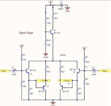
Input stage
The input stage (Figure 1) features an electronically balanced input, with a transistor long-tailed pair, with constant current source on the collector and a PNP complementary feedback pair.
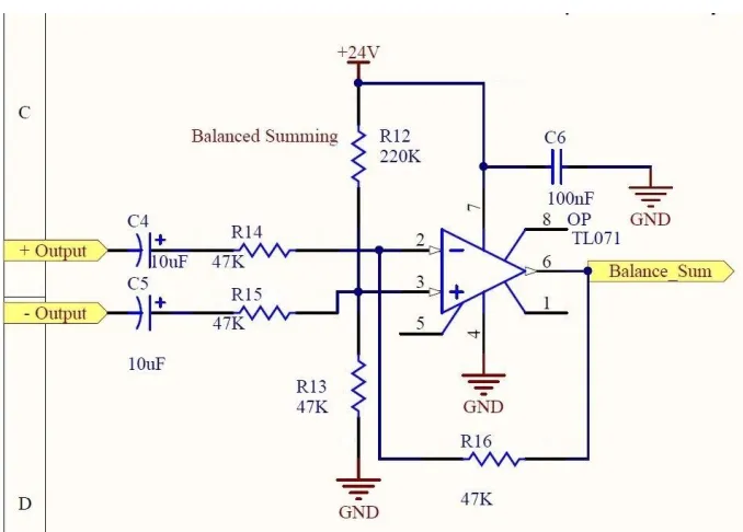
Figure 2: Summing Op-Amp
The stage presented in Figure 2 has the role of summing the signals from the buffer, converting them into a single-ended output.
Amplification stage
Solid-state
In both cases, the amplification stages (Figure 3 and Figure 4) are kept as similar as possible in order for the results to be comparable, so both preamplifiers feature a two-stage amplification topology, AC coupling, adjustable gain and a similar number of components.
Valve
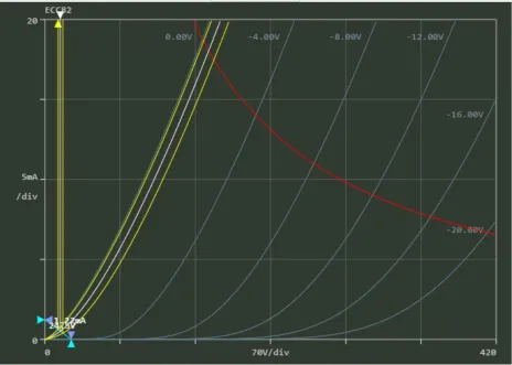
All the working currents were obtained using the load-line from Figure 5, provided by Makarewicz (2014).
To allow for signal headroom, a grid bias voltage of −0.5V was chosen, which, in theory, allows for inputs of up to approximately 500mVp-p, with the result that the cathode had to be biased at 0.5V. Based on the load-line, when the swing pulled the anode at 0V, resulting in 24V across the anode resistor, the maximum flowing current would be 1.22mA.
By using the load-line, the transconductance, plate resistance and amplification factor were calculated according to Elliot (2009) and represent the DC quiescent condition:
𝑔𝑚 = ∆𝐼
∆𝑉= 0.7−0.2 1𝑉 = 0.5𝑚𝐴 1𝑉 = 500µ𝐴
𝑉 = 500µ𝑚ℎ𝑜𝑠 – calculated at constant plate
voltage
𝑟𝑝 =∆𝐸𝑝
∆𝐼𝑝 =
24−12
1.22−0.2=
12
1.02= 12𝑘Ω - calculated at constant grid voltage
µ = 𝑔𝑚 ∗ 𝑟𝑝 = 6.3 𝐴𝑣 = 4.15/𝑡𝑟𝑖𝑜𝑑𝑒
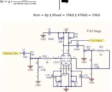
𝐴𝑣 = µ ∗ 𝑅𝑡𝑜𝑡
𝑟𝑝+𝑅𝑡𝑜𝑡+(µ+1)∗𝑅𝑘
𝑅𝑡𝑜𝑡 = 𝑅𝑝 ∥ 𝑅𝑙𝑜𝑎𝑑 = 19𝑘Ω ∥ 470𝑘Ω = 19𝑘Ω
Figure 5: Valve Load-Line
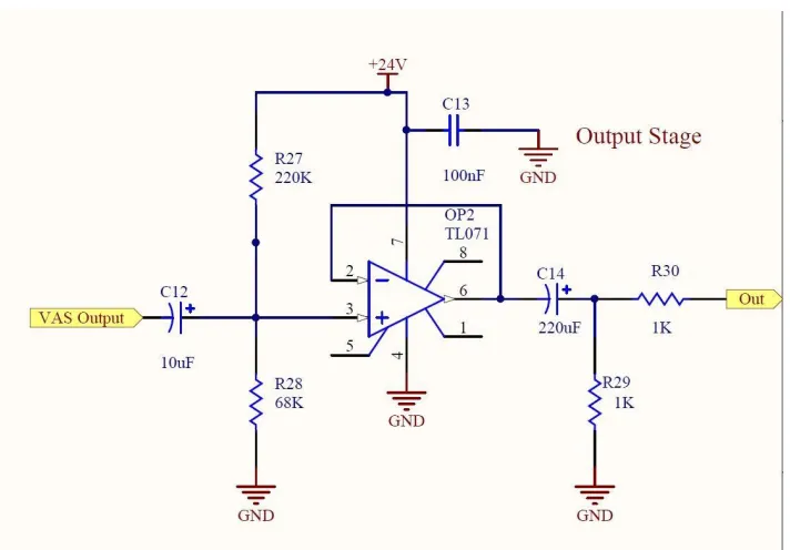
Output stage
The output stage that can be seen in Figure 6 features an op-amp in voltage-follower configuration used primarily to convert a high-input impedance to a low-output
Figure 6: Output Stage
Key audio measurements
Objective measurements
Objective measurements employed in this study consisted of both electronic
measurements and the use of a low-level feature extraction tool called MIRToolbox (Lartillot, 2013).
All electronic measurements were carried out using a PRISM dScope III audio analyser, and parameters Total Harmonic Distortion + Noise (THD+N), intermodulation distortion (IMD), individual harmonic magnitude and frequency response were measured. The systems were tested for their transient response using a square wave generator. All measurements were taken under a load of 10kΩ.
The THD parameter is one of the most important as it provides information on the harmonic distortion of a system over the gain range or the frequency range and is used to characterise the linearity of audio systems and the power quality of electric power systems. As noted by Metzler (1993), it is a measurement of the harmonic distortion present in the system and is defined as the ratio of the sum of the powers of all harmonic components to the power of the fundamental frequency.
The first three harmonics were also measured individually for each preamplifier, as they are the most representative, having the highest distortion values and theoretically being responsible for any perceived differences.
The frequency response factor can add to the sound timbre depending on the amplitude of certain frequencies, and can introduce perceivable differences if one lacks
low-frequency response or high-low-frequency response.
As Elliot (2012) specifies, the IMD test is more meaningful than a THD analysis because it gives the distortion values for the products which are not harmonically related to the pure input signal. The Society of Motion Picture and Television Engineers (SMPTE) specifies the two signals to be at 60Hz and at 7kHz which are summed at a 4:1
amplitude ratio (12dB ratio), as described by Bohn (2000). Metzler (1993) summarises IMD as the amplitude modulation of signals containing two or more frequencies, which is caused by having a non-linear behaving system.
Square wave testing is very meaningful for checking the system’s transient response according to Elliot (2015), being particularly suitable for correlating the findings with the spectral centroid or the skewness, tests that are presented below.
Using MIRToolbox, attack slope was measured in order to detect the attack/rise times of the notes played on an instrument. This test, together with the novelty curve, is used to determine whether there are any differences in transient response of the two
preamplifiers. Spectral centroid measure was carried out, as recommended by
Zacharov and Bech (2006). The test looks into the shape of a distribution through the use of its moments, and is a measure that has been shown to relate to the perceived brightness of an audio signal. Skewness was also measured, from which transient response can be predicted, by identifying where the most energy is centred, depending on the skew, which can be either positive or negative.
Listening experiment
Proposed stimuli
Four samples were utilised for testing. A piano was used for its rich harmonic content, an electric bass for the low frequencies, and a guitar with simple struck chords for its envelope characteristics and high number of harmonics distribution. In addition, a cello was used for its sustained notes to see how the system reacts to constant energy levels, the difference between the cello and bass samples being the higher harmonics distribution of the former. All samples utilised in the testing were loudness normalised using a ITU-1770-4 standard loudness meter.
Test method
An ABX testing method was used for this project, in line with the ITU BS.1116
sample was which. The subjects were also given another stimulus, X, which was
chosen randomly from either A or B, and were asked to say if X was A or B. In order for the measure to be considered valid, the subjects underwent 10 trials per set of samples to ensure that the final result was neither random nor based on luck. The subjects did not know what the test was investigating, or that samples A and B were different, thus reducing biasing effects. Also, the afferent deviation was calculated according to instructions provided by Koch (n/a)
After the test had ended, the subjects were asked to comment on the main differences perceived between the solid-state and the valve sound (as they were told at the end which was which). From this, a list of descriptors was collected.
Results
Subjective results
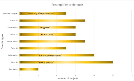
Figure 8: Listeners Preference and Descriptors Chart
Figure 8 summarises all descriptors that were provided by the listeners.
Objective results
THD+N
Values were measured for a 100mVp-p input at 1kHz with maximum gain and the results are shown in Table 1.
Valve
Preamplifier
Solid-State Preamplifier THD+N absolute, 100mV input, max gain −53.5dBu −58.7dBu THD+N relative, 100mV input, max gain 0.56% 0.136%
Table 1: THD+N levels for the two preamplifiers under test
Second, third and fourth individual harmonics
2nd Harmonic 3rd Harmonic 4th Harmonic
Valve −33.48 dB −34.04 dB −39.37 dB
Solid-state −39.25 dB −33.32 dB −34.66 dB
Frequency response
Figure 9: Solid-State Frequency response
IMD – SMPTE Standard
Valve preamp 0.03%, 60Hz,7kHz, 4:1 ratio, maximum gain
Solid-state preamp 0.0057% 60Hz,7kHz, 4:1 ratio, maximum gain
In-Out configuration 0.0055% 60Hz,7kHz, 4:1 ratio, maximum gain
Table 3: IMD Values
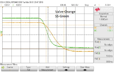
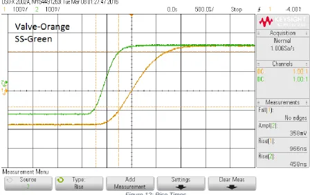
Square wave response
Figure 12: Rise Times
MIRToolbox measurements
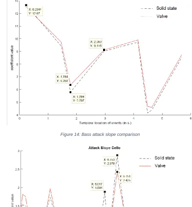
Attack slope
Figure 14: Bass attack slope comparison
Novelty curve
Figure 16: Piano novelty difference
Spectral centroid
Figure 18: Bass Centroid
Skewness
Figure 20: Bass Skewness
Analysis of results and correlation theory
First of all, it is important to discuss the results from Figure 7 and Figure 8. The poorer bass identification percentage was expected before testing because the bass is a stream of continuous energy with constant RMS, so there are no sudden changes that might trigger different preamplifier behaviour. However, some subjects were still able to identify the difference and also provided interesting comments on their perceived
dissimilarity. The biggest deviation from the mean can be seen in the bass sample. This can be explained with reference to the nature of human hearing, which is less sensitive to low frequencies, which do not, or should not, present any difference when they are reproduced by different systems. The cello sample presents the lowest deviation, even though the valve piano sample was subjectively regarded as being the brightest. This could be explained by the fact that the cello sample had just a couple of sustained notes, as opposed to the piano, which had many more notes played in the same period of time, thus preventing the listener from focusing on timbre. Therefore, listeners paid more attention to the character of the cello sample. But even though the deviation is quite large on the piano, taking into consideration the mean result and the subjective opinions provided by the listeners, the result can be regarded as significant and relevant.
The standalone THD+N measurements seen in Table 1 show a difference of
approximately 5dB between the valve and the solid-state preamplifier, a variance that cannot alone account for the brightness difference. Moreover, the individual harmonics presented in Table 2 show that the 3rd harmonic, which is usually regarded as non-musical, presents close values (within 1dB difference) for both preamplifiers, whereas the 2nd harmonic is higher for the valve preamplifier and the 4th harmonic is higher for the solid-state. The 5dB difference between the two cases could explain some of the difference in brightness. Figure 10 shows that the valve preamplifier presents a low- and high-frequency roll-off, which, in theory, would be equivalent to a boost in the
mid-frequencies. Taking into consideration the results from the frequency response and the individual harmonics tests, it can be stated as a first fact that the reported difference in brightness could be explained by these two factors.
Moreover, as Metzler (1993) specifies, the intermodulation distortion test is more
meaningful than a THD analysis as it gives the distortion values for the products, which are not harmonically related to the pure input signal. Table 3 shows that the valve’s IMD value is five times that of the solid-state, indicating that the content created by the non-harmonically related frequencies is much higher in the valve preamplifier.
So far, electrical measurements were taken into consideration, especially the THD measurements and it was concluded that one possible cause for the brightness could be the combined effects of frequency response, 2nd order harmonic and IMD.
preamplifier would suffer both low- and high-frequency roll-off, and this is proved by the frequency response graph.
More important in the square wave test are the rise and fall times, which give an indication of the transient response of the system, as stated by Elliot (2015). It can be seen from Figure 11 and Figure 12 that the solid-state exhibits faster rise and fall times, indicating a better transient response that is approximately equivalent to an amplifier’s slew rate. The difference in rise and fall times may explain some of the listeners’ claims of a difference in ‘drive’ and ‘attack’ of the notes. It can be explained by thinking of the higher inner capacitance which produces a higher Miller effect, the final total
capacitance being represented by the plate-grid capacitance from the datasheet
multiplied by the gain. Combining this theory with the information provided by the attack slopes in Figure 14 and Figure 15 and listeners’ comments from Figure 8, it can be concluded that, particularly for the bass, the difference arises from the different transient response of the two systems. Although the bass test shows a high deviation from the mean (see Figure 7), the test is still valid as the majority of participants could describe a difference between the two samples.
The novelty results from Figure 16 and Figure 17 also support comments such as ‘more attack’, ‘faster attack’ by showing that there are quite big differences between the two preamplifiers at the same moments of time. This contrast may be due to both the different transient response and the low-frequency roll-off exhibited by the valve preamplifier. Until now, based on the measurements taken, the ‘accuracy of reproduction’ claimed by five of the listeners who would choose the solid-state preamplifier for all the instruments can be attributed to the better overall frequency response, lower THD, lower IMD and better transient response of this preamplifier, which translates into a much cleaner, neutral sound.
The overall subjective increase in brightness for the valve preamplifier can also be acknowledged through the spectral centroid measurement. Figure 18 and Figure 19 show that in the case of the cello, the coefficient values for the centroid are greatly elevated, indicating that most of the energy at that particular instant of time was in the high-frequency register. The bass sample presents almost identical centroid
measurements for the preamplifiers, showing, as reported by the listening tests, that the bass is not brighter.
The transient response can also be estimated by looking at the skewness results (Figure 20 and Figure 21). It can be seen that in both cases, the skewness coefficient values are higher for the solid-state preamplifier, meaning that they are positively skewed with regard to the valve’s values. A positive skew means that the system
two inverse U shapes represent the strings being struckand, as in the case of the bass, an elevated skewness value can be seen. Therefore, the claim of ‘more drive’ can be proved. In the other samples, an overall accentuated coefficient value for the solid-state preamplifier was identified.
Correlation theory
During the analysis of both the subjective and the objective measurements, different aspects of the systems have been brought into the discussion. It has been seen that although the overall difference in THD+N between the two systems is only around 5dB, when the systems were tested for the evolution of THD over frequency, a much greater difference was identified. Moreover, in order to prove that frequency response does not have a high impact on the difference between the two preamplifiers, the original cello sample (the one used for recording through both preamplifiers) was equalised with a curve like the one in the valve’s response. Comparing the resulting equalised sample to the original in MATLAB showed a very slight difference in spectral centroid between the two. The difference alone could not be held responsible for the overall increase in brightness due to frequency response difference.
The increase in THD vs. frequency in the valve preamplifier can be attributed to the low working plate voltage, which is right at the bottom of the valve’s capabilities. Basically, the valve is near the edge of cut-off, but still working linearly for line-level amplification. Moreover, the IMD measurement, which indicates the distortion caused by the product of the non-harmonically related frequencies, shows that the valve produces 5.2 times more distortion than the solid-state. The IMD can be caused by the high internal
capacitance of the valve compared to the solid-state’s inner capacitances. By combining the increased THD, IMD and low- and high-frequency roll-off in the valve preamplifier, it can be concluded that these are the main differences that explain the overall increased brightness in the valve samples. The rise and fall times explain the better transient response in the solid-state preamplifier. The THD also explains one of the listener’s comments for the cello valve sample: ‘enhanced harmonics’. The reported brightness is also backed up by the spectral centroid tests.
Conclusion
This paper details a comprehensive set of tests to determine whether there are
perceptual differences between solid-state and valve preamplifiers. Both preamplifiers work according to the schematic’s calculations and in the linear region, ensuring that they can be fully compared. The results indicate that there are clear differences
between the two systems, and both the electronic and MATLAB measurements support the subjective findings reported by the listeners. An identification rate of 70%, and in some cases even above 90%, coupled with an extensive number of trials, proves that participants were able to tell the difference between valves and solid-state amplification at low voltages, the reasons being the increase in THD vs. frequency, IMD, frequency and transient response. Participants’ preferences regarding the two preamplifiers differed from instrument to instrument. While five people would choose the solid-state for all of the instruments, the other seven had split opinions over the preference for solid-state and valve, depending on the audio material. Six people would choose a preamplifier that brightens the piano, so chose the valve. The rich harmonic content of the cello led eight people to choose the valve preamplifier, as it enhances the
harmonics. Conversely, 10 people chose the solid-state for the bass due to the better transient response. The six people who chose the solid-state for the guitar reported that it had more drive, while the other seven felt that the valve enhanced the guitar’s body (500Hz – 1.5kHz).
Further work
The work carried out on this topic covers most possibilities extensively, but further work could be carried out in order to find more reasons for the differences between the two preamplifiers. The internal architecture of the valve could be further analysed to find out what differences there are in construction between the solid-state and the valve that could explain the dissimilarity.
According to previous research on this subject, there is a reported difference between the same valve model manufactured by different companies. Another enhancement to the project would be for both the input and output stages to be changed and replaced with matched pairs of transistors, which are usually available as a package (like
References
Bohn, D. (2000). Audio Specifications. Retrieved from http://www.rane.com/note145.html
Elliot, R. (2009). Valve (Vacuum Tube) Amplifier Design Considerations. Retrieved from http://sound.whsites.net/valves/design.html
Elliot, R. (2009). Valves (Vacuum Tubes) - Biasing and Gain. Retrieved from http://sound.whsites.net/valves/bias-gain.html
Elliot, R. (2012). Intermodulation - Something ‘New’ To Ponder. Retrieved from http://sound.westhost.com/articles/intermodulation.htm
Elliot, R. (2015). Squarewave Testing Of Amplifiers & Filters. Retrieved from http://sound.westhost.com/articles/squarewave.htm
Fazenda, B. (2014). How to Design and Conduct Listening Tests for Audio and Acoustics. Retrieved from
http://usir.salford.ac.uk/34338/1/Fazenda-
Uni%20of%20Salford%202015%20-%20How%20to%20Design%20and%20Conduct%20Listening%20Tests.pdf
International Telecommunication Union. (2015). ITU-R : BS.1116-3. Geneva: . Retrieved from http://www.itu.int/dms_pubrec/itu-r/rec/bs/R-REC-BS.1116-3-201502-I!!PDF-E.pdf.
International Telecommunication Union. (2015). ITU-R : BS.1770-4. Geneva: .
Retrieved from https://www.itu.int/dms_pubrec/itu-r/rec/bs/R-REC-BS.1770-4-201510-I!!PDF-E.pdf.
Koch, R. W. (n.d.). A tutorial in probability and statistics [Tutorial]. Retrieved from http://web.cecs.pdx.edu/~roy/tutorial/Stat_int.htm
Lartillot, O. (2013). MIRToolbox 1.5 User’s Manual. Retrieved from
https://www.jyu.fi/hum/laitokset/musiikki/en/research/coe/materials/mirtoolbox/MIRtoolb ox1.5Guide
Makarewicz, G. (2014). Triode/Pentode Loadline Simulator The Audio Critic. Retrieved from http://www.trioda.com/tools/triode.html
Metzler, B. (1993). Audio Measurement Handbook. USA Beaverton: Audio Precision.
Palmer, R. (2005). Audio power amplifier measurements, Part 2. Analog Applications Journal (Texas Instruments Incorporated). Retrieved from