!∀#∃∀∀#%&∋())∋∃∃∃∋∀#!
%∗%!+%∋% % %∋
&#∀%(,,∗!∗−,)./.,
Using Grey Relational Analysis to Predict Software Effort with Small Data Sets
Qinbao Song
∗, Martin Shepperd
†, and Carolyn Mair
‡Abstract
The inherent uncertainty of the software development pro-cess presents particular challenges for software effort pre-diction. We need to systematically address missing data val-ues, feature subset selection and the continuous evolution of predictions as the project unfolds, and all of this in the context of data-starvation and noisy data. However, in this paper, we particularly focus on feature subset selection and effort prediction at an early stage of a project. We propose a novel approach of using Grey Relational Analysis (GRA) of Grey System Theory (GST), which is a recently devel-oped system engineering theory based on the uncertainty of small samples. In this work we address some of the theoret-ical challenges in applying GRA to feature subset selection and effort prediction, and then evaluate our approach on five publicly available industrial data sets using stepwise re-gression as a benchmark. The results are very encouraging in the sense of being comparable or better than other ma-chine learning techniques and thus indicate that the method has considerable potential.
Keywords: software project estimation, effort prediction, feature subset selection, empirical evaluation, Grey Rela-tional Analysis, Grey System Theory.
1. Introduction
Software development, or our understanding of it, is a grad-ual and evolving process; we know less at the beginning than at the completion of a project. As the software devel-opment proceeds, we gather and analyze incomplete infor-mation and try to optimize the development process. But the optimization may not be unique, it is modified or changed as more information becomes available. This means that effort prediction methods must also be suitable for dealing with uncertainty and for continuous effort estimating.
At the same time, in this process, the relationship be-tween project effort and the feature subset that affects the
∗Xi’an Jiaotong University, P.R. China - [email protected] †Brunel University, UK - [email protected] ‡Brunel University, UK - [email protected]
effort is unclear or the relational information is incomplete1.
It can be difficult to select feature subsets and predict project effort with traditional statistical methods or machine learning methods. These methods usually require a large complete sample or data that follow a certain statistical dis-tribution. Unfortunately, current effort prediction methods do not properly take into account these critical character-istics of the software development process and the project data sets. Although there is a great deal of research activity on this topic, a wide range of prediction techniques are be-ing proposed and increasbe-ing numbers of empirical studies published, however, no one technique is consistently effec-tive, and the software industry does not have a good track record for accurate cost estimation with typically 75% of projects reporting overruns2. Therefore, we should
system-atically address effort prediction in the context of small, in-complete data sets, this includes missing data imputation, feature subset selection and continuous (or ongoing) effort prediction.
Grey System Theory (GST), a recently developed sys-tem engineering theory based on the uncertainty of small samples, was first developed by Deng in 1982 [8]. The sys-tem was named by using grey as the colour which indicates the amount of known information in control theory. For in-stance, if the internal structures and features of a system are completely unknown, the system is usually denoted as a ‘black box’. In contrast, ‘white’ means that the internal features of a system are fully explored. Between white and black, there is a grey system indicating that part of the in-formation is clear, while another part is still unknown.
GST has certain distinct advantages, such as having sim-ple processes to study comsim-plex systems and providing reli-able analysis results, and allowing us to utilize only a few known data to establish an analysis model. In the context of data-starvation, GST is known to be effective and has been successfully and widely applied to address the real world problems in image processing [15], mobile communication [26], machine vision inspection [13], decision making [17], stock price prediction [27], and system control [11]. GST
1Not all features (variables) that are available are useful and some may
not only be redundant, they may positively hinder the prediction task. Re-moving such features is known as feature subset selection.
is not based on statistical theory, thus only requires a lim-ited amount of data to estimate the behaviour of an uncer-tain system. We explore the GST-based approach to address project effort prediction questions.
In this paper, we focus on feature subset selection and effort prediction with between-project data sets at an early stage of a development process and leave the imputation and evolutionary aspects of prediction for future work. Fea-ture subset selection is the process of identifying and re-moving as many irrelevant and redundant features as possi-ble from an original feature set for the purpose of providing better prediction accuracy. It has been widely used to obtain predictive features without creating new features based on transformations or combinations of the original feature set. However, most of the feature subset selection methods are for classification tasks, and can give poor results when the sample size is small [12]. At the same time, software project effort is a continuous valued feature that makes classifica-tion methods generally inappropriate. Therefore, we seek to improve upon traditional feature subset selection methods. By analyzing the influence of various features on the con-tinuous values of project effort, GST can help us gain the most predictive feature subset from a small data set.
Grey Relational Analysis is a method of GST. We pro-pose a Grey Relational Analysis based software projeCt Effort prediction (GRACE) method including feature sub-set selection. Our experiments, using five publicly available real-world data sets, explore the advantages this new ap-proach might offer relative to existing methods.
The remainder of the paper is organized as follows. In the next section we present related work on software effort prediction. This is followed by the introduction of the Grey Relational Analysis (GRA) method and the GRA based ef-fort prediction method GRACE. After that, we describe the data sets, the validation method, and the evaluation criteria we used. The results follow with a concluding discussion and suggestions for further work.
2. Related Work
Machine learning methods have been used to predict soft-ware effort since the 1990s. A primary advantage is that they are nonparametric and adaptable, and many of them make no or minimal assumptions about the form of the function under study [25]. Of course, there are also prob-lems, not least that they are difficult to configure to new situations and there is little theory so that their application often becomes a matter of trial and error. The most com-monly used methods include case based reasoning (CBR), regression and decision trees, and artificial neural networks (ANN).
Mukhopadhyay et al. [21] presented early work using CBR. They used Kemerer’s data set [16] and found that
their analogy-based model Estor outperformed COCOMO [2]. Shepperd and Schofield [24] compared an analogy based method with stepwise regression (SWR) on nine dif-ferent industrial data sets and report that in all cases anal-ogy equalled or outperformed SWR. Finnie and Witting [10] compared CBR with different regression models us-ing function points (FPs) and ANNs. They report that CBR outperformed regression models based on function points. On the other hand, Briand et al. [5] and Jørgensen et al. [14] obtained conflicting results where the regression model generated significantly better results than a CBR ap-proach. Finnie and Witting [10] also found ANN outper-formed CBR.
Regression and decision trees are another method that has been used to predict software effort. Briand et al. [4] compared the optimized set reduction (OSR) strategy with COCOMO and SWR. They used the COCOMO81 data set [3] as a training set and the Kemerer data set as a test set. OSR outperformed COCOMO and SWR. Srinivasan and Fisher [25] illustrated the use of CARTX to predict soft-ware effort. They also used the COCOMO81 data set for training and the Kemerer data set for testing. They report that CARTX outperformed COCOMO and SLIM [22].
Witting and Finnie [28] report the use of back propaga-tion (BP) artificial neural networks (ANN) to predict soft-ware effort. Although the results are encouraging, unfortu-nately, the data sets were large and only a small number of projects were used for testing. Srinivasan and Fisher [25] found BP neural networks outperformed regression trees. Samson et al. [23] compared an ANN method with linear regression using the COCOMO81 data set. Although the ANN method outperformed the linear regression method, both methods performed badly.
For a more detailed review see Briand and Wieczorek [6]. Nonetheless, even this brief introduction to machine learning methods for software effort prediction reveals that the results are quite mixed. Apart from using different data sets and different experimental methods, these methods tend to borrow from other disciplines where large data sets are the norm or data that follow a certain statistical distribu-tion are necessitated. Our GRACE method is quite different from these methods; it is at least an alternative method for software effort prediction.
3. GRA Based Software Effort Prediction
3.1
Grey Relational Analysis
3.1.1 Basic Concepts
Factor space. Letp(X)be a theme characterized by a fac-tor setX, andQbe an influence relation, {p(X);Q}is a factor space. The factor space{p(X);Q}has the following properties:
• Existence of key factors, for example, the key factors for a basketball player can be height and rebound.
• That the number of factors are limited and countable.
• Factor independence, so each factor must be indepen-dent.
• Factor expansibility, so for example, besides the height and rebound, weight can be added as another factor.
Comparable series. Suppose xi =
{xi(1), xi(2), . . . , xi(m)}, where i = 0,1,2, . . . , n ∈ N;m∈N, is a series. This series is said to be comparable if, and only if, the following conditions are met:
• Dimensionless. Factors must be processed to become non-dimensional, irrespective their units and scales.
• Scaling. The factor valuexi(k)(k = 1,2, . . . , m)of
different seriesxi(i = 0,1,2, . . . , n)must be at the
same level.
• Polarization. The factor value ofxi(k)of different
se-riesxi(i = 0,1,2, . . . , n)are described in the same
direction.
Grey relational space. If all the series in a fac-tor space {p(X);Q} are comparable, the factor space is a grey relational space which is denoted as {p(X); Γ}. In a grey relational space {p(X); Γ}, X is a col-lection of data series xi(i = 0,1, . . . , n), in which xi = {xi(1), xi(2), . . . , xi(k)}, is the series; and k =
1,2, . . . , m, are the factors. Γ, which is the grey relation map set and based on geometrical mathematics, has the fol-lowing four properties [30].
• Normality:
0≤Γ(xi(k), xj(k))≤1,∀i,∀j,∀k
Γ(xi, xj) = 1⇔xi≡xj,
Γ(xi, xj) = 0⇔xi∩xj∈ ∅.
• Symmetry:
∀xi,∀xj ∈X,
Γ(xi, xj) = Γ(xj, xi)⇔X ={xi, xj}.
• Entirety:
∀xi,∀xj ∈X ={xσ|σ= 0,1, . . . , n}, n≥2,
Γ(xi, xj)
of ten
6
= Γ(xj, xi).
This meansΓ(xi, xj)6= Γ(xj, xi)almost holds if and
only if it is a multi–input and single–output system, givenxithe output series andxj the input series of a
system.
• Proximity: Γ(xi(k), xj(k)) increases as ∆(k) =
|xi(k)−xj(k)|decrease for∀k∈ {1,2, . . . , m}.
3.1.2 Method
GRA is used to quantify all the influences of various fac-tors and the relationship among data series that is a col-lection of measurements. It is based on the grey relational model which is a kind of influence measurement model. This model is used to measure the trend relationship be-tween two systems or two elements of a system, and this relationship can change with time. The influence measure-ment is referred to as relational grade. For a given system, if the developing trend between two elements of the system tend towards concordance, the relational grade is consid-ered to be large; otherwise, it is regarded as small. There-fore, the GRA is founded upon measuring the similarity of emerging trends among factors or data series.
Before identifying the emerging trend, GRA removes anomalies associated with different measurement units and scales by the normalization of raw data. The raw data can be transformed into dimensionless forms either by initial-value processing or average-value processing. Which type of pro-cessing to be used depends on the nature of data. Generally, average-value processing is applied to data series that are independent of time sequence, and initial-value processing is more appropriate for data that vary with time.
Initial-value processing divides the elements in each se-ries by the corresponding first component:
xi(k) = xi(k) x0(k)
, (1)
wherei = 0,1,2, . . . , n andk = 1,2, . . . , m. Whereas average-value processing makes use of the average value of elements in all series as the divisor:
xi(k) =
xi(k) 1
n+1
Pn
j=0xj(k)
, (2)
wherei= 0,1,2, . . . , nandk= 1,2, . . . , m.
the reference series andx1, x2, . . . , xn ∈X are the
objec-tive series, the grey relational coefficientγ(x0(k), xi(k))∈
Γbetween the reference series x0 and the objective series xi(i= 1,2, . . . , n)at pointk∈ {1,2, . . . , m}was defined
by Deng as follows:
γ(x0(k), xi(k)) =
∆min+ζ∆max
∆0,i(k) +ζ∆max
, (3)
where ∆0,i(k) = |x0(k) − xi(k)| is the difference of
the absolute value between x0(k) and xi(k); ∆min = min∀jmin∀k|x0(k) − xj(k)| is the smallest value of
∆0,j∀j ∈ {1,2, . . . , n};∆max =max∀jmax∀k|x0(k)− xj(k)|is the largest value of∆0,j∀j∈ {1,2, . . . , n}; andζ
is the distinguishing coefficient,ζ∈(0,1], expressed as the contrast between the background and the object to be tested. Theζvalue will change the magnitude ofγ(x0(k), xi(k)), a
bestζvalue should be determined to meet the system need. As there are too many relational coefficients to be com-pared directly, further data reduction makes use of average-value processing to convert each series’ grey relational coef-ficients at all points into its mean. The mean is also referred to as the grey relational grade.
The grey relational gradeΓ(x0, xi)between an objective
seriesxi(i = 1,2, . . . , n)and the reference seriesx0was
defined by Deng as follows:
Γ(x0, xi) =
1
n n
X
k=1
γ(x0(k), xi(k)). (4)
However, in practice the influence of each factor on the sys-tem is not exactly the same, for example, Eqn. 4 can be modified as follows:
Γ(x0, xi) = n
X
k=1
βkγ(x0(k), xi(k)), (5)
where βk is the normalized weight for point k, and
Pn
k=1βk = 1. It can be set to any value that reflects the
relative importance of all the seriesxi(i = 1,2, . . . , n)to
seriesx0at pointk.
By narrowing the interval between∆min and∆max to
be within [0,1] and eliminating the influence ofζ, Wu [29] proposed directly calculating the grey relational grade in-stead of firstly computing the relational coefficient. Wu’s grey relational grade is as follows:
Γ(x0, xi) =
∆min+ ∆max
¯
∆0,i+ ∆max
, (6)
where∆¯0,i=
q
1 n
Pn
k=1[∆0,i]2.
3.2
Selecting Feature Subsets with GRA
From the properties ofΓ(see Subsection 3.1.1 for details) we know that if a series shows a higher influence on the
output than others, then the series can be considered to be more important to the output. We view the feature data as series and software effort as output and apply GRA to select the optimal feature subset for software effort prediction.
LetD={x1, x2, . . . , xi, . . . , xn}be a software project
data set, andxi ={xi(1), xi(2), . . . , xi(m), ei}wherei=
(1,2, . . . , n ∈ N)is a project. For each projectxi ∈ D, xi(1), xi(2), . . . , xi(m)are the feature data of the project,
andei is the corresponding software effort. The software
project data setDcan be represented in the form of a matrix as follows: D=
x1(1) x1(2) . . . x1(m) e1 x2(1) x2(2) . . . x2(m) e2
..
. ... . .. ... ...
xi(1) xi(2) . . . xi(m) ei
..
. ... . .. ... ...
xn(1) xn(2) . . . xn(m) en
. (7)
When using GRA to select the optimal feature subset, the following procedure is used:
Step 1: Data series construction. View each of the column vectors of matrix D as a data se-ries. We obtain a total of m + 1 series. These series are: x1 = {x1(1), x2(1), . . . , xn(1)}, x2 = {x1(2), x2(2), . . . , xn(2)}, . . ., xm =
{x1(m), x2(m), . . . , xn(m)}, and x0 = {e1, e2, . . . , en}.
Of course,x0is considered to be the reference series and x1, x2, . . . , xmare regarded as the corresponding objective
series.
Step 2: Normalization. Normalize the each series
x0, x1, x2, . . . , xn, thus each element has the same degree
of influence and the method cannot be affected by the choice of units and scales.
Step 3: Grey relational grade calculation. Compute the
grey relational grades between the reference seriesx0and
each of the objective seriesx1, x2, . . . , xn respectively by
both Eqns. 3 and 4 or directly by Eqn. 6.
Step 4: Feature subset selection. Sort the grey relational
grades. The features with higher score comprise the optimal feature subset. These scores will be normalized and then used as the weights of corresponding features when com-puting the grey relational grade using Eqn. 5 for software effort prediction purpose.
3.3
Predicting Software Effort with GRA
The GRA based software effort prediction method GRACE first constructs data series from a project data set and measures the grey relational grade among these series and then uses the most influential projects to predict the ef-fort for a new project. The procedure for GRACE is as fol-lows.
Step 1: Data series construction. View each of the row
vectors of matrixDas a data series, and obtain a total ofn
series. These series are: x0 ={x1(1), x1(2), . . . , x1(m)}, x1 = {x2(1), x2(2), . . . , x2(m)}, x2 =
{x3(1), x3(2), . . . , x3(m)}, . . ., and xn =
{xn(1), xn(2), . . . , xn(m)}. Of course,x0 is supposed to
be the reference series whose effort needs to be predicted and x1, x2, . . . , xm are regarded as the corresponding
objective series.
Step 2: Normalization. Use the reference se-ries x0 to normalize the corresponding objective series x1, x2, . . . , xn, thus each feature has the same degree of
in-fluence and the method cannot be affected by the choice of units and scales.
Step 3: Grey relational grade calculation. Compute the
grey relational grades between the reference seriesx0 and
each of the objective seriesx1, x2, . . . , xn respectively by
both Eqn. 3 and Eqn. 4 ( or Eqn. 5) or only by Eqn. 6.
Step 4: Effort prediction. Aggregate the most influential k projects’ effort as the prediction of the new project. It is
defined as follows:
ˆ
E =
k
X
i=1
wi× Ei,
wherewi = Γ(x
0,xi) Pk
j=1Γ(x0,xj)
,Eiis the effort of theith most
influential project.
However, in this procedure, there is an outstanding prob-lem, i.e. the selection of ζ and k. Since our purpose is predicting software effort from small data sets, we preset
K = {1,2,3,4,5}. For eachk ∈K, we learnζfrom the objective series. Specifically, by changing ζ from 0 to 1 with an increment of 0.01, we predict effort for each of the projects in the objective series with the pair of (k,ζ). By analyzing the relationship between the relative errors and these two parameters, we obtain the optimalkandζwhich are finally used to predict software effort.
We have developed the corresponding software effort prediction tool GRACE. In the current version, we have implemented both Deng’s (Eqns. 3 and 4) and Wu’s Grey relational grade calculation methods (Eqn. 6). The exper-imental results show that Deng’s method is more accurate. At the same time, for Deng’s method, we have also com-pared Eqns. 4 and 5. We found that the former has higher precision.
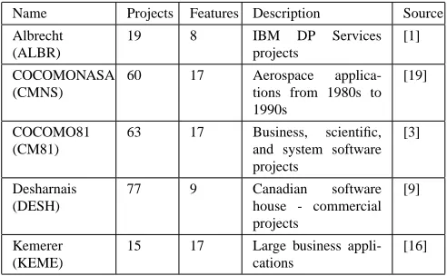
Name Projects Features Description Source
Albrecht (ALBR)
19 8 IBM DP Services
projects
[1]
COCOMONASA (CMNS)
60 17 Aerospace applica-tions from 1980s to 1990s
[19]
COCOMO81 (CM81)
63 17 Business, scientific, and system software projects
[3]
Desharnais (DESH)
77 9 Canadian software house - commercial projects
[9]
Kemerer (KEME)
15 17 Large business appli-cations
[16]
Table 1. Data sets used in the experiments
4. Experimental Method
4.1
Data Sources
Different researchers usually use different data sets to test their methods which makes it hard to compare their results. In order to compare our results with other researchers’ re-sults, and allow other researchers to confirm our rere-sults, we used five publicly available data sets as our data source. Most of these data sets have been used by more than one researcher to evaluate software cost estimation models. For example, COCOMO81 is the data set that was used by Boehm [3] to build the COCOMO model and also was used by Briand et al. [4], Srinivasan and Fisher [25], and Samson et al. [23] to compare different effort prediction methods; the Kemerer data set was coded by Kemerer [16] using the same attributes as Boehm and later was used by Briand et al. [4], Srinivasan and Fisher [25], and Shepperd and Schofield [24]; the Albrecht data set actually is the IBM DP Services data but was first used by Albrecht and Gaffney [1] and was also used by Shepperd and Schofield [24] to validate soft-ware size and effort estimation methods.
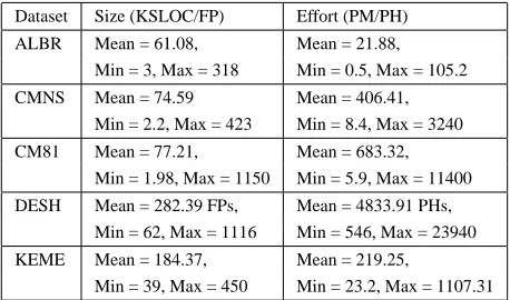
Tables 1 and 2 summarize these data sets and show that application domains range from business, science, and tech-nology to system software. The project size ranges from 1.98 KSLOC to 1150 KSLOC (or from 62 FPs to 1116 FPs), the project effort ranges from 0.5 person months to 11400 person months (or from 546 person hours to 23940 person hours), and the number of projects ranges from 15 to 77. Therefore, the data sets are quite diverse.
4.2
Validation method
Dataset Size (KSLOC/FP) Effort (PM/PH)
ALBR Mean = 61.08, Mean = 21.88, Min = 3, Max = 318 Min = 0.5, Max = 105.2
CMNS Mean = 74.59 Mean = 406.41, Min = 2.2, Max = 423 Min = 8.4, Max = 3240 CM81 Mean = 77.21, Mean = 683.32,
Min = 1.98, Max = 1150 Min = 5.9, Max = 11400
DESH Mean = 282.39 FPs, Mean = 4833.91 PHs, Min = 62, Max = 1116 Min = 546, Max = 23940 KEME Mean = 184.37, Mean = 219.25,
Min = 39, Max = 450 Min = 23.2, Max = 1107.31
Table 2. Descriptive statistics for project size and effort
and cover all projects, we used the jack knife methodology to validate the proposed GRACE method. Specifically, for each of thenprojects of a given data set, we predicted its effort with (k, ζ) which were learned from the remaining
n−1projects. The evaluation measures defined in subsec-tion 4.3 are then computed over thenpredictions.
For the purpose of evaluating the performance of the pro-posed GRACE method, we compared it with the stepwise regression method. For stepwise regression, the prediction models were generated using the entire data set. This means the results are likely to be slightly biased in favour of the re-gression models. In addition, we also compared our results with ANNs, linear regression, CARTX, and Analogy where the accuracy indicators and evaluation procedures permit.
4.3
Evaluation Criteria
We used the Bias, which refers to how far the average statis-tic lies from the parameter it is estimating, to assess the error which arises when estimating software effort. It is defined as follows:
Biasi=
Ei−Eˆi
Ei
×100 (8)
whereEˆiis the prediction of effortEi.
A common criterion for evaluating software effort pre-diction methods is the Magnitude of Relative Error (MRE). For a projectiwhose effort is predicted, the corresponding MREiis defined as follows:
MREi=|Biasi|, (9)
By averaging MREi over multiple projectsn, Mean MRE
(MMRE) is obtained:
MMRE= 1
n i=n
X
i=1
MREi. (10)
As MMRE is sensitive to individual predictions with exces-sively large MREs, we also use the median of MREs for thenprojects (MdMRE), which is less sensitive to extreme values, as another measure. For both MMRE and MdMRE, a higher score means worse prediction accuracy.
When using MRE as a measure of prediction accuracy, we suppose the error is proportional to the size of the project. Thus, PRED(l) is usually used as a complementary criterion. This is defined as follows:
PRED(l)= k
n×100 (11)
wherekis the number of projects where MREi ≤l%, and nis the number of all predictions. Unlike both MMRE and MdMRE, for PRED(l), a higher score implies better predic-tion accuracy.
5. Experimental Results
Tables 3 and 4 contain the accuracy of respective methods in terms of MMRE, MdMRE, PRED(25), and Bias. From Ta-ble 3 we observe that the MMREs and MdMREs of GRACE are much smaller than those of SWR except for the Deshar-nais data set. Here the two methods obtained almost the same MMRE and the SWR’s MdMRE is slightly better. Ex-cluding the Desharnais data set, MMREs have been reduced by at least 67.95% and MdMREs have been reduced by at least 21.36%. This suggests that GRACE tends to allow more accurate predictions than SWR.
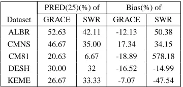
From Table 4 we observe that PRED(25) values are more mixed. GRACE has better values for 3 out of 5 data sets though this may in part be due to the arbitrary effect of set-ting the theshold to 25%. We also observe that the biases of GRACE for all data sets are no more than 19%, and are much smaller than those of SWR excepting the Desharnais data set. In 4 out of 5 data sets, GRACE over estimated effort. This means there may be scope for improving accu-racy.
At the same time, the use of the same data sets and the same experimental method — the jack knife — allow us to compare GRACE with Analogy [24], ANN [23], lin-ear regression [23], and CARTX [25]. Table 5 contains the published results. The results show that compared with Analogy, the MMRE and PRED(25)3 have been improved
by GRACE by 2.82% and 37.3% respectively with the Al-brecht data set, by 22.14% and -16.67% respectively with the Desharnais data set, and by 5.11% and -33.33% re-spectively with the Kemerer data set. The results show that compared with ANN, linear regression, and CARTX, the MMRE 4 has been improved by GRACE by 82.23%,
MMRE(%) of MdMRE(%) of Dataset GRACE SWR GRACE SWR
ALBR 60.25 103.02 21.35 45.02 CMNS 32.88 102.59 28.38 49.98 CM81 76.09 1540.84 60.52 445.13 DESH 49.83 49.63 33.93 30.94 KEME 58.83 102.61 46.94 59.69
Table 3. MMRE and MdMRE of GRACE and SWR with different data sets
PRED(25)(%) of Bias(%) of Dataset GRACE SWR GRACE SWR
ALBR 52.63 42.11 -12.13 50.38 CMNS 46.67 35.00 17.34 34.15 CM81 20.63 6.67 -18.89 578.18 DESH 30.00 32 -16.52 -14.99 KEME 26.67 33.33 -7.07 -47.54
Table 4. PRED(25) and Bias of GRACE and SWR with different data sets
85.39%, and 39.23% respectively with the COCOMO81 data set.
We are also aware that Burgess and Lefley [7] using a Genetic Programming approach obtained a better result of MMRE=44.5% for the Desharnais data set. Unfortunately, a different experimental method — holdout — was used, and the model was tested on only 22% projects. The test data set is small, as it is common to designate 1/3 of the data as the test set. Therefore, it is not directly comparable. Generally, it is not recommended to compare methods with the same data sets but with different experimental methods. For example, Mair et al.[18] report a 57% of MMRE with the Analogy method with the Desharnais data set. Unfor-tunately, for the same data set, Shepperd and Schofield’s [24] result is 64%. The reason is the former used a hold-out method, whereas the experimental method used by the latter is the jack knife. Another example is both Srinivasan and Fisher [25] and Briand et al.[4] used the regression and decision trees method and the same data sets. More impor-tantly they used the same experimental method – holdout, but different training sets and test sets. Unfortunately, they obtained very different results. Srinivasan and Fisher’s re-sult is 364% in terms of MMRE and Briand et al. obtained a 94% of MMRE.
To summarize, in 4 out of 5 data sets, GRACE is more accurate than SWR and almost as good as SWR for another data set; in all the comparable cases, GRACE tends to be more accurate than the other compared methods at least for the given data sets.
Dataset MMRE (%) of
ALBR GRACE 60.25 Analogy 62
CM81 GRACE 76.09 ANN 428.11 Lin.RegR. 520.71 CARTX 125.2 DESH GRACE 49.83 Analogy 64
KEME GRACE 58.83 Analogy 62
Table 5. Comparison with published results with the same dataset and the same experi-mental method
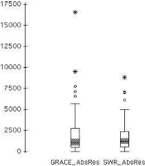
The boxplot is a type of graph that is used to show the shape of the distribution, its central value, and variability. We used boxplots to explore the spreads of absolute resid-uals of prediction accuracy for GRACE and SWR methods with all five data sets.
Figs. 1, 2, 3, 4, and 5 are the boxplots of absolute residu-als of prediction accuracy for GRACE and SWR with the Albrecht, COCOMONASA, COCOMO81, Kemerer, and Desharnais data sets respectively.
From Fig. 1 we observe that: 1) the smaller box of SWR indicates reduced variability of absolute residuals; 2) the median of GRACE is far smaller than that of SWR. This means that at least half of the predictions of GRACE are more accurate than those of SWR.
From Fig. 2 we observe that: 1) the range of absolute residuals of GRACE excluding outliers is smaller than that of for SWR, which means smaller variance; 2) the box of GRACE overlays the lower whisker. This reveals that the data are probably skewed towards the lower end of the scale, and also shows more accurate results; 3) the smaller box of GRACE indicates reduced variability of absolute residuals; 4) the median of GRACE is smaller than that of SWR.
From Fig. 35 we observe that: 1) the range of
abso-lute residuals of GRACE excluding outliers is much smaller than that of SWR, which means smaller variance; 2) the box of GRACE overlays the lower whisker. This reveals that the data are probably skewed towards the lower end of the scale, and also means more accurate results; 3) the smaller box of GRACE indicates reduced variability of absolute residuals; 4) the median of GRACE is much smaller than that of SWR. From Fig. 4 we observe that 1) the range of abso-lute residuals of GRACE excluding outliers is somewhat smaller than that of SWR, which means smaller variance; 2) the smaller box of GRACE indicates reduced variability
5The scale has been truncated so the even worse outliers for SWR are
Figure 1. Absolute residuals of prediction ac-curacy for GRACE and SWR with the Albrecht data set
of absolute residuals; 3) yet again the median of GRACE is smaller than that of SWR.
From Fig. 5 we observe that 1) similar sized boxes mean-ing similar variability of the non-outlier absolute residuals; 2) almost the same median means that at least half of the predictions are at the same accurate level; 3) there are more extreme outliers for the GRACE method.
Figs. 1 - 5 are all characterized by a few extreme outliers, but more so for GRACE. After investigating the data sets, we found that these outliers are related to the noise in the corresponding data sets. The reason why GRACE is more sensitive to noise is that SWR uses all the projects’ data. That is, it uses the models learned from projects to predict themselves; but GRACE usesn−1projects to predict the unseen project. Therefore, if a ‘new’ project itself is noise, the corresponding result is an outlier as well. Of course, any machine learning method can suffer from “garbage in garbage out (GIGO)” and we cannot learn useful knowledge from garbage. It may also be useful in the future to explore when a prediction cannot sensibly be made.
Thus, quality data is a precondition for obtaining quality knowledge, and data quality is a constant issue for machine learning and data mining researchers. This reminds us that before predicting software effort, we should firstly remove outliers. Alternatively one might consider dividing highly distinct projects into separate data sets.
To summarize, the boxplots of absolute residuals of pre-diction accuracy for GRACE and SWR with five data sets show GRACE outperformed SWR.
6. Conclusions and Future Work
In this paper, we have proposed a novel approach of using Grey Relational Analysis of Grey System Theory to address feature subset selection and software effort prediction at an early stage of a software development process.
Figure 2. Absolute residuals of prediction ac-curacy for GRACE and SWR with the CO-COMONASA data set
Figure 3. Absolute residuals of prediction ac-curacy for GRACE and SWR with the CO-COMO81 data set
Figure 5. Absolute residuals of prediction ac-curacy for GRACE and SWR with the Deshar-nais data set
Using five publicly available data sets, we have com-pared the proposed method with prediction models based on stepwise regression, and when available, also with Anal-ogy, artificial neural networks, linear regression, and regres-sion and deciregres-sion trees. The results show that the proposed method outperformed other methods in terms of MMRE, MdMRE, PRED(25) and Bias for the majority (4 out of 5) of data sets we used. This is very encouraging and indicates that the method has considerable potential.
However, this work is just a first step in using GST to systematically address software effort prediction questions. Therefore, future work, apart from improving our GRACE method, includes developing a GST-based missing data im-putation method. This is because many software project data sets contain missing data, and all the project data are incomplete in the early stages of development processes. At the same time, almost all the project prediction methods re-quire complete data sets. Therefore, to use these methods we must firstly make data sets complete either through miss-ing data ignormiss-ing techniques or through missmiss-ing data impu-tation techniques. However, the former techniques make small software project data sets more smaller, and further hinder effort prediction. GST is therefore proposed for pro-cessing small data sets since by measuring the relationship between data series, we can find the appropriate values for missing data.
It may also be fruitful to develop a GST based project effort continuous prediction method. Remember that soft-ware processes take place over time. This calls for contin-uous effort prediction. Taking these factors into account, our effort prediction method will be based on GST that will dynamically predict project effort at different time-points during software projects capitalising upon updated or new information.
Thus overall, we are of the opinion that using Grey Sys-tem Theory for software project effort prediction should be
further explored. We have demonstrated accuracy levels that are broadly comparable or better than regression mod-els or other machine learners. We have also argued that there is more of the theory that can be usefully exploited to deal with missing data values and to support ongoing as opposed to one-shot prediction. However, independent val-idation of these ideas is essential before it will start to be possible to generalize from our results to other data sets.
Acknowledgments
This work was funded by the UK Engineering and Physical Sciences Research Council under grant GR/S45119. The authors would like to thank the three anonymous reviews for their insightful and helpful comments.
References
[1] Albrecht, A. and Gaffney, J. “Software Function, Source Lines of Code, and Development Effort Pre-diction”. IEEE Transactions on Software Engineering, Vol.9, No.6, pp639–648, 1983.
[2] Boehm, B.W., “Software Engineering Economics”.
IEEE Transactions on Software Engineering, Vol.10,
No.1, pp4–21, 1984.
[3] Boehm, B.W., Software Engineering Economics, Prentice-Hall, 1981.
[4] Briand, L., Basili, V., and Thomas, W., “A Pattern Recognition Approach for Software Engineering Data Analysis”. IEEE Transactions on Software
Engineer-ing, Vol.18, No.11, pp931–942, 1992.
[5] Briand, L., T. Langley and I. Wieczorek. “Using the European Space Agency data set: a replicated assess-ment and comparison of common software cost mod-eling techniques”. 22ndInternational Conference on
Software Engineering, pp377–386, Limerick, Ireland:
Computer Society Press, 2000.
[6] Briand, L.C. and Wieczorek, I.,“Resource Modeling in Software Engineering,” in Encyclopaedia of
Soft-ware Engineering, J. J. Marciniak, Ed., 2nd ed. New
York: John Wiley, 2002.
[7] Burgess, C.J. and Lefley, M., “Can genetic program-ming improve software effort estimation? A compar-ative evaluation”. Information and Software
Technol-ogy, Vol.43, No.14, pp813–920, 2001.
[8] Deng, J. L., “Control problems of grey system”.
[9] Desharnais, J. M., “Analyse statistique de la produc-tivitie des projets informatique a partie de la technique des point des fonction”. Masters Thesis, University of Montreal, 1989.
[10] Finnie, G.R and Witting, G.E., “A comparison of software effort technique: using function points with neural networks, case based reasoning and regres-sion models”. Journal Systems and Software, vol.39, pp281–289, 1997.
[11] Huang, S. J., Huang, C. L., “Control of an inverted pendulum using grey prediction model”. IEEE
Trans-actions on Industry Applications, vol.36, no.2, pp452–
458, 2000.
[12] Jain, A. and Zongker, D., “Feature Selection: Eval-uation, application and small sample performance”.
IEEE Transactions on Pattern Analysis and Machine Intelligence, vol.19, no.2, pp153–158, 1997.
[13] Jiang, B.C., Tasi, S. L., and Wang, C. C., “Ma-chine vision-based gray relational theory applied to IC marking inspection”. IEEE Transactions on
Semi-conductor Manufacturing, vol.15, no.4, pp531–539,
2002.
[14] Jørgensen, M., Indahl, U., and Sjøberg, D.,“Software effort estimation by analogy and ‘regression toward the mean’ ”. Journal of Systems and Software, Vol.68, No.3, pp253–262, 2003.
[15] Jou, J. M., Chen, P. Y., and Sun, J. M., “The gray pre-diction search algorithm for block motion estimation”.
IEEE Transactions on Circuits and Systems for Video Technology, vol.9, no.6, pp843–848, 1999.
[16] Kemerer, C.F., “An empirical validation of software cost estimation models”. Comm. ACM, vol.30, no.5, pp416–429,1987.
[17] Luo, R. C., Chen, T. M., and Su, K. L., “Target track-ing ustrack-ing a hierarchical grey-fuzzy motion decision-making method”. IEEE Transactions on Systems, Man
and Cybernetics, Part A, vol.31, no.3, pp179–186,
2001.
[18] Mair, C., Kadoda, G., Lefley, M., Phalp, K., Schofield, C., Shepperd, M. and Webster, S., “An investigation of machine learning based prediction systems”.
Jour-nal of Systems and Software. Vol.53, No.1, pp23–29,
2000.
[19] Menzies, T., Port, D., Chen, Z., Hihn, J. and Stukes, S., ”Validation Methods for Calibrating Software Ef-fort Models”. The 27th International Conference on
Software Engineering. St Louis Missouri, USA, 15–
21 May, 2005.
[20] Moløkken, K. and Jørgensen, M., “A review of sur-veys on software effort estimation”, 2nd Intl. Symp.
on Empirical Software Engineering, pp223-230: IEEE
Computer Society, 2003.
[21] Mukhopadhyay, T., Vicinanza, S.S., and Prietula, M.j. “Examining the feasibility of a case-based reasoning model for software effort estimation.” MIS Quarterly, vol.16, pp155–171, june, 1992.
[22] Putnam, L. H., “A general empirical solution to the macro software sizing and estimation problem”. IEEE
Transactions on Software Engineering, vol.4, no.4,
pp345–381,1978.
[23] Samson, B., Ellison, D., and Dugard, P., “Software coast estimation using an Albus Perceptron (CMAC)”.
Information and Software Technology, vol.39, nos.1/2,
1997.
[24] Shepperd M. and Schofield C., “Estimating Software Project Effort Using Analogies”. IEEE Transactions
on Software Engineering, Vol.23, No.12, pp736–743,
1997.
[25] Srinivasan, K. and Fisher, D., “Machine Learning Approaches to Estimating Software Development Ef-fort”. IEEE Transactions on Software Engineering, Vol.21, No.2, pp126-137, 1995.
[26] Su, S. L., Su, Y. C., Huang, J. F., “Grey-based power control for DS-CDMA cellular mobile sys-tems”. IEEE Transactions on Vehicular Technology, vol.49, no.6, pp2081–2088, 2000.
[27] Wang, Y. F. “On-demand forecasting of stock prices using a real-time predictor”. IEEE Transactions on
Knowledge and Data Engineering, vol.15, no.4,
pp1033–1037, 2003.
[28] Witting, G.E. and Finnie, G.R, “Using artificial neu-ral networks and function points to estimate 4GL soft-ware development effort”. Australian Journal of
Infor-mation Systems,vol.1, no.2, pp87-94, 1994.
[29] Wu, J.H. and Chen C. B., “An alternative form for Grey Relational Grade”. Journal of Grey System, vol.11, no.1, pp7–11,1999.
[30] Wu, H. S., Deng, J. L., and Win, K. L., Introduction
to Grey Theory (in Chinese). Taipei, Taiwan: Gao-Li